Modelling Extreme Tail Risk of Bitcoin Returns Using the Generalised Pareto Distribution

Abstract

This paper analyses the extreme tail behaviour of Bitcoin returns by fitting a Generalised Pareto Distribution (GPD). The GPD is used to model the extreme daily Bitcoin returns over the period 2008 to 2023. The returns above the chosen thresholds, for both Bitcoin gains and losses, are selected. The GPD is then fitted to the selected excess returns. The Anderson Darling (AD) and Kolmogorov Smirnov (K-S) goodness-of-fit tests reveal that the GPD captures the distribution of the Bitcoin excess returns. The Value at Risk (VaR) and Expected Shortfall (ES) under the GPD are used to measure the extreme tail risk of the Bitcoin returns. The upside risk (gains) is found to outweigh downside risk (losses), and this gives insight to investors interested in Bitcoin.

1. Introduction

Predicting the likelihood of an extreme event within a given period is often reflected in the volatility of that event. Statistical methods have proved effective in forecasting extreme movements of financial events, and in this case, focus is given to Bitcoin extreme price index movements. A Generalised Pareto Distribution (GPD) is a family of continuous probability distributions which falls under extreme value theory (EVT) [1]. Ever since the EVT was developed in the 1920s, it has been used to predict the occurrence of several different extreme events including financial market crashes and other black swan events [2, 3]. EVT has been applied to the crypto currency market to predict cryptocurrency price movements using the Generalised Extreme Value distribution [4]. The aim of this paper is to show how the EVT based GPD models extreme Bitcoin gains and losses and assessing the risk levels thereof.

2. Review of literature

Bitcoin, for several years, has had the largest market share in the crypto industry. Evidence in the literature suggests that much research has been done on Bitcoin [5, 6, 7, 8, 9]. Research done by Osterrieder and Lorenz [10] showed Bitcoin extreme price changes to be violating the usual normal distribution assumption. The selection of an appropriate statistical distribution to asset returns becomes the challenge. Osterrieder and Lorenz [10] conducted a study on the extreme tail behaviour of Bitcoin where he performed an in-depth extreme univariate analysis. Bitcoin was found to exhibit volatility that was higher than the Group of 10 (G10) countries’ currencies. The G10 countries comprise of Belgium, Canada, France, Germany, Italy, Japan, the Netherlands, Sweden, Switzerland, the United Kingdom and the United States. Non-normality and heavier tails were observed to be stronger in Bitcoin prices, in comparison to the G10 countries’ currencies. In extreme value analysis, there are two approaches to selecting extremes, and these are the block maxima and the peaks-over threshold methods [11]. Islam and Pial Das [7] conducted a study on predicting Bitcoin returns using Extreme Value Theory (EVT). Extreme Bitcoin returns were modelled using the block maxima and the peak over threshold approaches. It was concluded that Bitcoin extreme tail distributions are well represented by the EVT based distributions and that investors can make use of the results of their findings. The authors used return levels as measures of risk. This paper uses the Basel III recommended Value at Risk (VaR) to quantify risk. VaR is used in quantifying minimum capital requirements. The Expected Shortfall (ES) is also used in this paper to quantify extreme risk in Bitcoin on this updated dataset. Moreover, this paper separates gains from losses in the analysis.

Cryptocurrencies are considered highly volatile and show extreme tail movements when compared to traditional financial markets and fiat currencies [12, 13]. In this study, research is conducted on the Bitcoin extreme gains and losses by fitting the GPD. Risk analysis measures, such as VaR and ES are computed on the Bitcoin extreme returns. The peaks over threshold based GPD is chosen over the block maxima based Generalised Extreme Value Distribution (GEVD) as the former makes use of the data more efficiently.

This research extends EVT applications by fitting the GPD and in quantifying the extreme volatile behaviour of Bitcoin log returns using the VaR and the ES as measures of risk.

3. Methodology

This section describes the methods and tools that are used in the study. The properties of empirical distribution used in the analysis of the returns are also explained. Descriptions of the criteria that are used in the data selection process and in the goodness of fit tests on the extreme tails of the Bitcoin returns are explained as well. The GPD is applied on the Bitcoin extreme price returns data in order to analyse the tail behaviour of Bitcoin extreme returns. The threshold selection methods to be applied to the Bitcoin returns data are also discussed. The returns are defined as:

$$z_t=log\left(\frac{P_t}{P_{t-1}}\right)=log\left(P_t\right)-log\left(P_{t-1}\right),$$E1

where $P_t$ represents the price of Bitcoin at time $t$ and $P_{t-1}$ represents the price at time $t-1$.

3.1 Data selection process

The data used in the study are taken from CoinMarketCap “Cryptocurrency Market Capitalizations” and retrieved from https://coinmarketcap.com/ on September 01 of 2023. The data is of the period 28 April 2013 to 1 September 2023. There are four data sets for Bitcoin prices considered, which are the daily opening prices, daily closing prices, daily low and daily high prices. The Bitcoin daily closing price data were finally chosen for carrying out the analysis. Any of the 4 data sets could have been used since they all had similar descriptive statistics features. The Bitcoin daily closing prices used in this study are an average of the closing price values from several Bitcoin exchanges.

3.2 Extreme value theory (EVT) – peak over threshold

The peaks-over-threshold (PoT) analysis, also known as the partial durations series analysis in some more applied fields, has played a fundamental role in the development of statistical EVT. It is based on fitting a GPD to the data exceedances above a large enough threshold.

3.3 Generalised Pareto distribution (GPD)

The GPD emerges from the EVT. It models values of a given random variable that are above a certain threshold value. Threshold simply means a point on a statistical distribution above which values can be taken as extreme. The data used for a GPD can be ordered from the smallest observed excess to the highest observed excess. The excess of the values observed above the threshold is also known as the exceedances and are peaks over a threshold. For instance, if there is an ordered set of values of a random variable such that $\mathrm{Z}$ is $z_1,z_2,z_3,\dots ,z_{n-1},z_n.$, where $z_n$ is the largest of the values of $Z$, then the peaks over threshold or excesses/exceedances are denoted as $x_i=z_i-\mu$.

The data of the exceedances is known to follow the GPD and with a probability density function of the form:

$$f\left(z_i;\beta ,\gamma \right)=\left\{\begin{array}{c}\frac{1}{\beta }\left(1+\gamma {\left(\frac{z_i-\mu }{\beta }\right)}^{-\frac{1}{\gamma }-1}\right)\text{for}\gamma \ne 0\\ \frac{1}{\beta }exp\left(\frac{\mu -z_i}{\beta }\right)\text{for}\gamma =0\\ ,\end{array}\right.$$E2

where $\mu$ is the threshold value,$\beta$ is the scale parameter and $\gamma$ is the shape parameter.

From Eq. (2) a corresponding Cumulative Distribution Function (CDF) for the GPD is derived and is given as:

$$F\left(z_i;\beta ,\gamma \right)=\left\{\begin{array}{c}1-{\left(1+\frac{\gamma \left(z_i-\mu \right)}{\beta }\right)}^{-\frac{1}{\gamma }}\text{for}z\in \left[u,\infty \right]\text{and}\gamma \ne 0\\ 1-exp\left(-\frac{\left(z_i-\mu \right)}{\beta }\right)\text{for}z\in \left[u,\infty \right]\text{and}\gamma =0\end{array}\right.$$E3

From Eq. (3), if z follows the GPD ($\gamma ,\beta$), then$z+\mu$ is a GPD ($\gamma ,\beta +\mathit{\mu \gamma }$), given that $z>\mu$ for any threshold value$\mu$. It also implies that$z-\mu$, provided$z>\mu$, follows a GPD ($\gamma ,\beta -\mathit{\mu \gamma }$). Castillo and Hadi [14] stipulated that consistence of a model with a data set goes hand in hand with the model being consistent with the same data set for all high threshold values. Another interesting fact about the GPD is that, for a certain range of values for$\gamma$, the GPD reduces to certain types of common distributions.

The following cases show a resulting distribution from a GPD when the parameter $\gamma$ takes certain values:

1. Case 1: when$\gamma =0$, the GPD reduces to a two-parameter exponential distribution with a mean denoted by$\beta$. This distribution is often described as light tailed.

2. Case 2: when$\gamma \le -0.5$, its variance is equal to$\infty$, meaning that if$\gamma >-\frac{1}{n}$, and then the nth central moment exists.

3. Case 3: if$\gamma <0$, the GPD becomes a Pareto type II distribution which has a bounded tail.

4. Case 4: when$\gamma =1$, the GPD reduces to a uniform distribution U [0,$\beta$].

5. Case 5: when$\gamma >0$, the GPD becomes an ordinary heavy tailed Pareto distribution.

3.4 Threshold selection for the GPD

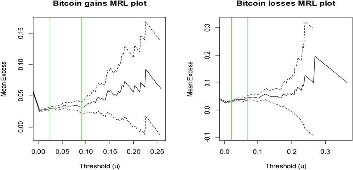
Adopting a low threshold value results in sensible approximations to the peaks-over threshold for the GPD with a relatively large sample size [15]. Lower threshold values give an advantage of credibility especially in cases where the main body of data is not sufficient for analysis. However, the theory of convergence to the GPD may not hold and often results in bias in such cases. Too large of a threshold result in fewer observations with a high variance in parameter estimation. The high variance is a result of having fewer extreme values caused by a selection of this very high threshold. Hence a good threshold value is chosen such that a balance should be achieved between variance and bias. There are several threshold selection methods but only three are used in this study, and these are the Pareto Q-Q plot, the mean excess plot and the parameter stability plot. Graphs in Figure 1 show the peaks-over thresholds selection methods for the Bitcoin gains and losses data respectively. Losses are negative returns turned to positive values by multiplying with a negative one. This is done for easier analysis and distribution fitting.

Figure 1.

Mean residual live plot of bitcoin positive and negative returns.

3.5 Mean excess plots

The main idea behind the mean excess plots is to find the extent to which an observed value $z$ exceeds a certain extrema threshold value given that the observed value is greater than the threshold value$,\mu$. In mathematical terms, the mean excess equation is denoted as:

$$e\left(\mu \right)=E\left(Z-\mu |Z>\mu \right).$$E4

For a set of independent extreme events, the mean excess is defined as the mean of all the values above the threshold, provided the values are arranged in order such that the last is the maximum. If $z_1,z_2,z_3,\dots ,z_{n-1},z_n$ are the values of the variable Z arranged in order, then $z_n$ would be the maximum. This method is carried out at 95% confidence level such that the expected threshold value is found to be lying in the expected confidence interval. Observing a straight positive gradient from bottom left to top right depicts a fat tailed GPD that has a positive shape parameter. If the gradient of the slope is negative, then the mean excess plot depicts or indicates a thin-tailed behaviour. The mean residual plots for the Bitcoin gains and losses are shown Figure 1.

Based on the two graphs in Figure 1, the threshold is favourably stable between 0.02 and 0.08 for both the Bitcoin gains returns and the Bitcoin losses as shown by the green lines on the graphs above, therefore the threshold value is most likely to be between the values 0.02 and 0.08.

3.6 Pareto Q-Q plot

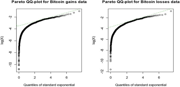
The Pareto Q-Q plot method pinpoints the threshold and involves fitting a regression line to the data points in the Pareto Q-Q plot. It is possible to check whether a model is plausible enough to be a good fit for the data. The Q-Q plots are easy to compute, especially for the exponential distribution [16]. The point where the fitted tangent regression line cuts the y-axis (z-axis in this instance) is used to calculate the threshold value in the data set. The exponent of the value where the regression line cuts through the y-axis (z-axis) is taken as the threshold value. The green dotted line in the two graphs in Figure 2 shows the regression line.

Figure 2.

Q-Q plots for bitcoin positive and negative log returns.

The threshold values for the Bitcoin gains and for the Bitcoin losses are observed to be approximately equal to the exponent of −3.5 and −3.7 respectively, corresponding to 0.03 and 0.025 respectively. The Q-Q plots for the Bitcoin price returns for gains and losses are shown in Figure 2.

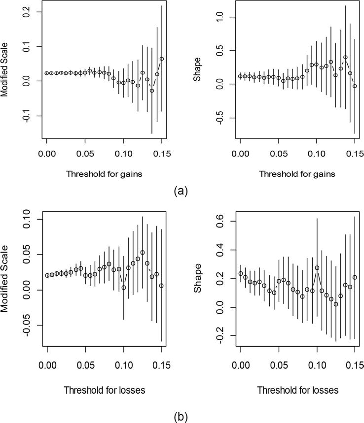
Based on Figure 2, threshold values of 0.03 and 0.025 are selected for gains and losses respectively (after rounding to three decimal places), and 578 and 613 exceedances are obtained for gains and losses respectively. The parameter stability plots for gains are in Figure 3a.

Figure 3.

(a) Parameter stability plots for gains. (b) Parameter stability plots for losses.

The parameter stability estimate plots in Figure 3a and b, support the reasonable and suggested thresholds from the pareto Q-Q plots of 0.0302 and 0.0247 for Bitcoin gains and losses respectively, since stability is observed at around these threshold values. The same can be said of the results from the mean residual live plots.

3.7 Risk measures

Risk measures used in this study are the VaR and ES.

3.8 Value at risk (VaR)

The VaR refers to the maximum amount of potential loss on a security or a portfolio over a period, with a given degree of confidence. In other words, it generalises the probability of underperforming by providing a statistical measure of downside risk. VaR can be in two forms, depending on the state of the data or distribution being considered. We will only look at the continuous case since the distribution of Bitcoin gains and losses data is continuous in nature. For a continuous random variable Z, VaR is defined as:

$$\mathrm{VaR}\left(\mathrm{Z}\right)=-t\text{where}P\left(Z<t\right)=p.$$E5

VaR is measured based on assumptions that may not be apparent on immediate terms. In most practical terms, normality is assumed. It is known that securities or portfolios exposed to systematic bias, credit risk or derivatives may not exhibit normality [17]. In such circumstances, the usefulness of VaR would depend on modelling the skewness of the returns data in the form of the GPD or via monte carlo simulations. The fatter the tail, the more lacking the data is in the very extremities.

3.9 VaR in extreme value using GPD

The VaR for the GPD is computed as:

$$\widehat{\mathit{V}\mathit{a}\mathit{R}}=\left\{\begin{array}{c}\mu +\frac{\widehat{\beta }}{\widehat{\gamma }}\left\{{\left(\frac{n}{N_{\mu }}p\right)}^{-\gamma }-1\right\}\widehat{\gamma }\ne 0\\ \mu -\widehat{\beta }log\left(\frac{n}{N_{\mu }}\left(1-p\right)\right)\widehat{\gamma }=0\end{array}\right.$$E6

where the period length is denoted by $n$, with $\mathrm{\beta }\text{and}\gamma$ being the scale and shape parameters respectively, of $n$ returns in a period [17]. The maximum likelihood estimate (MLE) is used to estimate the parameters as it results in unbiased, more efficient, and minimum variance estimators. The variable $p$ denotes the probability of the small upper tail.

3.10 Expected shortfall (ES)

The ES is the average of all the returns in a distribution that are worse than VaR of the portfolio at a given level of confidence. For example, for a 95% confidence level, ES is obtained by taking the average of returns in the worst 5% of cases. It provides a return expected that exceed VaR for a given level of probability. In a general continuous case, the ES is given as:

$$\mathrm{ES}=E\left[max\left(L-Z,0\right)\right]={\int }_{-\infty }^L\left(L-Z\right)f\left(z\right)\mathit{dz},$$E7

where $L$ is the chosen benchmark level. In a general discrete case, the ES is given by:

$$\mathrm{ES}=E\left[\mathit{max}\left(L-Z,0\right)\right]={\sum }_{z<L}\left(L-z\right)P\left(Z=z\right).$$E8

In extreme value for the GPD, ES = $\mathit{Va}{R}_p+E(Z-\mathit{Va}{R}_p\mid Z>\mathit{Va}{R}_p$), where $\mathit{Va}{R}_p$ represents the threshold given value.

4. Results and discussion

The calculated thresholds are used to find the exceedances/excesses in fitting the GPD to the losses and gains.

4.1 GPD for the bitcoin losses data

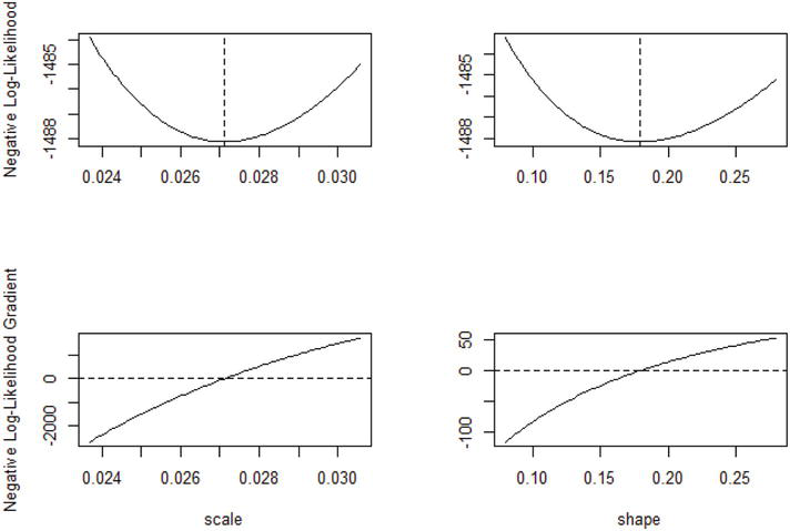
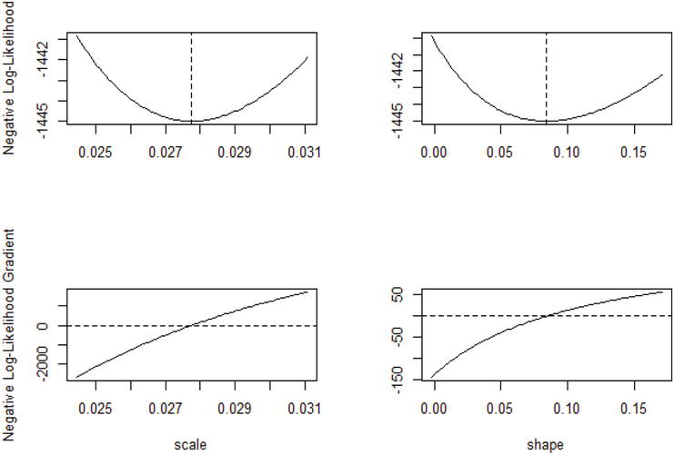
The Bitcoin losses which are above the chosen threshold of 0.025 are used in the analysis using the GPD. The GPD is fitted, and the parameter estimates are found through the MLE approach. This threshold value is obtained from the Q-Q plot and other threshold selection methods used in the previous section. The maximum likelihood estimates for both the shape parameter $\gamma$ and scale parameter $\beta$ are observed to be approximately 0.1796 and 0.0271 respectively. Since the confidence interval of the shape parameter $\gamma$ is greater than 0 at the 95% level of significance, it means that the GPD reduces to a type two Pareto distribution. Thus, a heavy tailed Pareto type two distribution can be used to model the Bitcoin losses. However, we begin by finding if the Bitcoin data can be modelled by the GPD. Figure 4 shows the likelihood function of both the scale and shape parameters.

Figure 4.

Maximum likelihood estimation of scale and shape parameters of losses under GPD.

It can be seen from Figure 4 that the shape parameter $\gamma$ has a value of 0.1796 with a calculated standard error of 0.0499, whereas the scale parameter $\beta$ has a value of 0.0271 with standard error 0.0017. The shape parameter is above $0$, and this means that tail losses are heavier than implied by the normal distribution tail. As a result, extreme losses may occur than anticipated if the data was normally distributed.

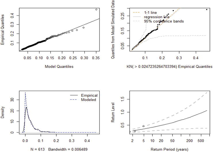
Figure 5 shows the model diagnostic plots for the GPD fit to the Bitcoin losses.

Figure 5.

Density and return plots for the GPD on bitcoin losses data.

The plots in Figure 5 show that the model is a good fit to the data since most of the data points are collinear and inclined at 45° to the horizontal on the Q-Q plot. The density plot also shows the same evidence as that provided by the Q-Q plot. Therefore, it is concluded that the GPD model is a good fit. A further analysis is done by testing the following hypotheses:

1. ${\mathrm{H}}_0:\text{The Bitcoin losses follow the}\mathrm{GPD}.$

2. ${\mathrm{H}}_{\mathrm{a}}:\text{The Bitcoin losses}\mathrm{do}\text{not follow the given}\mathrm{GPD}.$

The results of the tests, using maximum likelihood estimation, are given in Table 1.

GPD	AD statistic	AD p-value	K-S statistic	K-S p-value
Negative bitcoin returns	0.4871	0.76	0.0058	0.8895

Table 1.

Tests on goodness-of-fit of the GPD.

Table 1 results show that the Bitcoin losses follow a GPD since the p-values are large and hence there is not enough evidence to reject the null hypothesis.

4.2 GPD for the bitcoin gains data

The Bitcoin gains data over the chosen threshold of 0.03 are used to find out if the GPD can be a good fit to the data, and parameter estimates are found using the MLE approach. This threshold value is derived from evidence given by the Pareto Q-Q plot and other methods used. The log likelihood estimated values for both the shape parameter $\gamma$ and scale parameter $\beta$ are observed to be 0.0842 and 0.0278 respectively.

Figure 6 shows the likelihood functions for both the scale and shape parameters.

Figure 6.

Maximum likelihood functions for the scale and shape parameter on bitcoin gains data.

Figure 6 shows that the shape parameter $\gamma$ has a value of 0.0842 and the calculated standard error is 0.0433. The scale parameter is 0.0278 with standard error of 0.0017. Figure 7 shows model diagnostic plots for the GPD fit to the Bitcoin gains data above the threshold of 0.0302. The shape parameter is above 0, and this means that the left tail is heavier than the normal distribution tail. As result, extreme gains are more probable to occur.

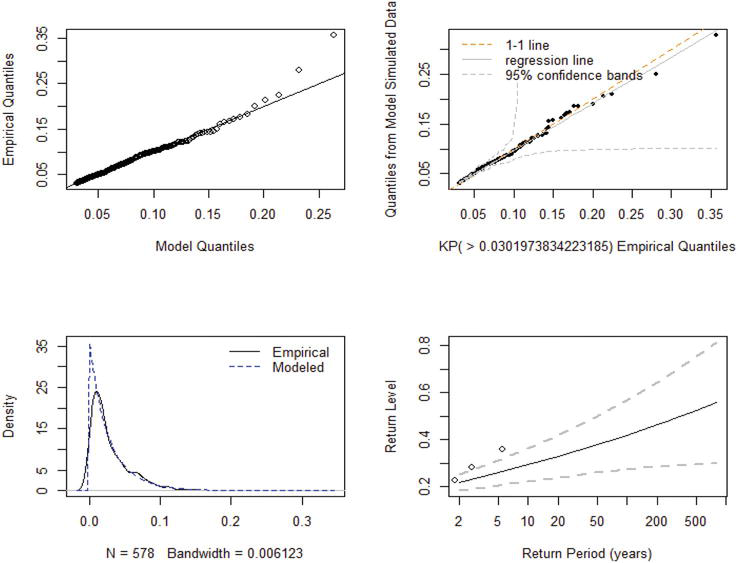
Figure 7.

Diagnostic plots for the GPD fit to the bitcoin gains data above the threshold of 0.03.

The plots in Figure 7 show that the model is a good fit to the data points using the GPD. From the Q-Q plot (top left), there is a strong indication of linearity for most of the data points. Moving from left to right, the largest quantiles divert from the 45° reference line with few values in the extreme top right. One can still say that the GPD is a good fit for the gains. The top right plot in Figure 7 shows the quantiles from a sample drawn from the fitted GPD against the empirical data quantiles with 95% confidence bands in dashed lines. Most of the quantiles (black dots) align with the 45°line dashed orange and fall in the confidence bands, which makes for a reasonable GPD fit.

The GPD density function (dashed blue) is overlaid on the empirical density in the bottom left plot and there are some similarities in kurtosis as is in the case for losses.

The return level plot is shown on the bottom right with 95% confidence intervals for the 5-year return level of the logarithm returns of monthly data. Therefore, it can be said at 95% confidence level, that the logarithmic returns will be above the range 0.2 to 0.3, at 95% confidence level.

However, we further investigate the goodness-of-fit of the GPD on Bitcoin gains data by carrying out a goodness of fit test on the following hypotheses:

1. $H_0:\text{The Bitcoin gains data follow the}\mathrm{GPD}.$

2. $H_a:\text{The Bitcoin gains data}\mathrm{do}\text{not follow the}\mathrm{GPD}.$

Table 2 gives the results of the test.

GPD	AD statistic	AD p-value	K-S statistic	K-S p-value
Gains	0.3730	0.8751	0.0055	0.9202

Table 2.

Tests on goodness-of-fit of the GPD on bitcoin gains data.

It is evident that Bitcoin gains data follow a GPD as shown by the AD and K-S statistics since the p values are greater than 0.05. It follows that an ordinary Pareto distribution can be a good fit since $\gamma$ is greater than 0 at 5% significance level. Two risk measures, VaR and ES, are applied to the data on gains and losses. The risk values obtained are shown in Tables 3 and 4.

Alpha (probability)	0.1	0.05	0.01
Gains	0.0581	0.0735	0.1060
Losses	0.0512	0.0628	0.0850

Table 3.

VaR results.

Alpha (Probability)	0.1	0.05	0.01
Gains	0.0792	0.0934	0.1233
Losses	0.0664	0.0763	0.0950

Table 4.

ES results.

4.3 Measures of risk from the GPD

Gains are riskier than losses as the gains are associated with higher values of VaR.

Gains are confirmed to riskier than losses in Table 4 as the gains are associated with higher values ES.

The GPD VaR and ES values at 99% confidence level are 0.1060 and 0.1233 for the gains, and 0.0850 and 0.0950 for the losses respectively. The interpretation of the upper tail risk values is that the expected gain in the Bitcoin market has a 99% likelihood that it will not exceed 0.1060 but if it does exceed, it will come to an average of 0.1233. The interpretation of the losses risk value is that the expected loss in the Bitcoin market has a 99% likelihood that it will not exceed 0.0850 but if it does exceed, it will come to an average of 0.0950. Analogously, the VaR and ES values, at different probability levels, are explained in the same way.

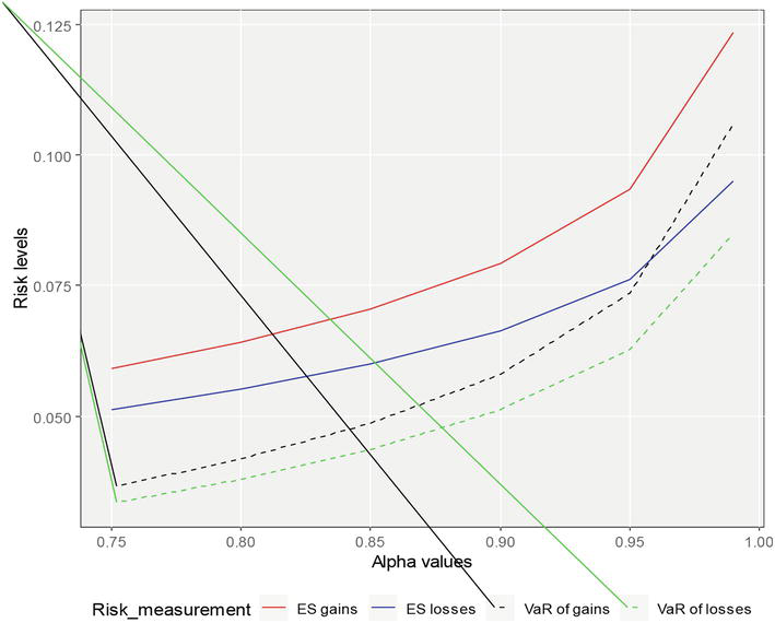
The Figure 8 shows the risk measurement values on Bitcoin market returns from 75% confidence level to as much as 99% confidence level. The risk values are plotted against the alpha probability values. It is clearly that the gains have a higher VaR and ES than the losses. In other words, gains seem to outweigh losses, and this can have a good implication to interested investors in Bitcoin, especially the risk seeking investors, in exploring the possibility of higher returns whilst minimising losses. At all alpha values, the VaR and ES of gains are greater than the corresponding values for losses. It is possible to net in those extreme gains. The losses would be smaller is they were to occur.

Figure 8.

GPD VaR and ES values to the bitcoin gains and losses returns data.

5. Conclusion

Bitcoin extreme returns were analysed using the GPD. The method of parameter estimation used is the MLE. The GPD is fitted to the peaks over threshold data for the two data sets, viz.: gains and losses. The diagnostics of the model, including goodness-of-fit tests indicators, the AD and K-S tests, confirm the returns data are well modelled using the GPD. The evidence gathered from the descriptive statistics, diagnostic plots, Q-Q plots, pp-plots, and other statistical tools used, show that the GPD is a good fit to the Bitcoin losses and gains data. The VaR and ES values for the gains are higher than those for losses which implies that the possibility of higher gains outweighs the losses when invested in Bitcoin. These results give insight to investors interested in Bitcoin.

References

1.Anderson K, Brooks C. Extreme returns from extreme value stocks. The Journal of Investing. 2007;16(1):69-81
2.Berning TL. Improved estimation procedures for a positive extreme value index [PhD thesis]. Stellenbosch University; 2010
3.Wadsworth J, Tawn J. Likelihood-based procedures for threshold diagnostics and uncertainty in extreme value modelling. Journal of the Royal Statistical Society: Series B (Statistical Methodology). 2012;74(3):543-567
4.Guillou A, Kratz M, Strat Y. An extreme value theory approach for the early detection of time clusters. A simulation-based assessment and an illustration to the surveillance of Salmonella. Statistics in Medicine. 2014;33(28):5015-5027
5.Cheah E-T, Fry J. Speculative bubbles in bitcoin markets? An empirical investigation into the fundamental value of bitcoin. Economics Letters. 2015;130:32-36
6.Dyhrberg AH. Bitcoin, gold and the dollar – A GARCH volatility analysis. Finance Research Letters. 2016;16:85-92
7.Islam MT, Pial Das K. Predicting bitcoin return using extreme value theory. American Journal of Mathematical and Management Sciences. 2021;40(2):177-187
8.Katsiampa P. Volatility estimation for bitcoin: A comparison of GARCH models. Economics Letters. 2017;158:3-6
9.Urquhart A. The inefficiency of bitcoin. Economics Letters. 2016;148:80-82
10.Osterrieder J, Lorenz J. A statistical risk assessment of bitcoin and its extreme tail behavior. Annual Financial Economics. 2017;12:1-13
11.Dekkers A, Haan L. On the estimation of the extreme-value index and large quantile estimation. The Annals of Statistics. 1989;17(4):1795-1832
12.Katsiampa P. Volatility co-movement between Bitcoin and Ether. Finance Research Letters. 2019b;30:221-227
13.Omari C, Ngunyi A. The predictive performance of extreme value analysis based models in forecasting the volatility of cryptocurrencies. Journal of Mathematical Finance. 2021;11(03):438-465
14.Castillo E, Hadi A. Fitting the generalized Pareto distribution to data. Journal of the American Statistical Association. 1997;92(440):1609-1620
15.Barakat H, Omar A, Khaled O. A new flexible extreme value model for modeling the extreme value data, with an application to environmental data. Statistics & Probability Letters. 2017;130:25-31
16.Beirlant J, Goegebeur Y, Teugels J, Segers J. Statistics of Extremes: Theory and Applications, Wiley Series in Probability and Statistics. Chichester: John Wiley & Sons, Ltd; 2004
17.Tsay RS. Analysis of Financial Time Series. Wiley Series in Probability and Statistics. Hoboken, NJ: Wiley; 2005
Written By
Providence Mushori and Delson Chikobvu
Submitted: 02 November 2023Reviewed: 03 November 2023Published: 01 February 2024