
Abstract
The problem of designing a feasible adaptive M-robustified Kalman filter in a case of a thick-tailed Gaussian environment, characterized by impulsive noise-inducing observation and innovation outliers, and/or errors in mathematical model-inducing structural outliers, has been considered. Firstly, the time-varying criterion is used to generate a family of dynamic stochastic approximation algorithms. The M-robust estimate stochastic approximation is derived by minimizing the minimum variance criterion, the estimates of the latter being combined with the one-step minimum mean square error prediction to design M-robust estimate Kalman filter. Finally, the latter is combined with the Huber moving window M-robust parameter estimator of the unknown noises statistics, in parallel with the M-robust state estimation to design an adaptive M-robust estimate Kalman filter. Simulated maneuvering target tracking scenario revealed that the proposed adaptive M-robust estimate-based Kalman filter improves significantly the target estimation and tracking quality, being effective in suppressing multiple outliers with contamination degrees less than thirty percent. Moreover, the achieved improvement comes with additional computational efforts. However, these efforts are usually not significant enough to prevent real-time application.
Keywords
- Kalman filter
- adaptive filter
- non-linear filter
- non-Gaussian noise
- impulsive noise
- outliers
- robust estimation
- target tracking
1. Introduction
An optimal estimate of a stochastic variable, or a stochastic process, using noisy measurements, is the one that maximizes, or minimizes, a suitable performance index, the examples of the latter being least squares (LS), maximum a posteriori probability (MAP), maximum likelihood (ML), minimum variance (MV), minimum mean-square error (MMSE), least absolute value (LAV), etc. [1, 2, 3, 4, 5]. Moreover, the optimization criteria usually depend on suppositions upon the statistical performance of the system parameters and/or states that have to be estimated. One of the most important contributions to the estimation field, significant from both theoretical and practical perspectives, is the Kalman filter (KF), [1, 2, 3, 4, 5]. However, if the system dynamics, and adjoin measurements, are under the influence of severe nonlinear effects that may not be linearized adequately, and/or the noises are thick-tailed Gaussian distributed, KF deteriorates its performance, and even ceases to work [6, 7]. In such situations, it may be obtained bounded estimation error, in the statistical sense, by utilizing the dynamic stochastic approximation [8]. Therefore, the dynamic stochastic approximation performs quite well in various practical problems, involving optimization, state, and parameter estimation, as well as pattern recognition and classification, [9, 10, 11, 12].
Additionally, in numerous practical situations, the real noises are thick-tailed Gaussian distributed, generating rare but high-intensity samples, named observation and innovation outliers, corrupting the mostly normally distributed measurements. The third type of outliers, named structural outliers, is caused by errors in a mathematical model, such as unmodeled system dynamics, time-varying bias, computational errors, etc. However, since KF is a linear signal processor that linearly transforms observations to calculate the system state updates, it is susceptible to outlying samples, being not robust. Therefore, it is of interest to design a robustified modification of the optimal KF, being able to manage a local not Gaussian noise vicinity, typified by impulsive disturbances inducing unavoidable outliers [13, 14, 15, 16, 17, 18]. In such situations, robust methods of mathematical statistics produce appropriate tools to cope with outliers for reducing their influence on the estimation quality [19, 20, 21, 22, 23, 24, 25, 26]. Moreover, the Huber’s approximate maximum likelihood, or M-robust, approach is commonly applied by practitioners [21]. The history of research activities in the field of robust system parameter and/or state estimation through the application of different schemes, combining the Huber M-robust estimator and the LS, or KF, techniques, is pretty long, and many articles are devoted to these topics [17, 18, 27, 28, 29, 30, 31, 32, 33, 34, 35, 36, 37]. Thus, the emphasized solutions can be divided into two classes. The first one contains the batch processing, off-line, or non-recursive estimation procedures, in which the KF state estimation formulation is transformed to an adjoin parameter regression problem, the latter being resolved by utilizing the Huber M-robust approach [28, 29, 30, 31, 32]. The so attained robust procedure requires an iterated numerical method, such as the classical Newton method or its appropriate modification, as well as iterated reweighted LS [24, 25, 29, 30, 31, 32]. Here, the robustness feature is obtained using simultaneous processing of predictions and observations, making the procedure efficient in reducing the effects of outliers, but at the cost of larger numerical efforts. Another class contains the recursive, sequential, or online parameter and state estimators, due to practical requirements for the fast computations in real-time signal processing. These estimators represent a good trade-off between the computational complexity and estimation quality [13, 14, 15, 16, 17, 18, 33, 34, 35, 36, 37]. Particularly, it was proposed, in the recent past, an approximate KF, where the M-robust estimate dynamic stochastic approximation is used for the measurement update [17, 18]. Unfortunately, the M-robust scheme lacks sufficient adaptability, having a lower quality upon the pure normally distributed observations, but may also degrade its performance otherwise [17, 18, 27, 33, 34, 35, 36, 37]. Therefore, an adaptation to the local stochastic environment is needed. An appropriate approach to solve this problem, utilizing a combination of both the dynamic stochastic approximation and general time-varying M-robust criterion, together with the parallel Huber’s moving window M-robust parameter estimator of the first and second-order unknown observation and state noises statistics, has been presented in this manuscript. The organization of the manuscript is the next. An overview of the KF and brief presentation of the robustness concepts are given in Chapter 2. Chapter 3 considers a design of the M-robust estimate KF. Chapter 4 is devoted to designing an adaptive M-robust estimate KF. The proposed approach combines the M-robust estimate KF and the Huber’s moving window M-robust parameter estimator of unknown noise statistics. Simulation results that illustrate theoretical derivation, and demonstrate clearly the merits of emphasized adaptive M-robust estimate KF, using the real-life maneuvering target tracking example, are given in Chapter 5. Concluding remarks are presented in Chapter 6.
2. Overview of Kalman filtering technique
The optimal KF performances hold on to the recursive linear structure and the minimum variance procedure for calculating the gain sequence. Implementation of the optimal KF assumes both the system dynamics and adjoin measurement processes to be given by the linear, discrete-time, and state-space representation
where
where
Let
Thus, the filter can be initialized with
Here, the measurement residual, or innovation,
However, since the optimal KF linearly transforms observations, the state updates are not constrained, unless the system states are independent of the observations when the state updates are identically zero. In this sense, the linear optimal KF is susceptible to outliers, being not robust.
Thus, in the case of the Gaussian distributed observations contaminated by outliers, the two estimators are frequently used by practitioners [14, 29, 30]. In this sense, if the observation noise pdf is given by the
then there are two possible procedures to handle outliers:
the standard KF treats the zero-mean Gaussian distributed observations with the increased known variance
the nominal KF ignores abnormality, or outliers, and simply treats the Gaussian distributed observations with the given nominal variance,
In many cases of the non-Gaussian observations, the standard KF works fairly well, while the nominal one produces bad results, and even diverges [6, 7]. However, for complicated observation pdfs, and particularly if the non-Gaussian-ness is in a thick-tailed variety, as in (8), giving rise to observation and innovation outliers, the standard KF performance may also be quite poor [13, 14, 15, 16, 17, 18, 28, 29, 30, 31, 32, 33].
Formal mathematical definitions of robustness are given in the mathematical statistics [19, 20, 21, 22, 23], and the four such definitions exist. The two of them are ad hoc and data-oriented, named resistant and efficiency robustness, being preferable by the practitioners. Furthermore, an estimate is resistantly robust if it is insensitive both to a single outlying data point and the patchy, or grouped, ones. Additionally, some estimators are efficiently robust if they produce a high performance upon both the normally distributed measurements and normal ones under contamination, involving observation, innovation, and structural outliers [19, 20, 21]. Therefore, the practical robustness involves both the efficiency and resistant properties. The other two definitions, named min-max and qualitative robustness, have strong theoretical foundations [21, 23]. Thus, the qualitative robustness utilizes the Hampel’s influence function, measuring a robust estimator’s ability to cope with outliers [23]. On the other hand, the min-max robustness holds onto minimization of the estimator worst-case performance within the given distribution family to which the real observation noise distribution is confined [21]. Such optimization task is complex, and its exact solution may be derived only for a time-invariant model when the Fisher information is minimized [21, 27]. Thus, the robust min-max estimator reduces to the optimal ML one, whose likelihood function is defined by the worst-case pdf. On contrary, the Huber M-robust estimator is not quite the optimal ML one, but it approximates the last one to achieve both the efficiency and resistant robustness performances.
A simple and efficient concept to robustify the optimal KF can be developed using the Huber M-robust procedure. A version of this approach, based on both the one-step MMSE prediction and M-robust estimate dynamic stochastic approximation, is presented in the sequel.
3. M-robust estimate Kalman filtering
Although the dynamic stochastic approximation method is primarily designed to solve parameter regression problems, it may be extended to robust estimation of the dynamic system states, represented by (1), assuming the scalar measurements. The vectorial observations can be handled by considering components of the observation vector as the scalar observation, being used one at a time. Here is assumed that the observation vector components, in (1), are mutually uncorrelated scalar random variables, yielding a diagonal covariance,
Here,
that has to cut off the outliers, while
Using step-by-step minimization of the M-robust criterion (10), one generates a family of the recursive gradient-type algorithms
where
with
However, the expectation, in (14), is undeterminable and may be represented approximately by the current sample, producing the stochastic gradient relation
Thus, by replacing (15) with (12), one gets
with
The gain sequence,
with
with the robust weighting, normalizing, or penalty, term
The prediction error,
where, due to (18), (13), and (1), the estimation error,
with
Taking into account (20) and (22), one concludes that the covariance,
Moreover, it follows from (2), (21), and (22) that the error covariance,
By substituting (18) into (24), the relation (17) reduces to
After applying the partial derivation, based on the rules to partial derivation of trace of matrices product, [1, 4].
one obtains from (25)
Additionally, due to (11), the term
Moreover, from (27) and (13), one gets
The approximation of
Taking into account (18), the expression (29) reduces to the optimal KF Eq. (6), that is
Additionally, derivation of the fourth equation for the gain
Furthermore, by replacing (31) with the first equation in (30), and taking into account the approximation
After application of the matrix inversion lemma, stating that the relation.
can be represented in an alternative form
the relation (32) reduces to
where
being identical to the fourth relation, in (30). In accordance with the optimal KF, the derived M-robust estimate KF has the next recursive form.
where, due to the assumption (2),
There is the same ad hoc logic in the M-robustified KF gain calculation, in (34) or (38), and calculation of the KF gain, in (6). Thus, taking into account that the weighted factor
The application of the KF needs the state and observation noise statistics, in (1) and (2), to be known in advance. However, these requirements may be not fulfilled in practice, due to modeling errors, inducing structural outliers, as well the presence of innovation and observation outliers, [17, 18, 28, 29, 30]. A suitable approach to designing an adaptive modification of the emphasized M-robust estimate KF, in (35)–(38), based on the Huber moving window M-robust parameter estimator of unknown disturbances statistics, is considered in the next chapter.
4. Adaptive M-Robustifying Kalman filtering with unknown noise statistics
In various practical examples, components of the vector-valued measurements may be processed one at a time, so that the observations, in (1), become scalar random variables. Since the true system state is unknown, the observation noise sample,
where
where
where
where
Let us assume further, due to simplicity and clarity, that the state noise sample,
The relation (43) can be rewritten in an alternative form
which, after replacing (1) with (44) reduces to
Taking into account (1), (2), and (22), further follows that the unknown mean value,
Moreover, variance of the random variable,
Bearing in mind (1), (2), and (22), and by substituting (45) and (46) into (47), one gets
Furthermore, by substituting the prediction error, in (20), for the estimation error, in (21), one obtains the estimation error recursion
from which it follows
Furthermore, by substituting (50) into (48), together with using the expressions for the error covariances,
Therefore, if
Relations (42) and (52) are still valid for the KF, in (3)–(6), since the expressions for the state prediction,
Next, to calculate the unknown observation noise statistics, in (42), as well as the unknown state noise statistics, in (52), a scalar constant parameter estimation problem has to be considered. Thus, let us consider a real scalar random variable,
where
where
being defined on a one-step moving window of the size
with
A natural estimate of
Moreover, if
The M-robust parameter estimator, in (55), (56), and (58), is used to calculate the nuisance estimates,
It should be noted that the robust MAD estimator, in (55), may be also used to estimate the variances,
can be applied to delay the individual noise sample estimates,
A theoretical convergence analysis of the emphasized M-robustified KF algorithm, either adaptive or not, is complex in the technical sense, owing to both a nonlinear scaled innovation processing and a time-varying multivariable dynamic system model. Moreover, drawing appropriate conclusions to sensitivity on multiple outliers, involving the observation, innovation, and structural ones, as well as choice of the initial conditions and the form of nonlinear influence function, is exceedingly challenging. Therefore, comprehensive Monte Carlo simulations are needed to refine the characteristics of the proposed adaptive M-robust estimate based KF and to bring appropriate conclusions.
5. Simulation results
A requirement for simple filters in real-time applications implies the desirability of uncoupled filtering, where independent tracking is performed in each coordinate (
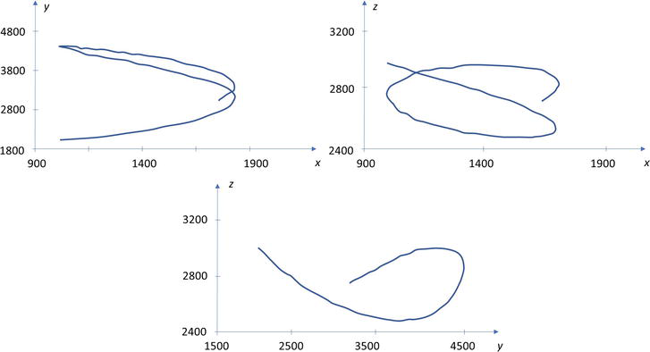
Figure 1.
The actual target trajectory in the CCS planes (
Because of a similar behavior of the actual components of three-dimensional state vector in each of the CCS coordinates, only the
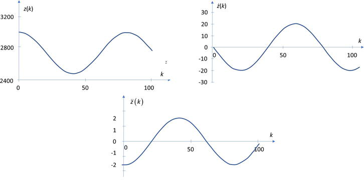
Figure 2.
The actual components of the three-dimensional state (position, velocity, and acceleration) in the z-CCS coordinate.
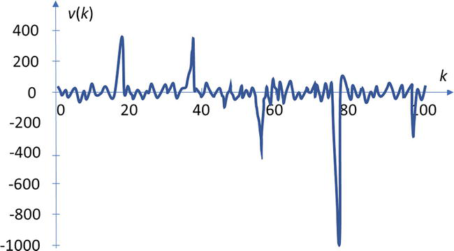
Figure 3.
Typical thick-tailed Gaussian glint noise record
The position measurements, in (1), are generated at each scan,
The filter-world equations of motion include only the linear discrete-time state-space representation with only the position measurement, in (1). Thus, the corresponding system matrices take the form
Here,
Radar observations commonly involve the range,
The implementation of the KF, robustified or not, requires the filter initialization, and a priori knowledge of the state and observation noises statistics. The optimal KF initialization, in (7), is based on the optimal estimates of zero-mean states, in (1), when the observations are not available. Thus, the adopted initial guesses,
Here, uncertainty in the initial three-dimensional state vector, in (1), is reflected in initial values of the covariance matrix,
The first-order statistics of state and observation noises are commonly zero-valued that is,
Particularly, by assuming
For the limiting case,
If a radar system measures in the SCS coordinates
Thus, the position measurement noise variance, in (2), in each of the CCS coordinates is given by the corresponding diagonal component of covariance matrix,
Performances of the next algorithms are compared: optimal KF (3)–(6), designated as A1; adaptive KF, combining the A1 filter with the Huber’s moving window M-robust algorithm to estimate noises moments, in (39), (42), (43), (52), (55), (56), (58) and (59), denoted as A2; M-robust estimate KF, in (35)–(38), denoted as A3; and adaptive M-robust estimate KF, combining the filter A3 and the Huber M-robust parameter estimator of unknown noises statistics in A2, denoted as A4. A filter adaptation to the unknown noise statistics requires to adopt the lengths of the corresponding sliding frames. A reasonable ad-hoc choices are
Simulation results, for each of the CCS coordinates, are analyzed using the cumulative estimation error (
with
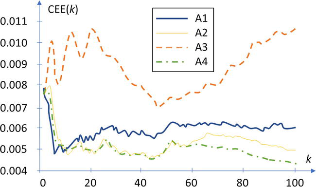
Figure 4.
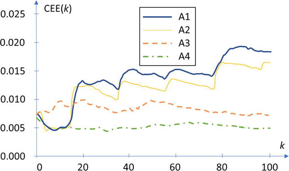
Figure 5.
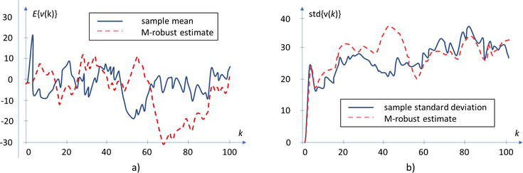
Figure 6.
Estimated measurement noise statistics comparison of sample mean and variance estimates upon Gaussian noise, and the algorithm A4 estimates upon thick-tailed Gaussian noise (
Finally, the adaptive robustified algorithm A4 provides the best results, representing an appropriate trade-off between tracking ability and robustness performance, suppressing efficiently outliers with a contamination degree less than thirty percent, (Figures 4 and 5). Also, the estimated noise statistics by the algorithm A4 upon the presence of outliers compare equally with the sample mean and variance estimates upon the absence of outliers, (Figure 6).
6. Conclusion
Since the Kalman filter has a computationally attractive recursive structure for real-time applications, it is widely used to solve the practical problems, involving system parameter identification, dynamic system state estimation, optimal and adaptive control, statistical signal processing, etc. In addition, numerous scientific and industrial measurements are analyzed, in the statistical sense, and the obtained results have indicated that the observations contain from five to ten percent of outliers, on average, due to incomplete measurements, meter and communication errors, errors in mathematical model, etc. In this sense, a thick-tailed Gaussian noise distribution is followed by the two types of impulsive noises, inducing innovation and observation outliers. The third type of outliers, named structural outliers, appears due to modeling errors, such as unmodeled system dynamics, time-varying model bias, computational errors, etc. Particularly, the thick-tailed normally distributed observations noise is presented in a maneuvering target tracking, due to the target glint inducing the innovation and observations outliers. Two characteristics of such data can be stressed. Firstly, there exists a high-intensity spiky character of the observations and, secondly, there is a clear low frequency, named the bright spot wonder, being produced by a slow drift in a target gravity center, due to changes in the target aspect. The low frequency can be efficiently suppressed in the tracking loop, but the glint spikes, representing the observation and innovation outliers, are stuck to the tracking loop. Moreover, a linear dynamic state space model is not adequate during a target maneuver, and such modeling errors induce structural outliers. However, since the Kalman filter is a linear signal processor, its performance can be very poor upon the outliers’ existence.
The basic objective of this manuscript is to design an appropriate Kalman filter modification that performs fairly well upon multiple outliers. It has been demonstrated, by a real-life maneuvering target tracking example, that the proposed adaptive M-robust estimate-based Kalman filter improves significantly the target estimation and tracking quality, being effective in suppressing multiple outliers with contamination degree less than thirty percent. Furthermore, the achieved improvement is at expense of the additional computational efforts, but usually not so demanded to preclude a real-time application. On contrary, the emphasized approximate Kalman filter may be more efficient than the least squares, or the optimal Kalman filter. Therefore, it may be used to solve the numerous engineering problems in which the Kalman filter, or least squares, is required. Furthermore, it may be also used as an alternative to the other adaptive techniques, involving discrete noise levels, variable state dimension, and interacting multiple model approaches, as well the observation distribution estimation. Further investigations may be directed to propagation of the error covariances upon a non-linear form of the state updates, as well as to the convergence, observability, and consistency analysis of the proposed approximate filter.
References
- 1.
Gelb A, Kasper J, Nash R, Price C, Sutherland A, editors. Applied Optimal Estimation, Analytic Sciences Corporation. Cambridge, MA: MIT Press; 1974. ISBN 9780262570480 - 2.
Grewal MS, Andrews AP. Kalman Filtering: Theory and Practice Using Matlab. Hoboken, NJ: Wiley; 2015 - 3.
Heijden F, van der Lei B, Xu G, Ming F, Zou Y, de Ridder D, et al. Classification, Parameter Estimation, and State Estimation: An Engineering Approach Using Matlab. Hoboken, NJ, USA: John Wiley & Sons, Inc; 2017 - 4.
Kovačević B, Đurović Ž. Fundamentals of Stochastic Signals, Systems and Estimation Theory with Worked Examples. Berlin: Springer; 2011 - 5.
Verhaegen M, Verdult V. Filtering and System Identification: A Least Squares Approach. Cambridge: Cambridge University Press; 2012 - 6.
Price C. An analysis of the divergence problem in the Kalman filter. IEEE Transactions on Automatic Control. 1968; 13 (6):699-702. DOI: 10.1109/tac.1968.1099031 - 7.
Hanlon P, Maybeck P. Characterization of Kalman filter residuals in the presence of mismodeling. IEEE Transactions on Aerospace and Electronic Systems. 2000; 36 (1):114-131. DOI: 10.1109/7.826316 - 8.
Albert AE, Gardner LA. Stochastic Approximation and Nonlinear Regression. Cambridge, MA: The MIT Press; 1967 - 9.
Saridis G, Nikolic Z, Fu K. Stochastic approximation algorithms for system identification, estimation, and decomposition of mixtures. IEEE Transactions on Systems Science and Cybernetics. 1969; 5 (1):8-15. DOI: 10.1109/tssc.1969.300238 - 10.
Stanković S, Kovačević B. Analysis of robust stochastic approximation algorithms for process identification. Automatica. 1986; 22 (4):483-488. DOI: 10.1016/0005-1098(86)90053-1 - 11.
Tsypkin, I. Adaptation and Learning in Automatic Systems. New York: Academic Press; 1971 - 12.
Mendel JM. Adaptive, Learning and Pattern Recognition Systems: Theory and Applications. New York: Acadamic Press; 2012 - 13.
Masreliez C. Approximate non-Gaussian filtering with linear state and observation relations. IEEE Transactions on Automatic Control. 1975; 20 (1):107-110. DOI: 10.1109/TAC.1975.1100882 - 14.
Masreliez C, Martin R. Robust Bayesian estimation for the linear model and robustifying the Kalman filter. IEEE Transactions on Automatic Control. 1977; 22 (3):361-371. DOI: 10.1109/TAC.1977.1101538 - 15.
Myers K, Tapley B. Adaptive sequential estimation with unknown noise statistics. IEEE Transactions on Automatic Control. 1976; 21 (4):520-523. DOI: 10.1109/TAC.1976.1101260 - 16.
Tsai C, Kurz L. An adaptive robustizing approach to kalman filtering. Automatica. 1983; 19 (3):279-288. DOI: 10.1016/0005-1098(83)90104-8 - 17.
Banjac Z, Kovačević B. Robustified Kalman filtering using both dynamic stochastic approximation and M-robust performance index. Tehnicki Vjesnik - Technical Gazette. 2022; 29 (3):907-914. DOI: 10.17559/tv-20200929143934 - 18.
Pavlović M, Banjac Z, Kovačević B. Approximate Kalman filtering by both M-robustified dynamic stochastic approximation and statistical linearization methods. EURASIP Journal on Advances in Signal Processing. 2023; 2023 (1):69. DOI: 10.1186/s13634-023-01030-1 - 19.
Barnett V, Lewis T. Outliers in Statistical Data. Chichester: Wiley; 2000 - 20.
Venables WN, Ripley BD. Modern Applied Statistics with S. New York: Springer; 2011 - 21.
Huber PJ, Ronchetti EM. Robust Statistics. Hoboken, NJ: Wiley; 2009 - 22.
Wilcox RR. Introduction to Robust Estimation and Hypothesis Testing. Amsterdam: Academic Press, an imprint of Elsevier; 2017 - 23.
Hampel FR, Ronchetti EN, Rousseeuw PJ, Stahel WA. Robust Statistics: The Approach Based on Influence Functions. Hoboken, NJ: Wiley; 1986 - 24.
Dutter R. Numerical solution of robust regression problems: Computational aspects, a comparison. Journal of Statistical Computation and Simulation. 1977; 5 (3):207-238. DOI: 10.1080/00949657708810152 - 25.
Hogg RV. Statistical robustness: One view of its use in applications today. The American Statistician. 1979; 33 (3):108. DOI: 10.2307/2683810 - 26.
de Menezes D, Prata D, Secchi A, Pinto J. A review on robust M-estimators for regression analysis. Computers & Chemical Engineering. 2021; 147 :107254. DOI: 10.1016/j.compchemeng.2021.107254 - 27.
Kovačević B, Milosavljević M, Veinović M, Marković M. Robust Digital Processing of Speech Signals. Berlin Heidelberg: Springer; 2017 - 28.
Boncelet C, Dickinson B. An approach to robust Kalman filtering. In: The 22nd IEEE Conference on Decision and Control. SA, TX, USA; 1983. pp. 304-305. DOI: 10.1109/cdc.1983.269847 - 29.
Kovačević B, Đurović Ž, Glavaški S. On robust Kalman filtering. International Journal of Control. 1992; 56 (3):547-562. DOI: 10.1080/00207179208934328 - 30.
Đurović Ž, Kovačević B. Robust estimation with unknown noise statistics. IEEE Transactions on Automatic Control. 1999; 44 (6):1292-1296. DOI: 10.1109/9.769393 - 31.
Chang G, Liu M. M-estimator-based robust Kalman filter for systems with process modelling errors and rank deficient measurement models. Nonlinear Dynamics. 2015; 80 (3):1431-1449. DOI: 10.1007/s11071-015-1953-0 - 32.
Gandhi MA, Mili L. Robust Kalman filter based on a generalized maximum-likelihood-type estimator. IEEE Transactions on Signal Processing. 2010; 58 (5):2509-2520. DOI: 10.1109/tsp.2009.2039731 - 33.
Zou Y, Chan S, Ng T. Robust M-estimate adaptive filtering. IEE Proceedings - Vision, Image, and Signal Processing. 2001; 148 (4):289. DOI: 10.1049/ip-vis:20010316 - 34.
Banjac ZD, Kovacevic BD, Milosavljevic MM, Veinovic MD. Local echo canceler with optimal input for true full-duplex speech scrambling system. IEEE Transactions on Signal Processing. 2002; 50 (8):1877-1882. DOI: 10.1109/tsp.2002.800415 - 35.
Banjac Z, Kovačević B, Veinović M, Milosavljević M. Robust least mean square adaptive FIR filter algorithm. IEE Proceedings - Vision, Image, and Signal Processing. 2001; 148 (5):332-336. DOI: 10.1049/ip-vis:20010594 - 36.
Kovačević B, Banjac Z, Milosavljević M. Adaptive Digital Filters. Berlin: Springer-Verlag; 2013 - 37.
Kovačević B, Banjac Z, Kovačević IK. Robust adaptive filtering using recursive weighted least squares with combined scale and variable forgetting factors. EURASIP Journal on Advances in Signal Processing. 2016; 2016 (1):37. DOI: 10.1186/s13634-016-0341-3 - 38.
Hewer G, Martin R, Zeh J. Robust preprocessing for Kalman filtering of glint noise. IEEE Transactions on Aerospace and Electronic Systems. 1987; AES-23(1) :120-128. DOI: 10.1109/TAES.1987.313340 - 39.
Woolcock SC. Target Characteristics. London: Technical Editing and Reproduction, Ltd; 1973 - 40.
Blackman SS, Popoli R. Design and Analysis of Modern Tracking Systems. Norwood, MA: Artech House; 1999