Forecast of Catastrophic Floods Based on Hydrodynamic Modeling: The 2013 Flood on the Amur River Case Study

Abstract

In 2013, a catastrophic flood occurred on the Amur River, caused by heavy rainfall throughout almost the entire basin. The floodplains of Blagoveshchensk, Khabarovsk, and Komsomolsk-on-Amur were flooded. Similar hydrological phenomena on the Amur occurred earlier (1954, 1972, and 1984), but they did not lead to catastrophic flooding. In the proposed manuscript, the authors investigated three issues: the causes of the 2013 flood, advanced hydrological forecast, and measures to prevent catastrophic flooding. For research, a hydrodynamic model of the Amur River section from Blagoveshchensk to the mouth was developed. Based on the analysis of model calculations, it was shown that some flood problems arose due to the construction of hydraulic structures in recent years (protective dams, bridges, and embankments) and a medium-term forecast scheme proposed.

1. Introduction

The rivers of the Amur basin, according to the nature of their water regime, belong to the type that is pronounced rain-fed. The share of rain-fed is 47–85%, snow 2–26%, and underground 9–31%.

The main phase of the water regime of the rivers of the Amur basin is rain floods observed in the warm season. The flood period lasts on average from 140 to 170 days (in the eastern and southern regions) to 110–150 days (in the northern and western regions). Floods are mainly observed from July to September. During the summer to autumn period, there are from 5 to 10 to 15 floods.

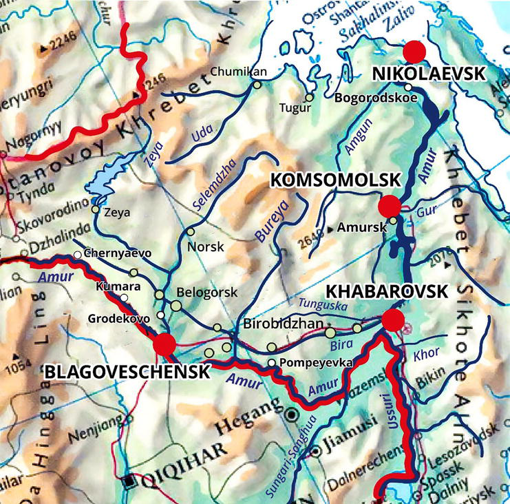
The large area of the basin and the diversity of conditions determine the existence of several flood sources of flood formation in the Amur basin. The main foci are the Upper Amur, Zeya-Bureya, Sungari, and Ussuri; see Figure 1 [1, 2]. Each of the listed sources can be the cause of the formation of a significant flood on the Amur; however, outstanding floods are formed as a result of the coincidence of the activity of two or more sources. For example, the flood of 1957 (35,500 m³/s) was formed in the Sungari (48%) and Zeya-Bureya (42%) sources. In 1958, the main source was the Zeysko-Bureya (62%), supported by the Upper Amur runoff (19%). In 1984 (32,900 m³/s), the Sungari (37%) and Zeya-Bureya (28%) sources were of greatest importance.

Figure 1.

The map of region under investigation.

The cause of the historic flood of 2013 for the entire Lower Amur (46,000 m³/s) was a high degree of synchronicity in the development and reach of flood waves from almost the entire territory of the Amur basin. The main role in the formation of the maximum discharge near Khabarovsk was played by the Zeysko-Bureya (30%), Ussuri (29%), and Sungari (24%) sources [3, 4].

The interval of maximum runoff modules for small and medium-sized rivers was 28.6–384 l/s km², i.e., the difference between the minimum and maximum values is fifteenfold, which confirms the wide variety of conditions for the formation of maximums. There is a group of rivers with very high values of peak flow modules (in the range of 200–400 l/s km²) located in the Zeya basin and the adjacent part of the Middle Amur.

This means reaching maximum values of approximately 1% probability of exceeding, observed in 1 year over a vast territory.

The main Amur high water, which led to the large-scale flood of 2013, began in July in the western part of the basin, where the main precipitation zones were located over the eastern part of the Zeya reservoir catchment, over the flat part of the Upper and Middle Amur and in the People’s Republic of China over the upper reaches of the Nonni River (Sungari basin).

The flow of the Upper Amur in 2013 was not extreme, although the water content of the Shilka and Argun in July and in the first half of August increased. As a result, the maximum levels of the Upper Amur were below dangerous levels.

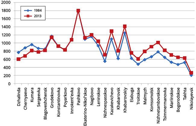
As it developed, the flood covered the Jewish Autonomous Region and the Khabarovsk Territory. The main Amur flood, moving downstream, accepted large amounts of water from the main southern tributaries – the Sungari (PRC), Ussuri, as well as numerous small tributaries [5]. Figure 2 shows a comparative description of two floods – the flood of 1984, the last of the observed catastrophic ones, and 2013. It can be seen that in the section of the Middle Amur from the city of Blagoveshchensk to the village, the Ekaterino-Nikolskoye flood developed in 2013, almost coinciding with the 1984 flood. Downstream, Amur levels in 2013 were significantly higher. Small tributaries of the Amur, both from the Russian and Chinese sides, were more abundant in 2013, since precipitation zones with good previous moisture continued to cover the basin when the main flood shifted.

Figure 2.

Comparison of maximum observed levels in 2013 and 1984.

Below the confluence of the Sungari, the level of the Amur was already more than a meter higher than in 1984. Both Sungari and Ussuri were more water-rich in 2013. The maximum discharge of the Sungari near the village of Jiamusi was 13,300 m³/s on August 31. Prior to this, the high-water content of the Sungari was observed only in 1998 (with a maximum flow rate of 16,200 m³/s), and the most abundant year in the lower reaches of the Sungari, 1960, was characterized by a flow rate of 18,400 m³/s. The share of the Sungari runoff in 2013 was about 30% of the Amur runoff near Khabarovsk during the period of highest flows, the share of the Ussuri runoff was about 16%, and the share of the Bureya runoff was about 6%. In 1984, Sungari gave about 18%, Ussuri – about 9%, Bureya – about 5%.

On a section of more than 1000 km (from the village of Nagibovo in the Jewish Autonomous Region to the village of Takhta in the Khabarovsk Territory), the maximum levels exceeded the historical maximums by 0.40–2.11 m. Moreover, the duration of such high levels (exceeding dangerous levels) amounted to about or more than a month in large cities, and the duration of flooding of the floodplain to depths of 2–4 meters was up to two and, in some places, more than months.

Water level near the city of Nikolaevsk-on-Amur (in the mouth area of the river Amur) was above the critical level in the period from September 10 to October 15, 2013.

2. Materials and methods

To analyze the causes of catastrophic flooding during the passage of a flood wave in August to September 2013, a hydrodynamic model (HDM) of the Amur River in the middle and lower reaches was developed. The model was calibrated for high flow rates (more than 10,000 m³/s).

The HDM was developed using the MIKE 11 computer program of the Danish Hydraulic Institute, using satellite images, digital elevation model (DEM) of the area, and Geographic Information System (GIS) of the Amur River [6, 7, 8, 9, 10, 11, 12].

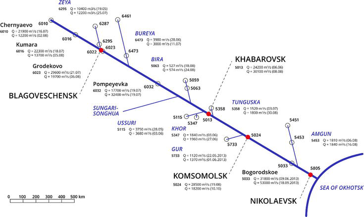
The modeling area is the Middle and Lower Amur from the village Chernyaevo (454 km above Blagoveshchensk city) to the mouth of the Amur River (Sea of Okhotsk). The model considers all the main tributaries that are significant in terms of runoff volume, including the rivers Zeya, Bureya, Sungari, Big Bira, Ussuri, Tunguska, Gur, and Amgun. Figure 3 shows the design scheme of the modeling area. The gauging station’s position corresponds to its distance from the mouth. For some gauging stations, the maximum discharges in 1958 and the dates of measurement are shown (except for gauging station 5733 “Snezhny,” for which data for 2013 was provided). The position of the largest human settlement areas is marked in red. The names of tributaries are shown in blue.

Figure 3.

Design scheme of the modeling area.

The modeling used cross-sections obtained from the results of field surveys carried out on morphological sections and from an updated digital terrain model (DEM) of the area (shuttle radar topography mission (SRTM) data) [11, 13, 14]. The digital model was clarified on the basis of cartographic materials of various scales, surveys conducted in previous years in the Blagoveshchensk and Khabarovsk cities area, survey materials, and pilot maps of 2006. Location of cross sections along the Amur River was designated in the locations of morphological sections, at existing (or previously existing) gauging stations, as well as in places requiring a detailed analysis of the hydraulic situation during high floods.

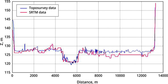
Cross sections formed on the basis of an updated DEM were corrected at the locations of morphological sections, considering the field survey results, which resulted in both systematic DEM errors and local satellite altimetry errors being corrected. Figure 4 shows an example of a comparison of cross-sections obtained using a DEM and as a result of surveys in 2014 at morphological Section 5 (village Belogorye).

Figure 4.

Comparison of the cross section obtained from the DEM and from the survey results (morphometric point 5).

The model accepts two types of boundary conditions, specified in the form of flow (hydrograph) and level time series – external and internal boundary conditions. Table 1 shows the location of the boundary conditions.

No.	Distance from source, km	Gauge number	Tributary	Settlement	Type of boundary condition
1	436	6010	Amur	Chernyaevo	External, Q
2	888	6295	Zeya	Belogorye	Inflow, Q
3	1152	6473	Bureya	Malinovka	Inflow, Q
4	2678	5453	Amgun	Guga	Inflow, Q
5	1607		Songhua	Jiamusi	Inflow, Q
6	1816	5115, 5347	Ussuri	Sheremetyevo+Khor	Inflow, Q
7	1696	5063	B. Bira	Birobidzhan	Inflow, Q
8	1874	5358	Tunguska	Arkhangelovka	Inflow, Q
9	2145	5733	Gur	Snezhnoye	Inflow, Q
10	2824		Mouth	Okhotsk Sea	External, Q

Table 1.

Boundary conditions adopted in the hydrodynamic model of the Amur River.

Historical hydrological data for the Amur River and its tributaries were used as initial data for modeling. To calibrate the model, 3 years were chosen – 1958, 1972, and 1984, which were closest in water content to the extreme year of 2013. It should be noted that the maximum flood in these years was formed on the Amur according to different scenarios. So, in 1958, the flood affected the upper and middle sections of the river, in 1972 and 1984 – middle and lower sections.

The main task was to obtain the most representative information for calibrating the hydrodynamic model, for which data on flow rates and levels for seven stations were processed: 6010 (Chernyaevo), 6016 (Kumara), 6023 (Grodekovo), 5012 (Khabarovsk), 5013 (Khabarovsk)), 5024 (Komsomolsk), and 5033 (Bogorodskoye). The most representative data seems to be g/s 5013 (Khabarovsk city station) and g/s 5024 (Komsomolsk) because they have observational data on flow rates and levels for the indicated 4 years.

Of the total number of tributaries flowing into the Amur River in the study area, tributaries located on the territory of the Russian Federation and the Sungari River, located in the People’s Republic of China, were taken into consideration. Gauging stations on tributaries were selected closest to the place where the tributary flows into the Amur River.

Initial data for all selected gauging stations were presented in the form of daily changes in levels relative to mark “0” (in cm) and absolute flow rates (in m³/s) for 1958, 1972, 1984 and 2013. Relative changes in levels were converted into absolute level marks.

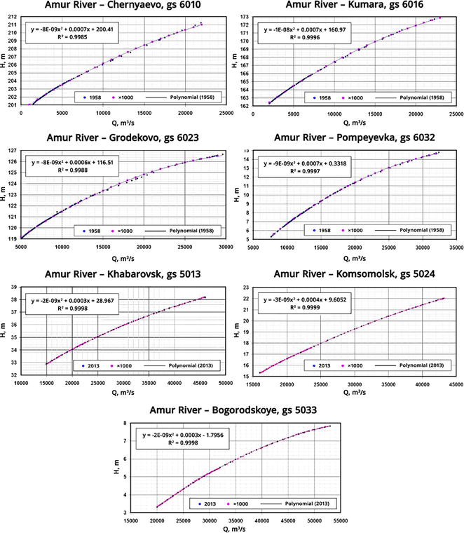
Based on the recalculated values, graphs of Q = f(h) were constructed for the period from 01.05 to 30.09. Graphs were built for all years for each g/s. Figure 5 shows Q = f(h) curves for all sections in which the hydrodynamic model was calibrated.

Figure 5.

Graphs of the Q = f(h) dependences at the calibration sections of the Amur River HDM.

Table 2 shows the observed data of the dependences Q = f(h) for maximum water discharges at the calibration sections of the Amur River HDM.

Gauge number	Distance from the source, km	Settlement	Maximum flow cubic m/s с	Maximum level, m
6010	436	Chernyaevo	21,900	211,25
6016	656	Kumaras	22,300	172,71
6023	903	Grodekovo	29,600	126,65
6032	1376	Pompeevka	32,400	82,05
5013	1862	Khabarovsk, Gaugest.	46,000	38,23
5024	2210	Komsomolsk	43,200	22,04
5033	2586	Bogorodskoye	53,000	7,84

Table 2.

Dependency data Q = f(h) for calibrating the model for maximum flow rates.

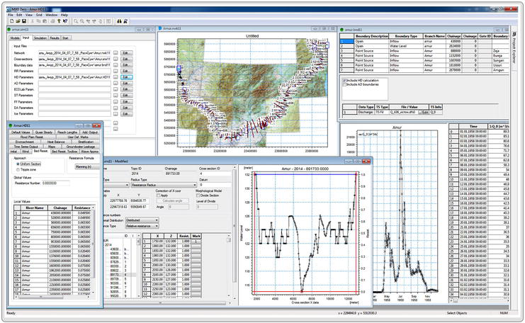
Figure 6 shows all open modeling editors windows in the MIKE 11: (1) modeling window, (2) river network, (3) boundary conditions, (4) inflow in 1958 to station 6010 chernyaevo, (5) cross-section, (6) hydrodynamic parameters (roughness and sediment conditions).

Figure 6.

Working windows of modeling editors in the MIKE 11.

3. Results and discussion

3.1 Results of hydrodynamic modeling of the 1958 flood wave

Using the developed hydrodynamic model, a calculation of the passage of the 1958 flood was performed [15].

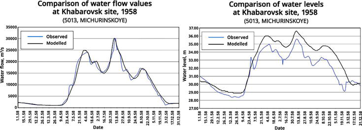
Figure 7 shows diagrams comparing observed data and data obtained as a result of modeling for two gauging stations.

Figure 7.

Comparative diagrams of the passage of the 1958 flood.

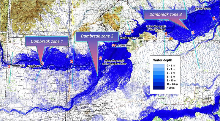
At high flow rates, the observed course of levels is significantly lower than the model one (by more than a meter). This indicates that there have been significant changes in the channel and bank morphometry of the Amur River in the Khabarovsk region. The reason for this was the construction of hydraulic structures that create backwater in the Amur River bed: Left bank coastal dams built by the Chinese side, channel gravel dams on the Pemzenskaya and Beshenaya channels, bridge across the Amur River in Khabarovsk. Due to exceeding the design level of coastal dams, flooding of the right-bank floodplain occurred in three regions of China (Figure 8).

Figure 8.

Dambreak zones during the 2013 flood.

3.2 Results of hydrodynamic modeling of flood wave movement based on data from the 2013 flood

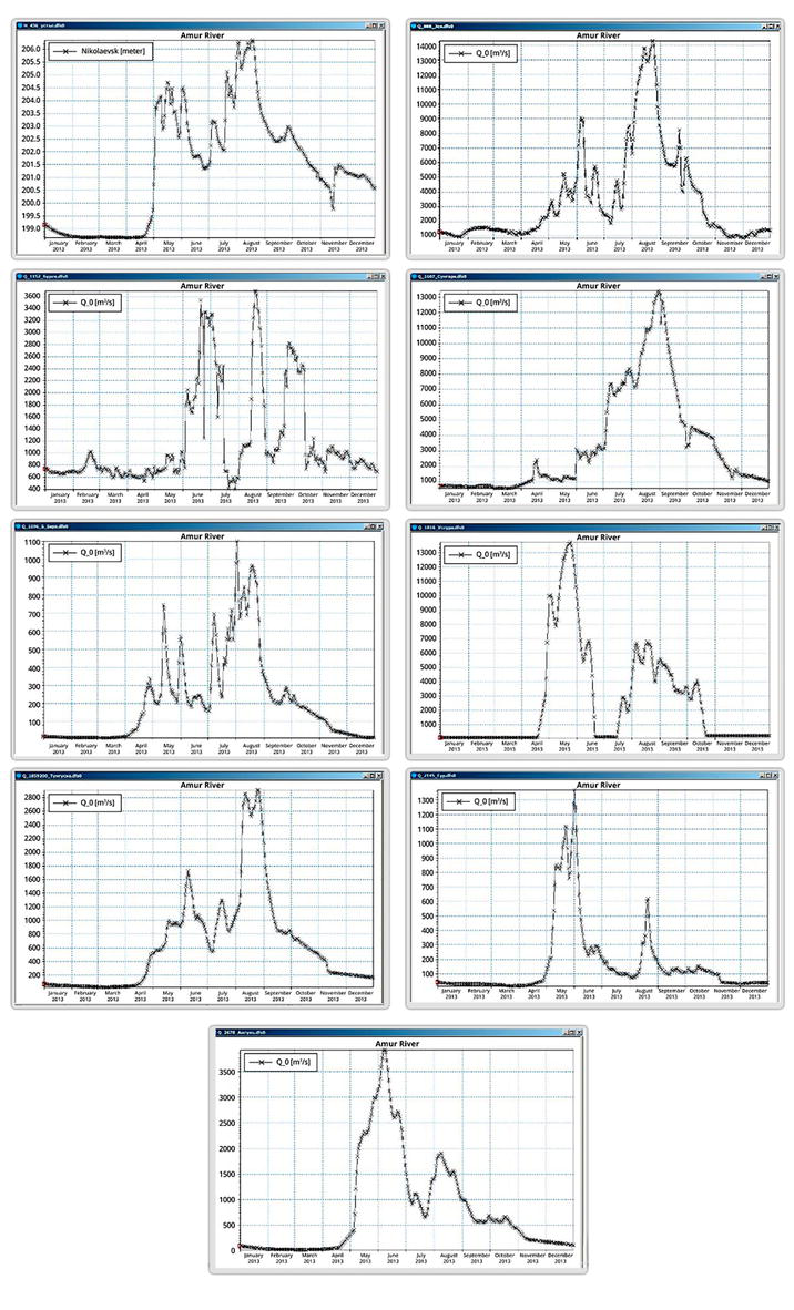
Using the developed hydrodynamic model, the calculation of the passage of the 2013 flood was performed [16, 17, 18]. Figure 9 shows inflow hydrographs.

Figure 9.

Hydrographs of inflow of the 2013 flood.

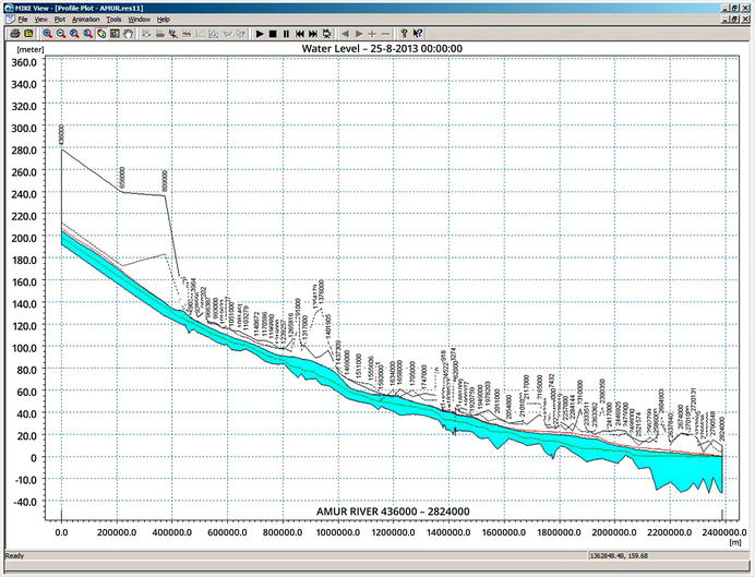
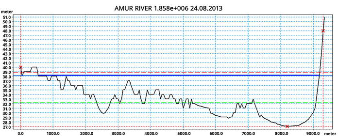
Figure 10 shows the longitudinal profile of the passage of the 2013 flood wave 9 days before the peak of the flood in Khabarovsk (maximum levels are indicated in red).

Figure 10.

Longitudinal profile of the passage of the 2013 flood wave.

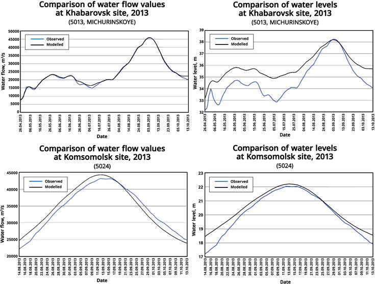
Figure 11 shows diagrams comparing observed data and data obtained as a result of modeling for two gauging stations. The discharges and levels fluctuations are given for part of the calculated time series during which the flood was observed.

Figure 11.

Comparative diagrams of the passage of the 2013 flood.

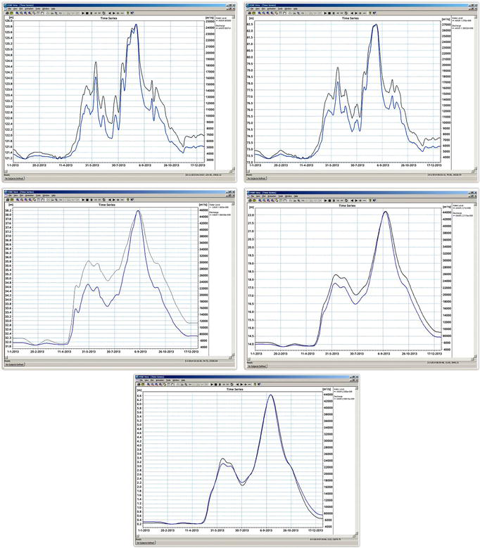
Figure 12 shows the results of calculations of Q/h at control stations g/s 6023 (Grodekovo), 6032 (Pompeevka), 5013 (Khabarovsk, city station), 5024 (Komsomolsk-on-Amur), and 5033 (Bogorodskoye) when passing flood wave 2013 along the Amur River.

Figure 12.

Results of calculations (flow rates and water levels) based on the hydrodynamic data of the 2013 flood.

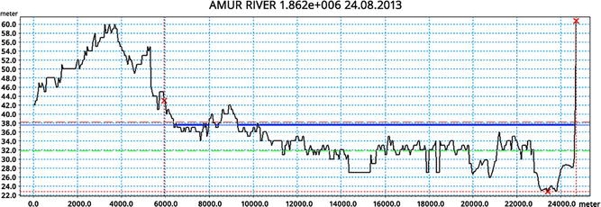
Figures 13 and 14 show the level fluctuations in the design sections of two cross sections of Khabarovsk city (before the railway bridge – g/s 5012, 4 km below the railway bridge – g/s 5013). Blue shows the water level line at the current moment, red shows the water line at the maximum level and green shows the water line at the minimum level in 2013. The height difference (difference in maximum values) was 38,9-38,1 = 0,8 m. In 1958, the height difference was 37,2–36,6 = 0,6 m.

Figure 13.

Range of water levels during the flood period of 2013 (g/s 5012).

Figure 14.

Range of water levels during the flood period of 2013 (g/s 5013).

3.3 Determination of the main parameters of the passage of high flood waters (time of arrival of the wavefront, wave crest, and time of wave decline to the flood level of 5% probability) in years of high-water content (1958, 1984, 2013)

In accordance with the methodological instructions of the Ministry of Emergency Situations, during the passage of high flood or breakthrough waves, it is necessary to determine the main parameters of wave propagation: the time of arrival of the wavefront, the wave crest, and the time of decline of the wave to a safe flood level of 5% probability. This allows timely implementation of measures to evacuate the population and livestock farms.

Table 3 and Figure 15 show the model parameters for the passage of the 2013 flood wave.

No.	Distance from the source, m	Parameters			Wave travel time, days
		Depth, m	initial level, m	Max. elevation flooding, m	Arrival of front	reaching maximum level	Decline to flood level 25% probability
1	436,000	7.3	199.1	206.4	20	26	28
2	656,000	6.6	161.5	168.1	22	27	30
3	809,000	3.3	136.2	139.5	23	29	32
4	883,000	5.6	124.7	130.4	24	31	33
5	903,000	4.4	121.5	125.9	15	31	36
6	993,000	4.0	110.1	114.1	16	33	38
7	1,051,000	4.4	103.6	108.1	17	33	39
8	1,183,730	4.1	91.2	95.4	18	34	41
9	1,291,000	8.4	81.0	89.4	19	35	42
10	1,376,000	9.7	72.9	82.5	20	35	43
11	1,511,000	3.0	56.2	59.2	21	36	44
12	1,634,000	7.0	48.4	55.4	13	40	63
13	1,858,000	6.2	32.6	38.8	8	44	88
14	1,862,000	6.0	32.2	38.2	0	44	89
15	1,949,000	6.2	26.8	33.0	4	45	92
16	2,054,000	4.2	21.7	25.9	10	49	95
17	2,117,000	6.6	17.1	23.7	11	51	97
18	2,210,000	8.1	14.1	22.2	12	52	99
19	2,310,000	11.3	8.2	19.5	14	52	101
20	2,417,000	7.0	5.7	12.7	14	53	101
21	2,498,000	6.5	2.4	8.8	15	54	102
22	2,586,000	6.4	0.3	6.7	17	56	104
23	2,701,000	3.2	0.1	3.3	9	57	105
24	2,776,000	1.8	0.0	1.9	9	56	106

Table 3.

Parameters of the passage of a high flood wave in 2013.

Figure 15.

Parameters of the passage of a high flood wave in 2013.

3.4 Flood zones during the passage of a flood wave during years of high water content (1958, 1984, and 2013)

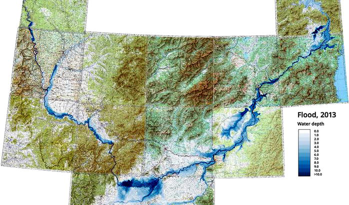
Based on the results of computer hydraulic modeling, flood maps of the Amur River valley were created for various forecast situations. These maps were constructed on the basis of a differential model obtained as the difference between the water level and relief marks. Positive values in such a model correspond to flood depths, and negative values correspond to the heights of the area above the water level. Negative values are discarded when plotted on a map.

Figure 16 shows a map of the flood depths of territories constructed based on the results of modeling the 2013 flood.

Figure 16.

Map of flood depths, built according to calculated data for 2013.

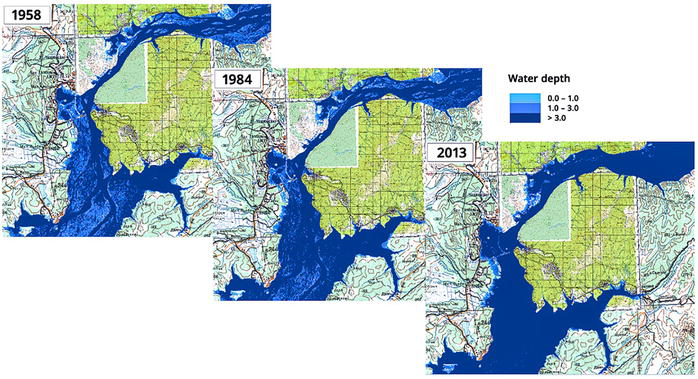
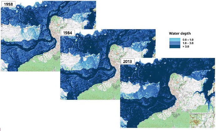
For the regions of the Khabarovsk and Komsomolsk cities on the Amur, detailed maps of flooding of territories were constructed, obtained from the results of modeling the floods of 1958, 1984, and 2013 (Figures 17 and 18).

Figure 17.

Maps of flood depths in the Khabarovsk region.

Figure 18.

Maps of flood depths in the area of Komsomolsk-on-Amur.

For selected areas (each with an area of 5932 km²) in the area of Khabarovsk and Komsomolsk on the Amur, the flooded areas of the territory were analyzed. The areas were calculated for the following flood depths: less than 1 m, from 1 m to 3 m, and more than 3 m. The area occupied by the Amur riverbed and channels during the low-water period for the site in the region of Khabarovsk amounted to 321.5 km², for the site in the region of Komsomolsk-on-Amur – 350 km². Data on the obtained estimated flood areas are given in Tables 4 and 5.

Flood depths	1958 г.	1984 г.	2013 г.
Up to 1 m	232,5	202,5	137,1
From 1 to 3 m	799,9	599,6	402,5
More than 3 m	1021,3	1437,7	1911,9

Table 4.

Estimation of flood areas in the Khabarovsk city area, km².

Flood depths	1958 г.	1984 г.	2013 г.
Up to 1 m	50,5	37,2	27,6
From 1 to 3 m	244	153,8	61,5
More than 3 m	524,6	661,2	843,4

Table 5.

Estimation of flood areas in the area of Komsomolsk-on-Amur, km².

3.5 Medium-term hydrological forecast based on hydrodynamic modeling

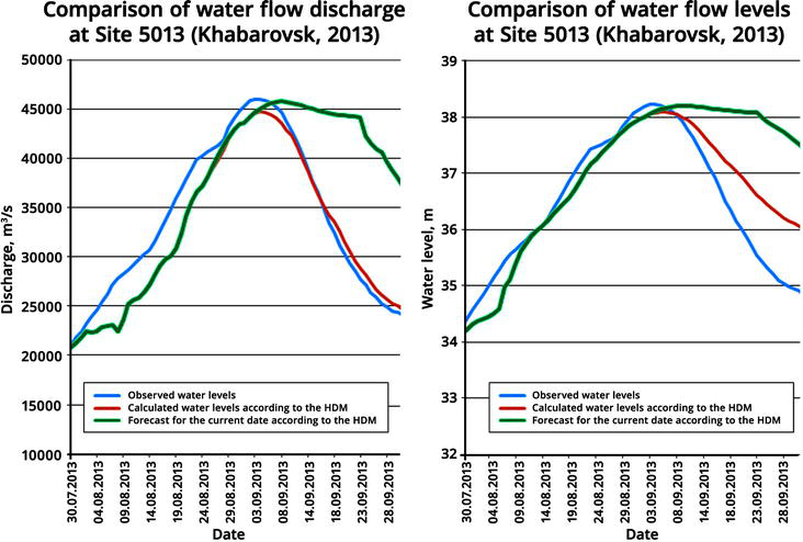
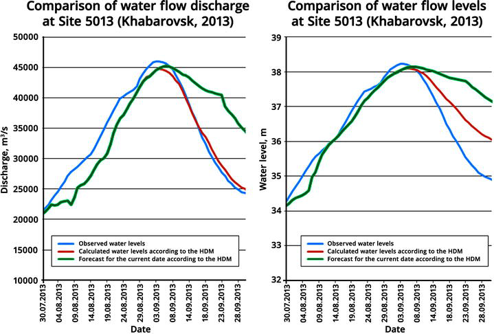
To demonstrate the predictive capabilities of the Amur River hydrodynamic model, model calculations of the 2013 flood were performed at various time intervals. In this case, the inflow forecast was carried out according to the principle: in the following days, the inflow will be the same as on the calculated date (settled hydrological regime).

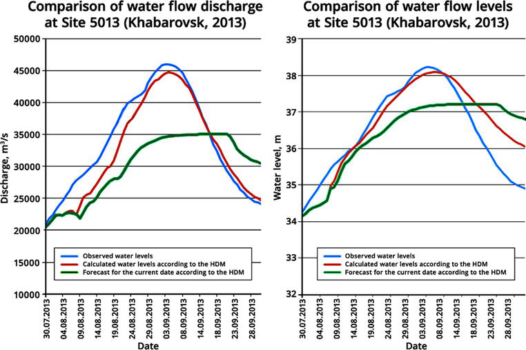
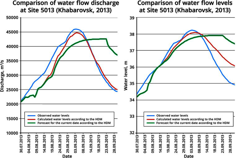
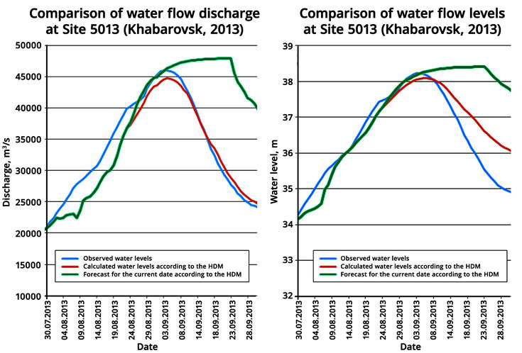
Figures 19–23 show three curves: observed water flows, obtained on the basis of modeling based on observed data (for the entire period) and made using predicted inflow data (see above). Calculations were performed for the following forecast dates: August 1 (33 days before the peak of the flood), August 8 (26 days before the peak), August 16 (18 days before the peak), August 22 (12 days before the peak), and August 25 (9 days before peak).

Figure 19.

Inflow forecast on August 1, 2013.

Figure 20.

Inflow forecast on August 10, 2013.

Figure 21.

Inflow forecast on August 16, 2013.

Figure 22.

Inflow forecast on August 22, 2013.

Figure 23.

Inflow forecast on August 25, 2013.

Figures 19–21 show how much the forecast curve (green diagram) differs from the observed curve (blue diagram). However, on August 22 (Figure 22), the predicted discharge already corresponds to the maximum observed discharge, but the maximum flow occurs at a later date. The final forecast diagram for August 25 (Figure 22) almost completely repeats the graph constructed using the observed data (the same result was obtained for water levels). The latter shows that the use of a hydrodynamic model of the Amur River would make it possible to do a fairly accurate forecast of the critical date and values of maximum flow rates and water levels 9 days before implementation (the peak of the catastrophic flood occurred on September 3, 4 and grew very quickly). The Khabarovsk Department of the Hydrometeorological Service provided a real forecast of the flood wave passage only 2 days before the peak, which did not allow the implementation of possible flood protection measures.

Thus, the timely use of the Amur River hydrodynamic modeling survey could reduce the risks of destruction during the catastrophic flood of 2013.

4. Conclusions

1. The hydrodynamic simulation model developed in the MIKE 11 software package adequately reflects the passage of high flood waters of 1958, 1984, and 2013 along the riverbed and floodplain of the Middle and Lower Amur, considering the flow of water through the main tributaries.

2. The results of the performed model calculations correspond to the observed data for water flows comparable to the maximum observed during the period of high floods in 1958, 1984, and 2013.

3. Based on the developed hydrodynamic model, short-term and long-term hydrological forecasts of rain floods in the Amur River basin, calculations can be made of a possible catastrophic hydraulic situation in the main settlements located on the Amur River.

4. The hydrodynamic model of the Middle and Lower Amur guarantees the issuance of the necessary final reports with the calculation of the main hydraulic characteristics of the river Amur bed and floodplain (water levels and flow rates, speeds, time of arrival of the wavefront, wave crest, and time of wave decline to a safe level, etc.). The model allows you to monitor a dangerous flood situation and perform a real-time short-term forecast of the occurrence of such a situation.

5. Using the developed digital terrain model and GIS project tools, possible flood zones can be quickly displayed on maps of various scales, and flood areas can be calculated for different depth ranges.

6. For the integral functioning of the model in a real-time mode, it is necessary to obtain flow characteristics, both for the main tributaries of the Amur River, formed on the territory of the Russian Federation (R. Zeya, R. Bureya, R. Ussuri, R. Amgun), and along the tributary of the River Songhua of the People’s Republic of China. It is necessary to restore the operation of gauging stations by measuring water flows, at least during periods of high floods.

7. The modeling results show that the current state of the river bed and floodplain of the Amur reduced its capacity. If the flood of 1958 were repeated under modern conditions, the water level in Khabarovsk would be 1–1, 2 m higher than observed in 1958.

Acknowledgments

This study was carried out under Governmental Order to Water Problems Institute, Russian Academy of Sciences, subject no 122041100222-7, FMWZ-2022-0001 and All-Russian Research Institute of Hydraulic Engineering and Land Reclamation subject no 68.31.00, FGUF-2022-0004.

References

1.Boikova KG. Floods on the Amur Basin Rivers, Voprosy Geografii Dal’nego Vostoka, Issue 5. Khabarovsk: Khab. Kn. Izd-vo; 1963. pp. 192-259. [in Russian]
2.Kim VI. The conditions for flood generation within the Amur River Basin. In: Voronov BA, Makhinov AN, editors. Research into Water and Ecological Problems of the Amur Region. Khabarovsk: Dal’nauka; 1999. pp. 66-69. [in Russian]
3.Dugina IO, Yavkina EN, Ageeva SA, Bol’sheshapova OV, Dunaeva IM, Efremova NF, et al. An Outstanding Flood on the Amur River in 2003 and its Characteristics, Abstract Book of the Plenary Meeting of the Seventh All-Russian Hydrological Congress; November 19-21, 2013, St. Petersburg. Vol. 2013. St. Petersburg: Rosgidromet; 2013. pp. 22-25 [in Russian]
4.Frolov AV, Georgievskii VY. The extreme flood event of 2013 within the Amur River basin. In: Proc. Joint Meeting on “Extreme Floods within the Amur River Basin: Causes, Forecasts, Recommendations”; January 20, 2014, Moscow. Moscow: Izd-vo NITs “Planeta”; 2014. pp. 5-39 [in Russian]
5.Bolgov MV, Alekseevskii NI, Gartsman BI, Georgievskii VY, Dugina IO, Makhinov AN, et al. The 2013 extreme flood within the Amur basin: Analysis of flood formation, assessments and recommendations. Geography and Natural Resources. 2015;36(3):225-233. DOI: 10.1134/S1875372815030026
6.MIKE. A modelling system for rivers and channels, reference manual. 2017. Available from: https://manuals.mikepoweredbydhi.help/2017/Water_Resources/MIKE_11_ref.pdf [Accessed: Dec. 18, 2023]
7.MIKE. A modelling system for rivers and channels, short introduction – Tutorial. 2017. Available from: https://manuals.mikepoweredbydhi.help/2017/Water_Resources/MIKE_11_Short_Introduction-Tutorial.pdf [Accessed: Dec. 18, 2023]
8.MIKE 11. A modelling system for rivers and channels, user guide. Available from: https://manuals.mikepoweredbydhi.help/2017/Water_Resources/MIKE11_UserManual.pdf [Accessed: Dec. 18, 2023]
9.MIKE ZERO. The common DHI user interface for project oriented water modelling, user guide. Available from: https://manuals.mikepoweredbydhi.help/latest/MIKE_Zero_General.htm [Accessed: Dec. 18, 2023]
10.MIKE VIEW. A Results Presentation Tool for MOUSE, MIKE URBAN, and MIKE 11, User Guide. Available from: https://archive.org/details/manualzilla-id-5838695 [Accessed: Dec. 18, 2023]
11.SRTM. Version 4, available from the CGIAR-CSI SRTM 90m) – Database. 2008. Available from: http://srtm.csi.cgiar.org [Accessed: Dec. 18, 2023]
12.ASTER. Global digital elevation model (ASTER GDEM) – Database. 2011. Available from: http://gdem.ersdac.jspacesystems.or.jp [Accessed: Dec. 18, 2023]
13.Botavin DV, Zavadsky AS. Experience in Constructing a Digital Relief Model of the Amur-Zeya Water Node Using Earth Remote Sensing Data. Stability and Dynamics of Erosion-Channel Systems. Moscow: Moscow State University Publishing House; 2012. pp. 94-100
14.Geoservices and geoportals for distributing remote sensing materials: Google Earth, Worldview alpha. Available from: https://earthdata.nasa.gov/labs/worldview/. http://kosmosnimki.ru/, http://glovis.usgs.gov/ and others. [Accessed: Dec. 18, 2023]
15.Boykova KG. Floods on the rivers of the Amur basin. In: Questions of Geography of the Far East. Vol. 5. Khabarovsk: Pedagogical University; 1963. pp. 192-236
16.Danilov-Danilyan VI, Gelfan AN, Motovilov YG, Kalugin AS. Catastrophic flood of 2013 in the Amur River basin: Formation conditions, recurrence assessment, modeling results. Water Resources. 2014;41(2):111-122
17.Gartsman BI, Mezentseva LI, Menovshchikova TS, Popova NY, Sokolov OV. Conditions for the formation of extremely high water content in Primorye rivers in the autumn-winter period of 2012. Meteorology and Hydrology. 2014;4:77-92
18.Makhinov A, Kim V, Shuguang L. Specifiks of the exstreme flood on the Amur river in 2013. In: Resourses, Environment and Regional Sustainable Development in Northeast Asia (Papers and Abstracts). Vol. 2014. Changchun, China: Northeast Institute of Geography and Agroecology, CAS; 2014. pp. 313-318
Written By
Alexander Buber and Mikhail Bolgov
Submitted: 21 December 2023Reviewed: 02 February 2024Published: 04 April 2024