Kalman Filtering Applied to Investment Portfolio Management

Abstract

Arbitrage is an approach to portfolio composition that times the selection of investment instruments based on deviations between price and true value, exploiting the expected movement of price toward true value. Pairs trading is an early form of statistical arbitrage, exploiting temporary deviations from equilibrium for instruments that tend to move together. To extend the potential investment, universe statistical arbitrage was extended to include several co-integrated instruments that display mean reverting model errors. A weakness of these methods is the possible breakdown of the observed relationships when the model error becomes a random walk, resulting in trading losses. Partial co-integration addresses this limitation by allowing for model errors that include both random walk and mean-reverting components. As both the mean-reverting and random walk components are non-observable, a Kalman filter approach is employed to estimate these system states. Partial co-integration is shown to outperform market returns and normal co-integration. Higher returns are observed during bear cycles, making it an attractive strategy to combine with bull market strategies. It is furthermore illustrated how partial co-integration can be further improved using convolutional neural networks to predict breakdowns in mean reversion and reinforcement learning to optimize the levels for entering and exiting trades.

1. Introduction

Kalman filtering is a method that enhances the estimation accuracy of uncertain observations by optimally combining the last available measurement with the best prior estimate [1]. The best new estimate is effectively calculated as a weighted average of the previous estimate, considering expected system behavior, and the last measurement. The weighting factors are moderated by the estimated uncertainty of the respective contributions, aiming to minimize the error between the estimate and the true value of the uncertain variable [1].

In the case of portfolio management investment, instruments must be selected to achieve an acceptable balance between risk and return. A key principle of portfolio management is diversification, exploiting the fact that the returns of different instruments are not perfectly correlated [2]. If only long positions are considered, an optimal portfolio will reside at the efficient frontier, which represents the highest return for a given risk, or the lowest risk for a given return [2].

A further improvement can be obtained by also considering short positions, allowing the hedging of risk by assuming a market neutral approach where the portfolio eliminates systematic risk, which is movement synchronous with changes in the overall market of available instruments [2]. In an ideal case, the portfolio will consist of a combination of long and short positions that are based on temporary mispricing observed in the market, with long positions taken in instruments that are underpriced and short positions taken in instruments that are overpriced. During the early stages of trading in financial instruments, it was possible to profit from such trades due to the lack of immediate information from all markets where the same instruments were traded, exploiting temporary differences in prices available in different exchanges. This was called arbitrage, which can be viewed as an approach to portfolio composition that takes long and short positions in the same instrument that is priced differently in different markets, guaranteeing a profit at zero risk [3].

As high-speed communication and information systems eliminated opportunities for this type of arbitrage, investment managers started to search for opportunities where the selection of investment instruments is based on deviations between current price and true value, aiming to exploit the expected movement of price toward true value. True value may be estimated based on observed statistical relationships between investment instruments over time; thus, the term statistical arbitrage was coined for a strategy that exploits deviations between current price and true value derived from long-term statistical relationships [4]. Pairs trading is a form of statistical arbitrage that involves the selection of two financial instruments that tend to move together [5]. For such instruments, when one is regressed in terms of the other, the model error tends to be mean reverting. An instrument that is known to be mean reverting can be exploited for profit: when the model error deviates beyond a set limit, a long position is taken in the instrument that is currently priced too low, given the price of the other, and a short position is taken in the instrument that is currently priced too high, based on the expectation that the model error will revert to its mean zero value [5].

Statistical arbitrage can be extended to include several co-integrated instruments. Rather than selecting only two co-integrated instruments, a group of co-integrated instruments is identified [6]. If the group is co-integrated and one of the instruments is regressed in terms of the others, the model error will be stationary and thus mean-reverting. If this model errors moves below a specified negative threshold, it is expected to return to its mean value of zero within a limited period, vice versa when the model error exceeds a positive threshold. Depending on the sizes and signs of the regression model coefficients, positions can be taken in each of the instruments so that the portfolio value will equal the model error [6]. Movement of the model error from a negative value back to zero will result in an overall profit for the portfolio. If opposite positions are taken for a movement of the model error from a positive value back to zero, a profit will once again be generated by the portfolio. Higher returns are observed during bear cycles, making statistical arbitrage an attractive strategy to combine with bull market strategies [7].

A weakness of this technique is the fact that the observed relationships may break down, causing the model error to behave like a random walk [7]. This may lead to large losses if the model error, after exceeding the predefined threshold, does not revert to the mean but continues a random walk away from zero until a stop loss threshold is exceeded. To counter this phenomenon, the concept of partial co-integration was introduced [7]. Partial co-integration allows for model errors that include both random walk and mean-reverting components. A Kalman filter approach is used to extract the mean-reverting and random walk components that cannot be observed directly. Trading signals are based on the mean-reverting component only, resulting in more frequent trades and thus more profit opportunities. Improvement of risk-adjusted returns generated by the partial co-integration strategy is enabled by the optimal selection of the Kalman filter gain [8]. Such a strategy can be shown to outperform market returns and normal co-integration.

The random walk component, which represents part of the returns that are generated when trades are executed, may however cause losses that will reduce overall portfolio profitability. A further improvement on the above approach is to predict the probability of a breakdown of the co-integrated relationship [9]. To generate information-rich features based on which changes in co-integrated behavior may be detected at an early stage, it is necessary to consider both time and frequency behavior of the price time series. Continuous wavelet transforms may be used for this purpose, transforming one-dimensional time data into a two-dimensional time-frequency space [9]. Convolutional neural networks are then applied to detect changes in the 2D behavior of the price series.

The portfolio optimization process can be based on reinforcement learning, which regards the portfolio as a Markov decision process [9]. Each possible portfolio composition is regarded as a system state. For each state, any of several actions can be taken to change the system to a different state; this represents new positions taken in the underlying instruments. For each state and action combination, a consequence is registered, this is, the profit or loss that results over the next period. By learning from past behavior through reinforcement learning, a model can be developed that makes an optimal decision for each possible system state. The objective function of the optimization process takes into account the probability that the co-integrated relationship may break down [9].

In this chapter, we review and compare the above approaches toward statistical arbitrage. It is shown that Kalman filters and partial co-integration can be successfully combined with deep learning and reinforcement learning to address the weakness observed in more traditional approaches to statistical arbitrage.

2. Statistical arbitrage and pairs trading

Arbitrage pricing theory (APT) was first suggested by Ross [3] to determine asset prices. Statistical arbitrage encompasses quantitative trading strategies with the following features: “(i) trading signals are systematic, or rules-based, as opposed to driven by fundamentals, (ii) the trading book is market-neutral, in the sense that it has zero beta with the market, and (iii) the mechanism for generating excess returns is statistical” [10]. Using market neutral strategies or long/short strategies to produce low-volatility investment strategies that take advantage of diversification across assets is very popular in the hedge fund industry [11].

Many statistical arbitrage strategies are focused on the concept of mean-reversion of security prices. The concept of mean-reversion trading is built on the assumption that a security’s high and low prices are only temporary and that the series will revert to a certain mean value over time [12]. While mean-reversion strategies are effective when price series are stationary, the price series of most securities are not stationary due to drifts caused by trends and momentum.

Nonstationary time series can be converted to stationary time series by differencing. To obtain a covariance stationary series, the series must be differenced by a minimum order of integration d, denoted $I\left(d\right)$. While single price series are seldom stationary, it is possible to obtain a stationary price series by creating a linear (weighted) combination of securities that exhibit a co-integrated relation. If the returns of two or more series are individually integrated of the same order and a linear combination of the series is integrated of lower order, the series are said to be co-integrated [13]. Some co-integration testing techniques include the Engle-Granger two-step method [14], the Johansen test [6], and the Phillips-Ouliaris test [15]. In contrast to the Engle-Granger method and Phillips-Ouliaris test, the Johansen test can be used to test multiple time series for co-integration.

Some forms of statistical arbitrage are pairs trading [16] and long/short strategies [17]. Pairs trading has been known in the quantitative finance community since the Mid-1980s [5]. It involves identifying two securities whose prices tend to travel together. The difference in prices is called the spread. Upon divergence of the spread beyond a defined threshold, the cheaper security is bought long and the more expensive one is sold short. When the prices converge back to their historical equilibrium, the trade is closed, and a profit is collected. The formalization of these concepts results in a quantitative trading strategy that exploits relative mispricing between two securities. Pairs trading can thus be regarded as a relative-value arbitrage strategy.

Zou et al. [18] pioneered pairs trading as a popular market-neutral trading strategy to exploit co-integrated relations that exist in the market between pairs of instruments. Vidyamurthy [19] suggested that APT can be used to detect tradeable pairs. Gatev et al. identified pairs to which statistical arbitrage could be applied using a minimum distance method to [16]. After obtaining securities that have a co-integrated relation, a certain hedge ratio must be determined for the pair; different approaches to calculate this hedge ratio have been investigated. Previous studies [20, 21] provide promising results employing the Kalman filter to determine the hedge ratio dynamically.

Gatev et al. [16] applied pairs trading to US CRSP securities for the period 1962 to 2002. They used sum of squared distances in normalized price space to rank all pairs in a 12-month formation period. They transferred the top 20 pairs with minimum distance metric to a subsequent 6-month trading period, entered a trade when the spread diverges at least two historical standard deviations from equilibrium, and closed it with the next zero-crossing, at the end of the trading period, or upon delisting. Using this approach, they achieved statistically and economically significant excess returns of 11% p.a., exhibiting low exposure to common sources of systematic risk.

3. Co-integration trading strategy

Pairs trading is profitable only if the spread between the securities is mean reverting, ensuring that it will return to zero within a reasonable period after diverging beyond the trading threshold. This requirement can be described in terms of the concept of co-integration. Two variables (in our case the prices of two instruments) are co-integrated if the error term resulting from regressing one in terms of the other is stationary [13]. Johansen extended this to an arbitrary number of variables involved in the regression [6]. A time series can be tested for stationarity using the Augmented Dickey-Fuller (ADF) [22] test. If a time series passes the test and is indeed stationary, a dependency is expected to exist between historic and future values: if previous values were above the mean, it is expected that upcoming values will move down toward the mean and vice versa.

The error term for a co-integrated set of variables can be described using an error-correction model or ECM [23]. The dynamics of one time series at a certain time point can then be described as a correction of the last period’s deviation from the equilibrium with the addition of possible lag dynamics. The advantage of using an ECM is that active predictions can be simply done by using past information.

To test for co-integration, the two-step procedure proposed by Engle and Granger [13] must be applied. First, a linear regression is run of the one series on the other. If the input and output variables $x_t$ and $y_t$ are co-integrated of order one, the error term ${\epsilon }_t$ of the regression will be weakly stationary (i.e., integrated of order zero). This is described by the following equation:

$$y_t=c_0+b{x}_t+{\epsilon }_t$$E1

Based on the work of Johansen [6], $x_t$ can be extended to a vector containing an arbitrary number of variables. The composition of the co-integration portfolio is dictated by the regression coefficients of the model. A portfolio can be obtained for which the combined value at any point in time corresponds to the model error or residual signal by investing into each instrument in proportion to the size of the regression coefficient.

A trading strategy must then be defined for opening and closing positions. The residual signal of each co-integrated set must be checked dynamically against a z-score that is calculated using the moving average ${\mu }_{\epsilon }$and standard deviation ${\sigma }_{\epsilon }$of the errors that were determined during the formation period:

$$z_t=\frac{{\epsilon }_t-{\mu }_{\epsilon }}{{\sigma }_{\epsilon }}$$E2

Trading signals are generated when $z_t$ exceeds predetermined thresholds; for instance, when $z_t=-2$, a long position is taken in the portfolio, while a short position is taken when $z_t=2$. The trade is closed when the spread has closed to a value of zero; alternative closing objectives may also be used.

Shares must be available for significant periods to extract reliable relationships based on which they can be tested for co-integration. A share must be available for the complete co-integration period to be considered for inclusion in a co-integrated set. For each group of instruments, a new model is extracted and tested for a sufficient level of co-integration on a periodic basis, using the h-values of the Engle-Granger or Johansen test. The resulting model error is tested for stationarity by applying the Dickey-Fuller test. A model is only accepted to compile a co-integrated portfolio if both tests are passed. In such a case, the same model is used until the conditions are satisfied for exiting the trade, that is, once the model error reaches a zero value. The periodic compilation of new models is then resumed until a new co-integrated relationship is found. The entry condition based on the z-value of Eq. (2) may be varied as part of the optimization process.

In the case of short positions, the negative values of the model coefficients are used to determine the effective positions in the shares. As model coefficients can have any sign, in most cases, portfolios consist of both short and long positions in the various instruments. As a result, the effective net investment position is mostly close to zero, given that long positions are partly offset by short positions in other shares.

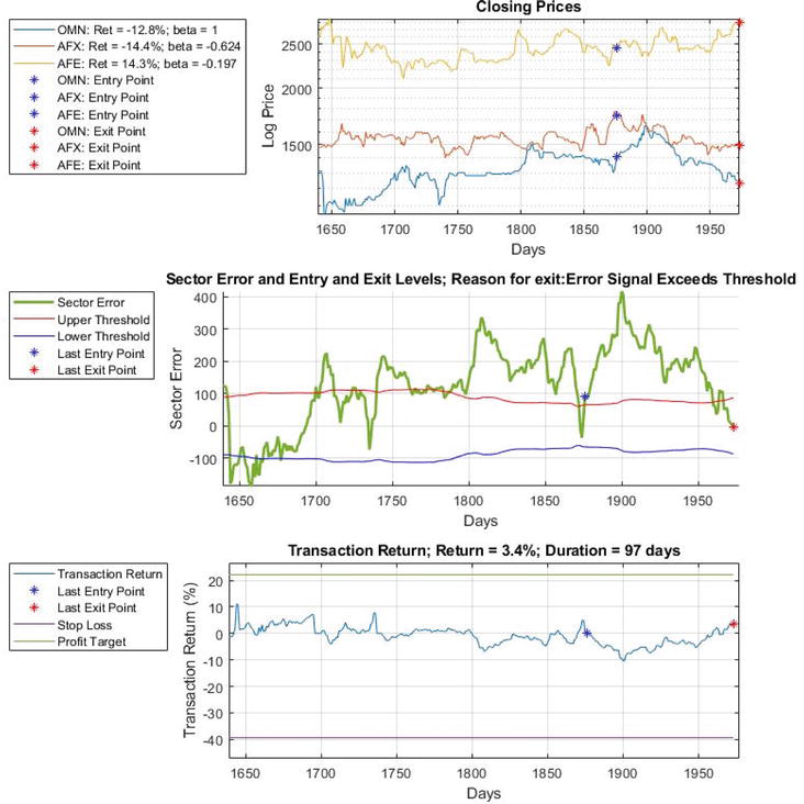
A typical trade that is entered and exited is illustrated in Figure 1 below. The closing prices of the shares forming part of the co-integrated set are displayed in the first graph. The second graph displays the error signal and the high and low thresholds that must be exceeded to trigger a trade. These thresholds vary over time as the level of volatility of the error signal changes over time. This is of specific relevance as the size of the error at the point of entering a position depends on the standard deviation of the error at that stage. The volatility of the underlying shares and thus of the model error is changing all the time, thus leading to widely varying standard deviations. This phenomenon is called heteroscedasticity and is often observed among financial instruments.

Figure 1.

Illustration of a typical co-integration strategy trade. Graph 1: Closing prices of a group of co-integrated shares. Graph 2: Error signal and trading thresholds, with entry and exit point indicated by *. Graph 3: Net return, stop loss, and profit target.

The position where a long trade is entered, once the error signal breaks through the upper threshold, is indicated by a blue star, and the red star indicates the point where the trade exits once the error signal breaks downwards through zero. The closing price graph displays the points where the trades occurred, as well as the returns produced by each share. The net return of the trade, the stop loss, and profit target levels as functions of time are displayed in the bottom graph—in this case, a loss was registered after entering the trade, as the error signal moved further above the threshold, but this turned into a profit by the time that the trade exits.

If the entire model error is used to trigger trades, entering at the threshold and exiting at zero, a guaranteed profit is made (excluding trading costs) each time that a position is taken and exited. An additional condition is however that the model error must indeed reverts to zero within an acceptable period. The model error could move away from zero indefinitely, should the co-integrated relationship between the instruments break down after a position was taken, as is typical for random walks. An unlimited loss can then be incurred on the position that was assumed, unless stop losses are implemented.

Another possibility is that a profit is shown before the zero-error level is reached, but that this turns into a loss before satisfying the zero-crossing condition for exiting the trade. A profit target may be set to exploit such profits by providing an alternative condition to exit the strategy on a profitable basis.

Clegg [24] found that for all shares forming part of the S&P 500 on the NYSE, the average proportion of variance attributable to mean reversion was 37%; thus, about 19% of price fluctuations in a given day would be attributable to the mean-reverting component. The average mean reversion component ρ was only 0.06, with ρ defined as the AR(1) coefficient of the mean-reverting price signal p_mr at time t and ${\epsilon }_{\mathit{mrs},t}$ the model error:

$$p_{\mathit{mr},t}=\rho p_{\mathit{mr},t-1}+{\epsilon }_{\mathit{mrs},t}$$E3

Both the proportion of variance attributable to mean reversion and the probability of persistence of mean reversion increase with ρ.

The model error (or spread) for a set of shares that satisfied the conditions for co-integration at the time of model extraction often tends to display behavior that is a combination of a random walk and mean reversion [8]. The random walk component of the error signal reduces the frequency of mean reversion, as it prevents the spread from reverting back to zero and may in some cases prevent the error signal from returning to zero at all, causing stop loss exits that erode profitability. These limitations suggested the need for a method that can differentiate between the mean-reverting and random walk components of the spread and thus the extension of the concept of co-integration to include partial co-integration.

4. Partial co-integration and the application of Kalman filtering

The weakness of trading strategies based on normal co-integration is the fact that the spread (or model error) is most often not mean reverting, but rather a combination of a random walk and mean-reverting behavior. The spread can be directly observed, using the respective share prices and the values of the extracted regression coefficients. The different error signal components contributing to the spread are however not directly observable.

Clegg and Krauss [7] proposed a solution that extends the model in Eq. (1) above as used by Engle and Granger. They did this by providing for an error that consists of a random walk element, a mean-reverting autoregressive element, as well as a stochastic component. As the different error signal components are not directly observable, Clegg and Krauss restated the model in state space to allow the unknown variables to be estimated using a Kalman filter approach.

A Kalman filter estimates a value for a stochastic variable that cannot be measured directly by using known relationships between observable variables and so-called system states that cannot be observed directly. In this case, the different states to be estimated from observations are the mean-reverting error component ${\epsilon }_{\mathit{mr},t}$ and the random walk error component ${\epsilon }_{\mathit{rw},t}.$ Eq. (1) is thus restated as follows:

$$y_t=c_0+b{x}_t+{\epsilon }_t=c_0+b{x}_t+{\epsilon }_{s,t}+{\epsilon }_{\mathit{mr},t}+{\epsilon }_{\mathit{rw},t}$$E4

The spread can therefore be written as:

$${\epsilon }_t=y_t-c_0-b{x}_t={\epsilon }_{s,t}+{\epsilon }_{\mathit{mr},t}+{\epsilon }_{\mathit{rw},t}$$E5

where the mean-reverting and random walk components of the spread can be written as:

$${\epsilon }_{\mathit{mr},t}=\rho {\epsilon }_{\mathit{mr},t-1}+{\epsilon }_{\mathit{mrs},t}$$E6

$${\epsilon }_{\mathit{rw},t}={\epsilon }_{\mathit{rw},t-1}+{\epsilon }_{\mathit{rws},t}$$E7

where it is assumed that the noise components of the system states are independent stochastic processes with zero means:

$${\epsilon }_{\mathit{mrs},t}\sim N\left(0,{\sigma }_{\mathit{mr}}^2\right)$$E8

$${\epsilon }_{\mathit{rws},t}\sim N\left(0,{\sigma }_{\mathit{rw}}^2\right)$$E9

For stochastic variables that cannot be measured accurately, a Kalman filter effectively estimates an accurate value by calculating a weighted average between the value estimated from previous observations and the value of the current observation, which is assumed to be uncertain [1]. The relative weights for the two contributions to the current estimation are based on the levels of uncertainty that exists about true values of the two contributions, derived from historic noise figures.

In general, the state space representation consists of two equations, a state equation and an observation equation, which may respectively be written as follows [24]:

$$Z_t=F_{t-1}{Z}_{t-1}+G_{t-1}{U}_{t-1}+W_{t-1}$$E10

$$X_t=H_t{Z}_t+V_t$$E11

where $Z_t$ is the state of the system that is not be directly observable (in this case the mean reverting and random walk contributions to the spread), while $X_t$ represents the observable parameters, in this case the share prices and resulting total spread. $U_t$ is a possible control input, which in our case is assumed to be zero. $F_{t-1}$ describes how the system changes from one sample period to the next in case of no external inputs $U_{t-1}$, while $W_t$ and $V_t$ are noise terms with covariance matrices $Q_t$ and $R_t$.

The Kalman filter algorithm makes it possible to determine the optimal estimate of the hidden states $Z_t$ based on previous observations and the assumed values of the system parameters. The Kalman filter equations are given as follows [24]:

$$P_t^{-}=F_{t-1}{P}_{t-1}^{+}{F}_{t-1}^T+Q_{t-1}$$E12

$$P_t^{+}=\left(I-K_t{H}_t\right)P_t^{-}{\left(I-K_t{H}_t\right)}^T+K_t{R}_t{K}_t^T$$E13

$$K_t=P_t^{-}{H}_t^T{\left(H_t{P}_t^{-}{H}_t^T+R_t\right)}^{-1}$$E14

$$Z_t^{-}=F_{t-1}{Z}_{t-1}^{+}+G_{t-1}{U}_{t-1}$$E15

$$Z_t^{+}=Z_t^{-}+K_t\left(X_t-H_t{Z}_t^{-}\right)=Z_t^{-}\left(1-K_t{H}_t\right)+K_t{X}_t$$E16

A crucial component of these equations is the Kalman gain matrix $K_t$, as it determines the influence that a new observation has upon the new estimate of the hidden states $Z_t$. This is clearly displayed in Eq. (15) above: the new system state $Z_t^{+}$ after a new observation $X_t$ is a linear combination of the state before a new observation $Z_t^{-}$ and the new observation $X_t$. For a very small Kalman gain (which represents the case where new observations are regarded as very uncertain), $X_t$ has a small weight, and thus, the new state estimation is almost the same as the previous state estimation, while for a high Kalman gain (which represents the case where there is a lot of confidence in new observations), the new state estimate is mainly determined by the new observation.

In the case of partial co-integration, the observable variables are the prices of the shares, while the different states to be estimated from observations are the mean-reverting error component ${\epsilon }_{\mathit{mr},t}$ and the random walk error component ${\epsilon }_{\mathit{rw},t}$. We write the observation equation and state equation, respectively, as follows, similar to the equations used by Clegg and Krauss [7]:

$$X_t=\left[\genfrac{}{}{0pt}{}{y_t}{x_t}\right]=\left|\begin{array}{ccc}b& 1& 1\\ 1& 0& 0\end{array}\right|\left|\begin{array}{c}{x}_t\\ {\epsilon }_{\mathit{mr},t}\\ {\epsilon }_{\mathit{rw},t}\end{array}\right|$$E17

$$Z_t=\left|\begin{array}{c}{x}_t\\ {\epsilon }_{\mathit{mr},t}\\ {\epsilon }_{\mathit{rw},t}\end{array}\right|=\left|\begin{array}{ccc}1& 0& 0\\ 0& \rho & 0\\ 0& 0& 1\end{array}\right|\left|\begin{array}{c}{x}_{t-1}\\ {\epsilon }_{\mathit{mr},t-1}\\ {\epsilon }_{\mathit{rw},t-1}\end{array}\right|+\left|\begin{array}{c}{\epsilon }_{\mathit{xs},t-1}\\ {\epsilon }_{\mathit{mrs},t-1}\\ {\epsilon }_{\mathit{rws},t-1}\end{array}\right|$$E18

where ${\epsilon }_{\mathit{xs},t-1},{\epsilon }_{\mathit{mrs},t-1},$ and ${\epsilon }_{\mathit{rws},t-1}$ are the innovations of the state variables $x_t$, ${\epsilon }_{\mathit{mr},t}$ and ${\epsilon }_{\mathit{rw},t-1}.$ The unknown parameters are the mean reversion parameter −1 < ρ < 1 and the variances of the mean-reverting and random walk processes σ_mr² and σ_rw². In the case of a steady state system, the unknown parameters are constants. These equations can be solved to estimate the values of the mean-reverting error and random walk error. Assuming that the mean reversion and random walk processes are independent, we can also define the proportion of variance attributable to mean reversion as [24]:

$$R_{\mathit{mr}}^2=\frac{2{\mathrm{\sigma }}_{\mathrm{mr}}^2}{2{\mathrm{\sigma }}_{\mathrm{mr}}^2+\left(1+\rho \right){\mathrm{\sigma }}_{\mathrm{rw}}^2}$$E19

It is then possible to solve for the unknowns as follows [24]:

$$\rho =-\frac{v_1-2v_2+v_3}{2v_1-v_2}$$E20

$${\mathrm{\sigma }}_{\mathrm{mr}}^2=\frac{1}{2}\left(\frac{\rho +1}{\rho -1}\right)\left(v_2-2v_1\right)$$E21

$${\mathrm{\sigma }}_{\mathrm{rw}}^2=\frac{1}{2}\left(v_2-2{\mathrm{\sigma }}_{\mathrm{mr}}^2\right)$$E22

where

$$v_k=\frac{{\left({\rho }^k-1\right)}^2+\left(1-{\rho }^{2k}\right)}{1-{\rho }^2}{\mathrm{\sigma }}_{\mathrm{mr}}^2+k{\mathrm{\sigma }}_{\mathrm{rw}}^2$$E23

The condition $2{\mathit{v}}_1-v_2=0$ is satisfied when ρ = 1, and as ρ < 1, the equations are well-defined. Each partial autoregressive series therefore has a unique parameterization. The above results can be used to obtain the following steady state solution for the Kalman gain matrix [24]:

$$K=\left(\genfrac{}{}{0pt}{}{\frac{2{\mathrm{\sigma }}_{\mathrm{mr}}^2}{{\mathrm{\sigma }}_{\mathit{rw}}\left(\sqrt{{\left(\rho +1\right)}^2{\mathrm{\sigma }}_{\mathrm{rw}}^2+4{\mathrm{\sigma }}_{\mathrm{mr}}^2}+\rho {\mathrm{\sigma }}_{\mathit{rw}}+{\mathrm{\sigma }}_{\mathit{rw}}\right)+2{\mathrm{\sigma }}_{\mathrm{mr}}^2}}{\frac{2{\mathrm{\sigma }}_{\mathit{rw}}}{\sqrt{{\left(\rho +1\right)}^2{\mathrm{\sigma }}_{\mathrm{rw}}^2+4{\mathrm{\sigma }}_{\mathrm{mr}}^2}-\rho {\mathrm{\sigma }}_{\mathit{rw}}+{\mathrm{\sigma }}_{\mathit{rw}}}}\right)$$E24

From the above equations, the unknown state variables can be determined as explained in the next section.

5. Partial co-integration trading strategy

After extracting the regression coefficients between the respective instruments and verifying for cointegration, the Kalman filter parameters are estimated using the equations provided in the previous section. This also allows the mean-reverting and random walk components of the spread to be estimated, as follows: the algorithm calculates the Kalman gain using ρ, σ_mr and σ_rw. Initially, it is assumed that ${\epsilon }_{\mathit{mr},t}=0$ and ${\epsilon }_{\mathit{rw},t}={\epsilon }_{s,t}$, that is, the spread, is regarded as a random walk. The algorithm then iterates through the remaining observations $X_t$. For each observation, the Kalman algorithm equations are used to produce the hidden state $Z_t$, that is, ${\epsilon }_{\mathit{mr},t}$ and ${\epsilon }_{\mathit{rw},t}$at that time.

Only the mean-reverting error component is used to trigger trades, rather than trading on the total error; not only will this increase the trading frequency—it will also prevent situations where indefinite losses are incurred due to long-term drift in the random walk component.

Hoffman [8] investigated the relationship between the values of $\rho \text{and}{K}_t$ and the profitability of the partial co-integration strategy. He extracted the value of the regression coefficients $\beta$ by using the techniques of Engle-Granger or Johansen and then optimized the profitability of the trading strategy profit in terms of the values of $\rho \text{and}{K}_k$. This enabled significantly improved net trading returns, as it allows the fraction of the error signal residing in the mean-reverting components to be controlled. He found that the value of the mean-reverting coefficient $\rho$ determines the fraction of the total co-integration error that resides in the random walk and the mean-reverting components, respectively; this is in line with the results of Clegg and Krauss [7].

As the underlying behavior of the instruments and the nature of their relationships tend to change over time, the following set of parameters should be optimized from time to time [8]:

1. The threshold for entering trades, defined as a multiple of error standard deviations.

2. The level of the stop loss, also defined as a multiple of error standard deviations.

3. The period over which the standard deviation of the error is measured.

4. Time window used to extract the co-integration relationships.

5. The level α of statistical significance for performing co-integration tests.

6. The profit target level.

7. Mean reversion coefficient ρ.

8. Kalman filter gain.

9. The minimum allowed value for the ratio between the standard deviation of the mean-reverting error signal and the standard deviation of the random walk error signal.

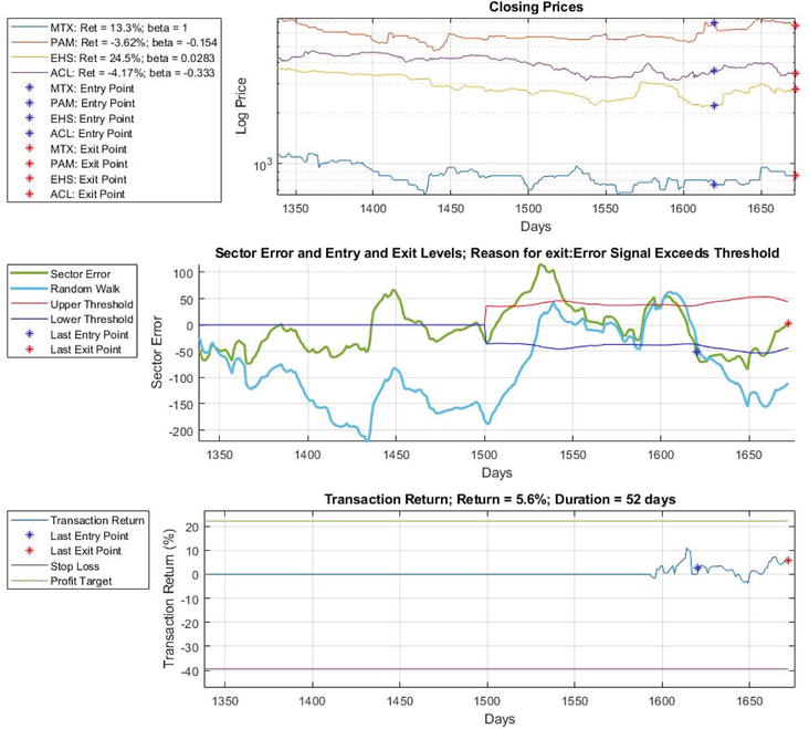
Figure 2 illustrates a typical trade that is based on partial co-integration. In the second graph, the error signal now consists of a mean-reverting and a random walk component; this is the main difference with the co-integration case in Figure 1. The trade is entered as the mean-reverting component breaks downward through the lower trading threshold and exits when this component returns to zero. The net return is the sum of the movements of both the mean-reverting and the random walk components. In this case, the trading profit was reduced as the random walk component performed a movement contrary to the movement of the mean-reverting component.

Figure 2.

Illustration of a typical partial co-integration strategy trade. Graph 1: Closing prices of a group of co-integrated shares. Graph 2: Mean reverting and random walk error signals and the trading thresholds, with entry and exit point indicated by X. Graph 3: Net return, stop loss, and profit target.

Hoffman [8] implemented a partial co-integration trading strategy on JSE shares by repeatedly extracting co-integrating share sets from 18 industry sectors for consecutive time periods. The available funds were divided equally between available trades from each of the 18 sector strategies to allow maximum diversification between all the available shares. This was repeated after each period where trading positions were assumed. Some sectors produced very few trades, while other sectors provided almost continuous trading opportunities.

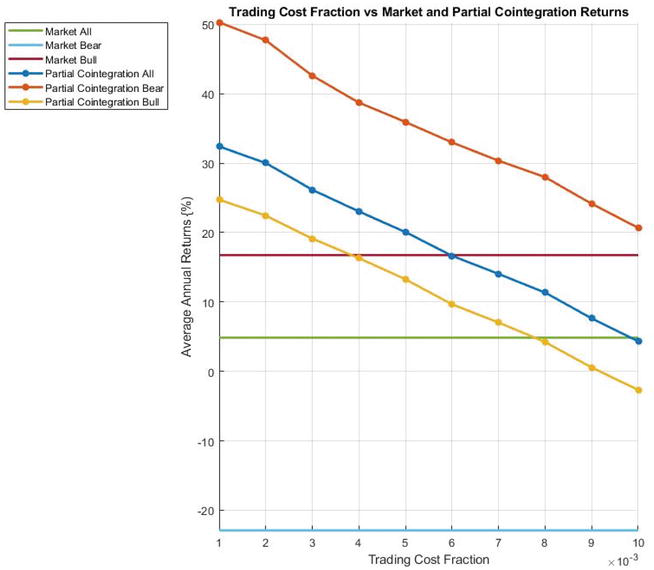
In line with Mashele et al. [25], he assumed a trading cost equal to 0.2% of the size of the trade upon entry and exit, resulting in a 0.4% total trading cost per trade. As statistical arbitrage is a high trading strategy, he also investigated the relationship between transaction cost and trading profits. The results are displayed in Figure 3. The expected reduction in profits can be observed as trading cost is varied from 0% to 1% per complete trade. A profit is still realized when transaction cost assumes its expected value.

Figure 3.

Average annual profits of the partial co-integration trading strategy on the JSE over the period 1996–2020 for different values of transaction cost.

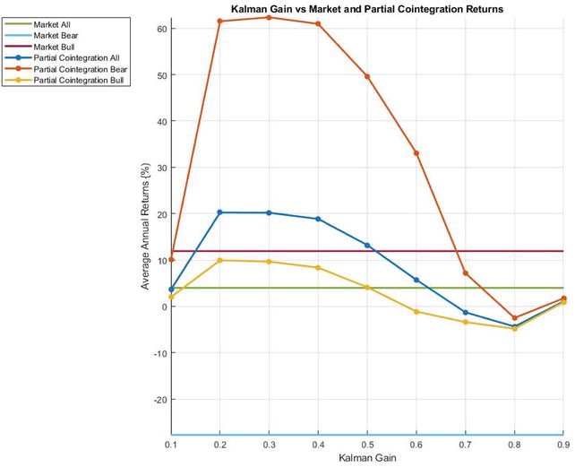
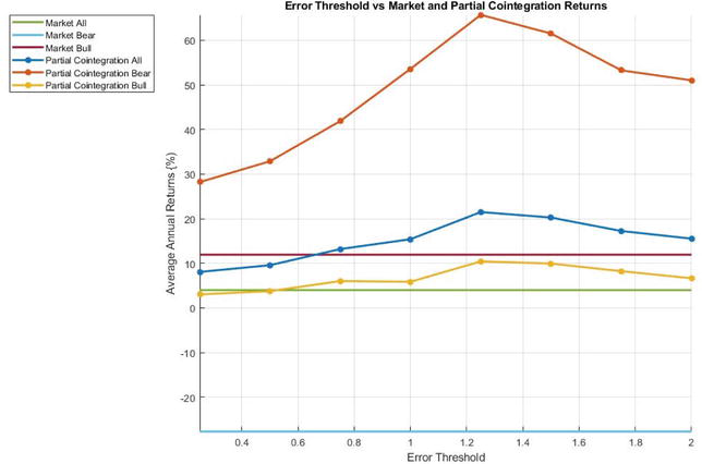
Figure 4 shows that the Kalman filter gain significantly influences trading profitability, with an optimal value of 0.7. Hoffman [8] also investigated the impact of trading threshold on performance, as the co-integration error signal levels where trades are initiated dictate the trading strategy. The trading parameter in this case is the value of z as reflected in Eq. (2) above, that is, the multiplier used to determine the error threshold in terms of the mean-reverting error signal standard deviation. As is clear from Figure 5, a value of 1.25 was close to optimal. A smaller number of trading opportunities exists for larger values, while the full profit potential of mean-reverting swings of the error signal is not exploited for smaller values. Repeating the calculations for the first and second halves of the available data set, respectively, indicated that the optimal values for the trading threshold are very similar for both data sets.

Figure 4.

Average annual profits of the partial co-integration trading strategy over the period 1996–2020 for different values of Kalman filter gain.

Figure 5.

Average annual profits of the partial co-integration trading strategy over the period 1996–2020 for different values of trading threshold multiplier.

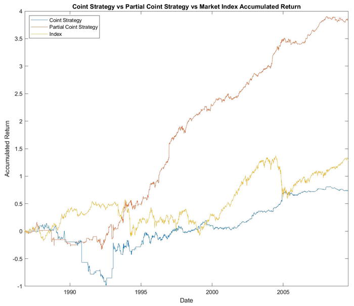
The trading strategy was implemented for the entire available date range. Subsequently, the annual profits (or losses) generated by the strategy as well as the average annual returns over the entire period were calculated. Figure 6 compares the accumulated returns generated over the period under investigation by the partial co-integration strategy against the market index and the co-integration trading strategy. The partial co-integration strategy far outperformed the market returns and normal co-integration returns. In addition, the returns generated by partial co-integration were more stable over time compared to market returns.

Figure 6.

Comparison of the accumulated returns of the market index with the co-integration and partial co-integration strategies.

To confirm this finding, Hoffman [8] also calculated the risk adjusted profits, using the Sharpe ratio [26]. The results are displayed in Table 1 [8].

	Market	Co-integration	Partial co-integration
All	4.96%	3.81%	22.32%
Low market return	−10.85%	5.78%	27.87%
High market return	19.71%	1.84%	17.15%
Bear cycles	−13.26%	12.54%	29.79%
Bull cycles	17.82%	−1.84%	17.05%
Sharpe ratio	0.15	0.09	0.87

Table 1.

Average annual returns during different parts of the market cycle [8].

The partial co-integration strategy achieved an overall annualized returns of 22.3% compared to market returns of 4.96%. The Sharpe ratio, which is a generally accepted measure of risk-adjusted returns, was 0.87 for partial co-integration compared to 0.15 for market returns. Over the evaluation period of more than 25 years, partial co-integration therefore significantly improved average returns, and reduced the volatility of returns. The normal co-integration strategy could not outperform the market in terms of either average returns or risk-adjusted returns, confirming that partial co-integration produces superior results compared to normal co-integration and outperforms market returns on a risk-adjusted basis.

It has been reported before [7] that statistical arbitrage tends to perform better during bear compared to bull markets. The performance of the co-integration and partial co-integration strategies were therefore separately evaluated for bear and bull markets on the JSE for the available period [8]. Bear and bull cycles were defined as years where market returns were, respectively, below or above a risk-free rate of return set at 2%. The average annual results are separately displayed in Table 1 for all market cycles, for the lower and upper halves of trading years sorted based on annual returns and for bear and bull cycles [8].

While the partial co-integration strategy performs similar to the market during bull and above average years, it outperforms the market by approximately 40% in terms of annualized returns during bear cycles and below average years. In contrast, the normal co-integration strategy outperforms the market during bear cycles and below average years but performs poorly during bull cycles and above average years [8].

The reasons for exiting co-integration and partial co-integration trading positions are displayed in Table 2. The partial co-integration strategy mostly exits positions because the mean-reversion error exceeded its threshold value, indicating that the trading strategy behaves as intended. Positions are exited because the profit target has been reached in about 25% of the cases, while very few positions exit because the stop loss was reached. In contrast, the co-integration strategy hits stop losses more often. The total number of trades is also much higher for partial co-integration compared to that for normal co-integration.

Number of exits/reason	No co-integration	Reached profit target	Reached stop loss	Same shares not available	Error signal exceeds threshold
Co-integration	0	395	34	13	17
Partial co-integration	0	527	10	7	1636

Table 2.

Reason for exiting trading positions [8].

Clegg and Krauss [7] provide results obtained for S&P 500 shares (representing about 80% of NYSE market capitalization) over the period 1990 to 2015, which is representative of mature markets that are expected to be more efficient than developing markets like the JSE. They found that compared to average annualized market returns of 9.6%, co-integration produced only 1.09% after transaction costs, while partial co-integration managed to beat the market with 12.34%. Partial co-integration also displayed a lower standard deviation than the market (8.24% compared to 14.99%). Due to its low average returns, co-integration achieved a Sharpe ratio of −0.37, while partial co-integration achieved 1.11 compared to a market value of 0.43. It would therefore appear that partial co-integration offers a viable statistical arbitrage trading strategy.

Clegg and Krauss [7] also compared partial co-integration with standard co-integration and with the market for different periods:

• Jan 1990–Mar 2001 (before the dotcom bubble);

• Apr 2001–Aug 2008 (after the dotcom bubble and before the global financial crisis);

• Sep 2008–Dec 2009 (during the global financial crisis);

• Jan 2010–Oct 2015 (after the global financial crisis).

They found that the excess returns achieved by partial co-integration were severely eroded since the global financial crisis. While the market achieved annualized returns of about 13% for both the first and last periods above, the returns on partial co-integration deteriorated from 22.3% to −2.76%. This is an indication that on mature markets, in contrast with developing markets, the use of sophisticated techniques has increased market efficiencies to a level where partial co-integration on its own can no longer offer practical benefits to large players who need to invest in large companies like those forming part of the S&P 500.

6. Prediction of structural breaks

The previous section described the influence of the presence of random walk components in the spread that is used as basis for statistical arbitrage. Structural breaks occur when the co-integration relationship breaks down, causing the model error to be dominated by the random walk component and thus to fade away from the historical means. The likely result of a structural break is that a stop loss is reached, reducing the profitability of the strategy. It is therefore beneficial to be able to predict the probability of a structural break before a trade is entered. Lu et al. [9] developed a structural break-aware pairs trading strategy (SAPT) that includes two phases: phase 1 predicts the probability of structural breaks, while phase 2 optimize the strategy, taking the probability of structural breaks into consideration.

Estimating the probability of structural breaks is modeled as a binary classification problem. The objective function tries to minimize the cross-entropy of all co-integrated pairs over the trading period. To increase the amount of useful information based on which the probability of future structural breaks can be estimated, both time and frequency content of the spread is used. The Fourier transform is the most common method to extract frequency content from time information. As it is however based on the assumption of an infinitely long time window, it is not suited to extract frequency information that can be dynamically updated as the nature of the spread changes. Instead, a continuous wavelet transform is applied to the model error (or spread) to obtain both time and frequency information about historical spreads that continuously updates as the underlying price signals change. Lu et al. [9] used the Ricker wavelet to extract such 2D wavelet features that are then fed into a CNN. CNNs have been proven to be very efficient at extracting features from images. The CNN applies a set of convolution filters to the input data, followed by ReLU activation functions and by maximum pooling to prevent overfitting and limit computational effort.

In addition, Lu et al. [9] used an LSTM model that is applied directly to the spread and the price signals. LSTM is one of the most successful recurrent neural network structures to model time sequences, as it can model both short- and long-term memory. The LSTM produces time domain features that are then combined with the time-frequency features of the wavelet CNN. The concatenated time and frequency domain features are fed into a stack of fully connected layers; this allows possible nonlinear interactions between the features to be learned. The output of the last layer is a scalar that models the probability of a structural break. The model is trained by minimizing cross-entropy, using dropout to prevent overfitting.

Lu et al. [9] performed experiments, using stock tick data for the top 150 companies on the Taiwan Stock Exchange Capitalization Weighted Stock Index (TAIEX) to ensure liquidity. They trained the system on a daily basis, using the first 150 minutes of each day to extract co-integrated pairs and trading for the rest of the day till 5 minutes before closing time. 75% and 25% of the data are, respectively, used for training and testing, and the last 20% of the training data are for validation. Their evaluation metrics are the True, Missed, and False detection rates for breakpoints, as well as the average delay between the actual and detected breakpoints.

They compared the following alternative approaches to detect structural breaks:

• a statistical 3-std threshold,

• the ADF test for stationarity,

• Bayesian change-point detection,

• Using LSTM to predict the spread,

• combining the use of the wavelet CNN in parallel with an LSTM network (SWANet).

They found that SWANet outperformed the alternative methods for structural breakdown detection. In Table 3, we provide the performance achieve by SWANet and the best of the alternative methods. The true detection rate can be further increased by increasing the tolerance for the accuracy by which a breakpoint must be detected—if the tolerance is increased from 20 to 70 minutes, the true detection rate increases from 47% to about 75%.

Performance measure	SWANet	Alternative methods
Missed detections	21%	27.4%
False detections	5.1%	34.6%
True detection rate	47.3%	24.4%
Average delay	17.3 min	22.3 min

Table 3.

Performance of SWANet compared to that of other structural breakdown detection methods.

7. Reinforcement learning for strategy optimization

In the section on partial co-integration, we have shown that trading profits are sensitive to the trading strategy that is employed. This suggests the use of a formal optimization approach to maximize profits. Lu et al. [9] developed a strategy to optimize the levels of the spread to open and close trades and the trading volume for trades. They modeled the strategy as a Markov Decision Process (MDP) and proposed a deep reinforcement learning model to optimize the strategy by deciding the optimal boundaries. Their deep Q-network builds a Q-function based on historical events and estimates the Q-values by incorporating risks (e.g., the probability of structural breaks) as well as transaction costs.

The inputs fed into the Q-network include the following:

• The current spread;

• Current positions in the respective instruments;

• The last actions, where the set of possible actions is defined as all possible sets of trading boundaries that may be used;

• The probability of a structural break;

• The risk that the market will close (e.g., at end of day), forcing the trade to be closed prematurely;

• The reward associated with each possible action, taking into consideration change in normalized prices, volume, and transaction cost.

The outputs generated by the Q-network include the entry level, stop-loss closing level, and normal exit level. The Q-network has the objective of maximizing the Q-value, defined as the sum of expected rewards:

$$Q^{\ast }\left(s_t,a_t\right)=E_{s_{t+1}}\left[R\left(s_t,a_t,s_{t+1}\right)+\gamma \underset{a_{t+1}}{max}Q\left(s_{t+1},a_{t+1}\right)|s_t,a_t\right]$$E25

where R is the reward, $Q^{\ast }$ is the maximum value of $Q$, and $\gamma \in \left[0,1\right]$ is a factor discounting the maximum possible Q-values in future. The Q-network uses a stack of several fully connected layers to learn behavior. To achieve the objective of approximating the target Q-value, the following loss function is defined:

$$\mathcal{L}\left(\theta \right)={\left(R\left(s_t,a_t,s_{t+1}\right)+\gamma \underset{a_{t+1}}{max}Q\left(s_{t+1},a_{t+1}\right)|s_t,a_t-Q\left(s_t,a_t\right)\right)}^2$$E26

where $\theta$ represents all the trainable parameters in the Q-network. These parameters are updated after each training iteration using the gradient of the loss function:

$$\theta \leftarrow \theta -\eta \mathcal{L}\left(\theta \right)$$E27

thus updating the Q-values as follows:

$$Q\left(s_t,a_t\right)\leftarrow Q\left(s_t,a_t\right)+\eta \left[R\left(s_t,a_t,s_{t+1}\right)+\gamma \underset{a_{t+1}}{max}Q\left(s_{t+1},a_{t+1}\right)|s_t,a_t-Q\left(s_t,a_t\right)\right]$$E28

where $\eta$ is the learning rate. The training is terminated when the loss function has reached a predetermined minimum value or when a predetermined maximum number of iterations is reached. The output is the action $a_t\in A$ that maximizes the Q-value, with $A$ the set of all possible actions. Comparing Eq. (26) with Eq. (15), a similarity is observed between the operation of the Q-network and the way in which the Kalman filter is used to update the system states, with the Q-values playing the same role as system states and the difference between the current and maximum Q-value playing a similar role as new observations.

The performance of this strategy was measured on the same set of Taiwanese stocks as for the breakpoint detection discussed in the previous section. The evaluation metrics included cumulative net profit, maximum drawdown, and Sharpe ratio. They compared a Q-network that uses only trading and stop-loss boundaries with a network that also factors in the probability of structural breaks, market closing risk, and transaction costs. The latter approach outperformed the former approach by about 15% over a trading period of 2.5 years, displaying the benefit of anticipating the occurrence of a structural break that will cause the spread to revert from mean reversion to a random walk. Predicting structural breaks had an even bigger impact on the reduction of risk, lowering maximum drawdown from 16.9% to 2%, and increasing the Sharpe ratio from 1.01 to 4.30 and the Sortino ratio from 1.41 to 13.18.

8. Conclusions

This chapter illustrated the applicability of the Kalman filter approach to the optimization of financial investment decisions. Financial markets represent a relevant example of a complex system of which the states can only be partly observed. As the quoted prices of instruments on an exchange are influenced by many factors, and as not all market players have access to the same information or may be restricted in terms of their speed of their reactions to new information, the true value of such instruments will not always correspond to the spot price. Statistical arbitrage intends to exploit temporary mispricings observed in the market by anticipating how the market will react to restore prices toward true values. The concept of co-integration was developed to provide a formal basis for pairs trading, which may be regarded as the initial form of statistical arbitrage. As the spreads that are created from sets of co-integrated instruments cannot be guaranteed to be mean reverting, co-integration had to be extended to provide for both mean-reverting and random walk system states, resulting in the concept of partial co-integration. This left the challenge to determine how the spread is divided between the mean-reverting and random walk components. The Kalman filter algorithm proved to be suitable to solve for these unknown system states, allowing the accuracy and profitability of trading strategies based on statistical arbitrage to be improved. Recent research has provided evidence that the Kalman filter method applied to partial co-integration can be complemented by using state-of-the-art AI methods, including convolutional neural networks and reinforcement learning. CNN classifiers help to address the weaknesses of partial co-integration by predicting when the random walk system state is likely to start dominating, thus avoiding possible loss-making trades. Reinforcement learning provides a systematic approach to make optimal selections for trading parameters, including the levels at which trades should be entered and exited. This provides a good example of how long-established methods can be combined with more recent innovations to meet the challenges of an ever-increasing complex world.

References

1.Kalman RE. A new approach to linear filtering and prediction problems. Transactions of the ASME -Journal of Basic Engineering. 1960;82((Series D)):35-45
2.Markowitz H. Portfolio selection. Journal of Finance. 1952;7(5):77-91
3.Ross SA. The arbitrage theory of capital asset pricing. Journal of Economics. 1976;13(3):341-360
4.Lo AW. Hedgefunds: An Analytic Perspective. Princeton: Princeton University Press; 2010. Available from: http://site.ebrary.com/id/10394786
5.Vidyamurthy G. Pairs Trading : Quantitative Methods and Analysis. Hoboken, NJ: John Wiley; 2004
6.Johansen S. Likelihood-Based Inference in Cointegrated Vector Autoregressive Models. Oxford: Clarendon Press; 1995
7.Clegg M, Krauss C. Pairs trading with partial cointegration. Quantitative Finance. 2018;18(1):121-138. DOI: 10.1080/14697688.2017.1370122
8.Hoffman A. Statistical arbitrage on the JSE based on partial co-integration. Investment Analysts Journal. 2021;50(2):110-132. DOI: 10.1080/10293523.2021.1886723
9.Lu J-Y, Lai H-C, Shih W-Y, Chen Y-F, Huang S-H, Chang H-H, et al. Structural break-aware pairs trading strategy using deep reinforcement learning. The Journal of Supercomputing. 2022;78(3):3843-3882. DOI: 10.1007/s11227-021-04013-x
10.Avellaneda M, Lee J-H. Statistical arbitrage in the US equities market. Quantitative Finance. 2010;10(7):761-782. DOI: 10.1080/14697680903124632
11.Thorp E. A Mathematician on Wall Street. 2000. Available from: http://www.wilmott.com/pdfs/080617_thorp.pdf
12.Bhave A, Libertini N. A Study of Short Term Mean Reversion in Equities. 2013. Available from: http://www.361capital.com/wp-content/uploads/2013/10/361_Capital_Study_Short_Term_Mean_Reversion_Equities.pdf
13.Engle RF, Granger CWJ. Co-integration and error correction: Representation, estimation and testing. Econometrica. 1987;55(2):251-276
14.Sjo B. Testing for Unit Roots and Cointegration. 2008. Available from: https://www.iei.liu.se/nek/ekonometrisk-teori-7-5-hp-730a07/labbar/1.233753/dfdistab7b.pdf
15.Phillips P, Ouliaris S. Asymptotic properties of residual based tests for. Econometrica: Journal of the Econometric Society. 1990;58(1):165. DOI: 10.2307/2938339
16.Gatev E, Goetzmann WN, Rouwenhorst KG. Pairs trading: Performance of a relative-value arbitrage rule. The Review of Financial Studies. 2006;19(3):797-827. DOI: 10.1093/rfs/hhj020
17.Thorp E. A Perspective on Quantitative Finance: Models for Beating the Market. 2003. Available from: http://media.wiley.com/product_data/excerpt/11/04700235/0470023511.pdf
18.Zhou ZZ, Kang S. Impact of the Shanghai-Hongkong stock connect on the performance of A-H pairs trading. In: Proceedings of the International Conference on Information Systems (ICIS). 2019. pp. 1-16
19.Vidyamurthy G. Pairs Trading: Quantitative Methods and Analysis. Hoboken, New Jersey: J. Wiley; 2004
20.Rudy J. Four Essays in Statistical Arbitrage in Equity Markets. Liverpool, U.K.: John Moores University; 2011
21.Chan EP. Algorithmic Trading : Winning Strategies and their Rationale. Hoboken, New Jersey: John Wiley & Sons, Inc.; 2013
22.Fuller WA. Introduction to Statistical Time Series. 2nd ed. New York: Wiley; 1996
23.Harlacher M. Cointegration Based Statistical Arbitrage. [Online]. 2012. Available from: https://stat.ethz.ch/research/mas_theses/2012/harlacher.pdf [Accessed: July 14, 2015]
24.Clegg M. Modeling time series with both permanent and transient components using the partially autoregressive model. 2015. SSRN 2556957.10.2139/ssrn.2556957
25.Mashele H, Terblanche S, Venter J. Pairs trading on the Johannesburg stock exchange. Investment Analysts Journal. 2013;2013(78):13-26
26.Sharpe W, Alexander G. Investments. Englewood: Prentice Hall; 1990
Written By
Alwyn J. Hoffman
Submitted: 12 January 2024Reviewed: 21 February 2024Published: 05 April 2024