Novel Approach for Turbulent Flow- and Onset Analysis

Abstract

It is a well-known fact that the matching of experimental data to turbulence models have hitherto not been successful. An example of this is the inability to theoretically predict the Re number at which turbulence onset (transition) occurs. In this paper, some advantages of adopting a “far-from-equilibrium” irreversible process analysis are demonstrated: To illustrate, one may at a single geometric point near a solid wall, compute conditions for mass conservation, 1st, and 2nd laws of thermodynamics – assuming either Newton’s viscosity law- or an alternative far-from-equilibrium fundamental model to be valid. While these conditions generally differ for various flows, it is observed that these conditions numerically match each other at Re_D around 2300 for a fully developed pipe flow, or at Re_x between 5 × 10⁵ to 3 × 10⁶ in a developing flat-plate boundary layer flow. This suggests that turbulence onset can be correctly predicted using the novel approach. Criteria and recommendations for experimental flow measurements, i.e. testing conditions, within a proposed far-from-equilibrium zone (e.g. viscous sublayer) is discussed as well.

1. Introduction

According to [1], the following question is posed: “Why is turbulence so hard to solve?” It is stated that: “An example of why turbulence is said to be an unsolved problem is that we can’t generally predict the speed at which an orderly, non-turbulent (“laminar”) flow will make the transition to a turbulent flow.” Perhaps, an understanding of the mechanisms resulting in the onset of turbulence is a key issue for the understanding.

The turbulent flow differs from a well-ordered laminar shear flow [2, 3, 4, 5, 6, 7], and for a wall-bounded turbulent flow, several near-wall regions appear. Moreover, the kinetic energy dissipation is a rudimentary quantity, associated with the far-from-equilibrium process, and this increases drastically with the onset of turbulence.

A theory that in the following is referred to as the “Classical Turbulence Theory (CTT),” has been developed since the early 20th century. Originally, turbulence was considered a random process [8], involving swirling or rotating fluid elements, commonly referred to as “eddies” or “vorticities.” Through the last 50 years, many researchers have focused their interest on the transition and the flow behaviour in the innermost region of a turbulent boundary layer, e.g. coherent structures, bursts, and sweeps [3, 9, 10, 11, 12, 13, 14].

The Navier-Stokes relations are originally based on the continuum hypothesis [3] and assuming the flow processes to be governed by Newton’s viscosity law (a near-equilibrium irreversible thermodynamic process) [15]. This set of relations can be excellently applied on laminar flows, however, this set of relations is also assumed to be valid in turbulent flows [15, 16, 17, 18, 19, 20, 21]. Commonly, in CTT, a Reynolds decomposition is made, allowing for a simplification of the Navier-Stokes relations. The ensuing Reynolds-averaged Navier-Stokes relations incorporate new (unknown) quantities referred to as “Reynolds Stresses.” This is the so-called “closure problem” of turbulence which requires a modelling of the stresses to account for temporal- and spatial scale influence.

In CTT, a constant shear stress across the inner part of the turbulent boundary layer is assumed. This represents an empirical assumption: In short, it is assumed (cf. Hinze [22] p. 468) that both viscous and turbulent interactions contribute to the shear stress, a sum which is constant across all these regions, cf. [5] (and discussed partly in Section 2.3). According to Panton [3] (p. 720): “At the wall itself, the stress ${\tau }_0$ is 100% viscous shear because the fluctuation must vanish. Through the buffer layer $\tau$ decreases while the Reynolds stress $-\rho \overline{u_1{u}_2}$ increases. At the outer edge of the buffer layer, the stress is essentially all turbulent Reynolds stress and is equal to the wall value ${\tau }_0$. The Reynolds stress continues to be constant through the overlap region.” According to [5], the viscous processes have a negligible influence in the log-law region. The value assigned to the Reynolds Stress in the log law region is $-\overline{u_1{u}_2}={\left(U^{\ast }\right)}^2$, cf. Section 2.3.

A novel approach to analyse turbulent flows is presented here, see [23, 24], and it is based on the onset of a far-from-equilibrium [25, 26, 27] fundamental process at a specific threshold condition. Hence, a similar large-scale flow behaviour is obtained as in the CTT approach. However, some differences may be noted:

• The novel approach puts focus on the fundamental model as responsible for the build-up of the near-wall zones; viscous sublayer, buffer layer, overlap region/log-law region, and outer region of a turbulent wall boundary layer, which occurs due to a kinetic energy dissipation near the solid wall.

• On the nature of here so-called “visible swirls” or “visible eddies” (as all fluid elements within the novel approach falls under the category of “eddies”), the novel approach suggests conditions where these may form – however, the influence of these swirls and eddies appear to be limited when computing the net kinetic energy dissipation.

In this paper an attempt is made to discuss the application of the novel approach. Section 2 presents a simplified discussion on how a far from equilibrium process differs from the traditional continuum approach. Then, a thorough description of the novel fundamental far-from-equilibrium process is given and applied in computations of the shear stress variation in a fully developed pipe flow.

In Section 3 the discussion is extended to the analysis of turbulence onset (transition) in pipe flows. Noteworthy is that for the novel approach, it is possible to extract the onset condition by considering the mass conservation and 1st and 2nd laws of thermodynamics at a specific Re_x position along a flat wall, or a specific Re_D flow condition for a pipe flow. Both these Re numbers agrees well with established experimental data.

Section 4 is devoted to a discussion on the planning of near-wall experiments and simulations, incorporating far-from-equilibrium considerations.

2. Novel approach

2.1 Comparisons between irreversible continuum- and far-from-equilibrium processes: A summary of differences

A difference between continuum CTT approach and the far-from-equilibrium process, grossly simplified, is the following:

• For the continuum processes the principle of local equilibrium is applicable, that is at all positions $\left(y_1,y_2,y_3,t\right)$, quantities like temperature, pressure, density all have a unique value. These quantities are defined locally in an elemental volume with a large enough number of molecules allowing for the principles of thermodynamics to be valid, i.e. the viscous dissipation of a soft gradient shear-flowing Newtonian fluid can in an elemental volume be strictly computed by knowledge of the local flow gradient.

• In the far-from-equilibrium process, there is an overall mechanism, which controls the global behaviour. Often ordered structures (e.g. waves) are created, referred to as “dissipative structure,” and results in a significantly larger net entropy generation. One such mechanism is the MEP (Maximum Entropy Production principle) [28], which organises local flow behaviour. The build-up of viscous sublayer, buffer layer and log-law region are results of this organisation, see [23]. An important aspect of this condition is that – in contrast to continuum processes – a specific gradient in the flow does not necessarily translate into a kinetic energy dissipation [23, 24]. To illustrate, a flow gradient within the viscous sublayer, which is considered a saturated kinetic energy dissipation zone, the far-from-equilibrium model will give a strict number on the kinetic energy dissipation per unit volume. However, in zones where “defects” are located, or “clouds of defects,” the local condition with flow gradient can have any local kinetic energy dissipation, from 0 up to, but not exceeding, the kinetic energy dissipation for a corresponding saturated condition. This aspect of a far-from-equilibrium process is important, as it allows the overall invisible MEP process to organise the dissipative structures, while less dissipative zones will immediately adapt to the local conditions (without any violation of the principle of mass conservation). At low-dissipative zones, the flow may switch back to continuum mode. (Nonetheless, the return to continuum may incorporate some hysteresis phenomena, as discussed in [24].)

2.2 Method

The proposed far-from-equilibrium model valid after turbulence onset, is in [23] expressed in terms of a kinetic energy dissipation $\frac{\mathrm{d}{\left(\mathrm{ke}\right)}_{\mathrm{res}}}{\mathrm{d}t}=C_A\frac{\mathit{\rho L}}{\delta }{U}_{\text{slip}}$, which is an Eulerian expression.

The background stems comparing the original concept of a solid with that of a fluid: A solid beam obeys the rules of shear stress vs. strain, principally like a laminar fluid flow where instead of strain the strain rate is introduced.

Consider a glass solid in the shape of a beam, but where a far-from-equilibrium impact of, say, a bullet, results in a bullet hole in the beam together with a creation of a spider-network-type of fractures around the hole. Some immediate observations on the far-from-equilibrium impact process can be observed: First, the concentration of fractures decrease with increasing distance from the bullet hole, and second, the appearance of the spider-web-type of fractures is not at all random – an ordered dissipative structure may have been active in the creation of the web of fractures around the bullet hole.

Now, if applying the same bending operation of the bullet-fractured beam, with the aim of recording the overall shear stress vs. strain, the results will be completely different. A solid mechanics scientist would state that this analysis is invalid, and if attempting to understand the solid mechanics behaviour of a fractured beam, it would be of more interest to study the resulting slippage along a single fracture and connect the slippage with some kind of friction.

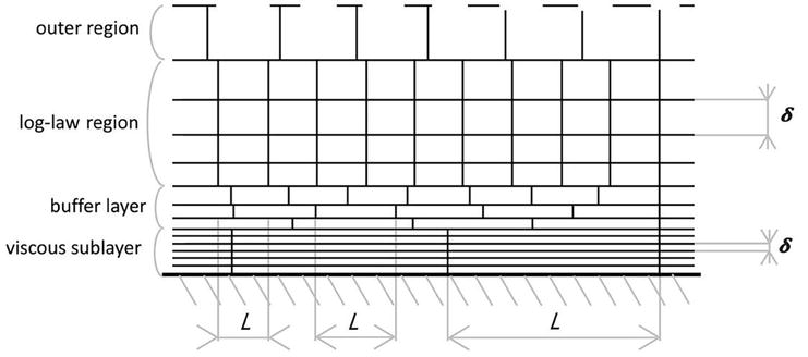
If converting this drastic idea of fractures into a Newtonian fluid, it is immediately realised that the corresponding concept to a solid fracture is that of a slip flow. In [23], it was argued that if this assumption is made on slip flow occurring in case a far-from-equilibrium irreversible process onsets, then with some basic mathematically and physically realistic assumptions on the connection between a local slip length and a local slip velocity to be directly proportional, i.e. $L=C_B{U}_{\text{slip}}$ (Figure 1).

Figure 1.

Fracture structure for a turbulent fluid flow parallel to a solid wall, resulting in fully developed viscous sublayer, buffer layer and log-law zones. Note that organisation of $L$ and $\delta$ totally depend on the experimentally recorded velocity vs. ${y_2}^{+}$ (except resolution). Locally, the flow has the same kinetic energy dissipation and same velocity gradient as long as the ratio of $L$ vs. $\delta$ is the same, cf. [23].

Instead of fractures originating from a bullet hole radially in a solid, consider the assumption for a turbulent wall-bounded flow, where instead square flakes originating from the wall, with slippage $U_{\text{slip}}$ in the $y_1$-direction, where the flake thickness is $\delta$, flake length is $L$ and flake width is $K$. One can then organise the $L$ and $\delta$ to reproduce the experimental viscous sublayer, buffer layer, and log-law regions (Figure 1).

The friction force of a single flake can be replaced by a shear stress acting on the flake, $\tau =F_1/A=F_1/\left(K·L\right)$, which gives a kinetic energy dissipation rate per unit volume $\mathrm{d}{\left(\mathrm{ke}\right)}_{\mathrm{res}}/\mathrm{d}t=\tau ·U_{\text{slip}}/\delta$ locally within the flow when ensemble averaging.

A second assumption is that $\tau \propto U_{\text{slip}}$. From this, one may postulate: $\tau =C_A·\rho ·C_B·U_{\text{slip}}$, which gives:

$$\frac{\mathrm{d}{\left(\mathrm{ke}\right)}_{\mathrm{res}}}{\mathrm{d}t}=C_A\frac{\mathit{\rho L}}{\delta }{U}_{\text{slip}}$$E1

Similarly to the case with the fractures in the bullet hole, the local kinetic energy dissipation is the highest in the viscous sublayer, where the slip length $L$ is the longest, together with the fracture thickness $\delta$ is the smallest. Immediately, with the present formulation, it is found that for fully developed turbulent pipe flows at ${Re}_D\ge 5000$, the net kinetic energy dissipation in the viscous sublayer is larger than the remaining net kinetic energy dissipation throughout all the other zones together. In addition, within the viscous sublayer zone, there is no eddy activity, at all.

The action of the far-from-equilibrium process along a viscous sublayer, can be illustrated with the example of an erosion rippling process [29], caused by an impacting jet stream of round hard particles impacting a ductile solid surface at a low angle of attack – described in detail in [23]: It is argued that a far-from-equilibrium slip-roll zone is built up closest to the wall. Two other zones can be identified, one zone with no far-from-equilibrium process occurring at all, which represents the major part of the entire flow volume. An intermediate zone also exists, which is a mixture of both the local zones of far-from-equilibrium processes being onset, as well as local offset zones. It has been identified that prior to the rippling process initiating, the reflecting flow is “laminar” [29], while when the rippling process has onset, the reflecting flow is “turbulent” [29]. Hence, for this case, the observation of a turbulent behaviour is a clear indication, or symptom, on the initiation of an erosion rippling process at the ductile wall surface [23].

2.3 Variation of shear stress across a turbulent boundary layer

By organising the time-averaged mean velocity variation in accordance with experiments as proposed in [23], and applying a novel fundamental model, a well-organised kinetic energy dissipation rate across the boundary layer appears to occur, cf. Figure 7 in [23]. Hence, the viscous sub-layer, buffer layer, and the log-law regions may seem to occur because of a self-organised grouping of fracture cells (to maximise the overall entropy production of the turbulent flow), cf. Section 2.6 in [23].

In this grouping, it becomes evident that the viscous sublayer represents a region of saturated – i.e. maximum entropy generation per unit volume, or equivalently, a maximum kinetic energy dissipation per unit volume. The significant amount of net kinetic energy dissipation within the viscous sublayer region, which may account for more than 50% of the total net kinetic energy dissipation of the total flow, immediately suggests that the specific thickness of the sublayer must have significant effect on the net kinetic energy dissipation, and that this thickness variation of the sublayer needs to be incorporated in the analysis [23].

Section 2.7 in [23] describes an approach in which the fracture model may account for the effects of various surface roughnesses, which is consistent with experimental observations on increasing of the ${U_1}^{+}$ intersection point of the log-law relation in the ${y_2}^{+}$ axis. (The Moody diagram also indicates an increased pressure drop [24] for situations when the surface roughness is higher.) A model is proposed, on how the $C_A$ and $L$ parameters vary with position from the wall, for different wall surface roughness conditions, cf. Section 2.7 in [23], and Figures 8–9 in [23]. This model can be simplified into a model describing the conditions in the viscous sublayer $C_A{L}_{\max }$, by which all other conditions throughout the turbulent wall boundary layer can be obtained in a non-dimensional manner, cf. Eqs. 17 and 18 in [23].

Also, with this novel fundamental model, it becomes immediately obvious why the generation of different zones – viscous sublayer, buffer region, log-law (or overlap) region, as well as the outer region of a turbulent boundary layer develops:

• Viscous sublayer: saturated region, constant $L=L_{\max }$ and constant $\delta$.

• Buffer region, varying $L$ and varying $\delta$. Transitional region between log-law and viscous sublayer, not saturated, hence defects may occur, resulting in visible swirls (visible/recordable eddies). Due to varying $L$ and $\delta$ as compared to neighbouring cells, a greater likelihood of creation of visible swirls (buffer region is identified as a “turbulence” (or visible eddy) production region).

• Log-law region: constant $L\approx L_{\max }/6$, but varying $\delta$. Not saturated, hence defects may occur, resulting in visible swirls (visible/recordable eddies)

• Outer region: a region with only occasional presence of onset novel fundamental zones. In the interface between novel fundamental zone and Newtons viscosity law zone, results in large swirly behaviour – which is understood as “large turbulent eddy” behaviour or “large-scale turbulence” by the external observer.

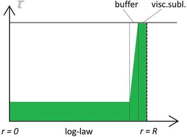
This organisation of fracture cells across a turbulent wall boundary layer, results in a corresponding principal shear stress variation (not to scale) for a fully developed turbulent pipe flow which can be depicted in Figure 2.

Figure 2.

Shear stress across a pipe cross-section according to novel approach, where $L=L_{\max }$ within the viscous sublayer is approximately 6 times larger than $L$ in the log-law region. Shear stress across all these regions is governed by the relation $\tau =\rho C_{A}L$. The action of the novel approach fundamental mechanism is coloured in green.

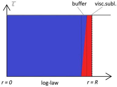
The corresponding principal shear stress variation (not to scale) for the CTT case at fully developed conditions is depicted in Figure 3, while shear stress for a laminar-flow case at fully developed conditions is depicted in Figure 4.

Figure 3.

Shear stress across a pipe cross-section according to CTT, where viscous processes (their action marked in red colour) account for 100% of shear stress within the viscous sublayer, and Reynolds stresses (their action marked in blue colour) account for 100% of shear stress within the log-law region. The buffer layer shear stress is a combination of these two shear stress mechanisms.

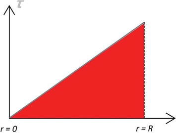
Figure 4.

Shear stress across a pipe cross-section for laminar flow (at fully developed laminar pipe-flow conditions), where the shear stress across all these regions is governed by the relation $\tau =-\mu \frac{\partial U_1}{\partial r}$. The fundamental mechanism based on Newton’s viscosity law describes the action of the viscous processes (their action marked in red colour) which account for 100% of shear stress within the entire pipe cross section.

The shear stress behaviour as computed by the novel approach across the viscous sublayer is constant but differ in magnitude as compared to CTT. This represents the main difference between CTT and the novel approach: The shear stress according to the novel approach is approximately 6 times higher than the shear stress computed for the log-law region.

From a modelling point of view, the parameter $C_{A}L$ takes the role of the Reynolds stress $-\overline{u_1{u}_2}$ within the log-law region, which according to CTT is constant throughout the low-law region. Note that $C_{A}L$ is according to the novel approach also constant throughout the log-law region, cf. Section 2.6 in [23]. The shear stress expressions (for pipe flows) in the various zones are summarized in Table 1.

Zone	Novel approach	CTT	Laminar flow
viscous sublayer	$\tau =\rho C_{A}L$; $\left(=\rho C_A{L}_{\max }\right)$	$\tau =-\mu \frac{\partial U_1}{\partial r}$	$\tau =-\mu \frac{\partial U_1}{\partial r}$
buffer layer	$\tau =\rho C_{A}L$	$\tau =$; $\text{part}\left(-\rho \overline{u_1{u}_2}\right)+\text{part}\left(-\mu \frac{\partial U_1}{\partial r}\right)$	$\tau =-\mu \frac{\partial U_1}{\partial r}$
log-law region	$\tau =\rho C_{A}L$	$\tau =-\rho \overline{u_1{u}_2}$	$\tau =-\mu \frac{\partial U_1}{\partial r}$
outer region	$\tau =$; $\text{part}\left(\rho C_{A}L\right)+\text{part}\left(-\mu \frac{\partial U_1}{\partial r}\right)$	$\tau \to 0$	$\tau =-\mu \frac{\partial U_1}{\partial r}$

Table 1.

Expressions for the variation of the shear stress in a laminar and a turbulent pipe flow. CTT assumes a constant shear stress, while the novel approach relies on a time-averaged mean velocity profile.

3. Flow modelling

3.1 Test case - fully-developed turbulent pipe flows

A computation of 20 different turbulent flow cases of fully developed pipe flows, for air flow at 20 °C in a 14 cm diameter tube, with different surface roughnesses, arrives at results according to Table 2.

$Re$	$f$	${\tau }_{\text{wall}}$ ($\mathrm{N}{\mathrm{m}}^{-2}$)	$\epsilon /D$	$U_{\text{mean}}$ ($\mathrm{m}{\mathrm{s}}^{-1}$)	$C_A{L}_{\max }$ (${\mathrm{m}}^2{\mathrm{s}}^{-2}$)	% of $\frac{\mathrm{d}\left(\mathrm{KE}\right)}{\mathrm{d}t}$ in v. subl.	% of $\frac{\mathrm{d}\left(\mathrm{KE}\right)}{\mathrm{d}t}$ in buffer r.	% of $\frac{\mathrm{d}\left(\mathrm{KE}\right)}{\mathrm{d}t}$ in log-law
5000	0.03739	0.001638	0	0.5393	0.002103	60.0	36.1	3.9
5000	0.03745	0.001641	0.00005	0.5393	0.002105	60.0	36.1	3.9
5000	0.03795	0.001663	0.0005	0.5393	0.002114	59.8	36.2	3.9
5000	0.04261	0.001867	0.005	0.5393	0.002178	58.2	37.9	3.9
5000	0.07595	0.003327	0.05	0.5393	0.002695	82.8	17.2	0.0
1 × 10^4	0.03088	0.005415	0	1.079	0.007380	58.2	35.9	5.9
1 × 10^4	0.03096	0.005429	0.00005	1.079	0.007386	58.2	35.9	5.9
1 × 10^4	0.03164	0.005549	0.0005	1.079	0.007445	58.0	36.0	6.0
1 × 10^4	0.03763	0.006599	0.005	1.079	0.008109	58.0	38.8	3.2
1 × 10^4	0.07380	0.01294	0.05	1.079	0.01052	82.6	17.4	0.0
1 × 10^5	0.01799	0.3155	0	10.79	0.5251	54.6	34.5	8.5
1 × 10^5	0.01826	0.3202	0.00005	10.79	0.5290	54.6	34.5	8.5
1 × 10^5	0.02033	0.3565	0.0005	10.79	0.5587	54.7	34.8	8.4
1 × 10^5	0.03131	0.5491	0.005	10.79	0.7179	56.6	38.6	4.8
1 × 10^5	0.07178	1.259	0.05	10.79	1.028	82.4	17.6	0.0
1 × 10^6	0.01165	20.43	0	107.9	41.39	53.6	33.9	8.7
1 × 10^6	0.01265	22.18	0.00005	107.9	43.14	53.6	34.0	8.7
1 × 10^6	0.01721	30.18	0.0005	107.9	50.66	54.0	34.4	8.7
1 × 10^6	0.03047	53.43	0.005	107.9	71.14	56.9	38.9	4.2
1 × 10^6	0.07157	125.5	0.05	107.9	102.5	82.4	17.6	0.0

Table 2.

Computations. The net integrated kinetic energy dissipation across a 1 m pipe, across the radius, using Eq. 18 in [23], arrives at a number multiplied by ${\mathrm{C}}_{\mathrm{A}}{\mathrm{L}}_{\max }$. This number is compared to the corresponding experiments computed using eq. 13 in [23]. The ${\mathrm{C}}_{\mathrm{A}}{\mathrm{L}}_{\max }$ coefficient is determined resulting in the net kinetic energy dissipation of the computations matching the corresponding experiments – i.e. a 1st law balance agreement between experiments and computations with novel approach model. Time-averaged mass flow rates in full agreement. Time-averaged velocity profile is in full agreement. (originally presented in [24]).

According to Table 2, the viscous sublayer and buffer regions contain most of the kinetic energy dissipation occurring. Most importantly, results with this novel approach arrives at a finding that the zones with turbulence generation and large eddies have a low, marginal, influence on the net kinetic energy dissipation.

In Section 3.4 in [24] a discussion is offered, on estimating the influence from visible eddies themselves, arriving at numbers as low as 1–3% influence caused by the visible eddies as compared to the overall flow. In present novel approach, it is zones with locally reduced kinetic energy dissipation which cannot maintain the onset of the novel fundamental slip flow, which results in imbalances of forces, which in turn may result in the onset of a swirling eddy. As discussed in Section 2.1, the presence of defect zones is a natural occurrence in a far-from-equilibrium large-scale ordered structuring, which is why swirls may occur. In contrast, also as stated in Section 2.1, any such “defect” zones cannot exist in a near-thermodynamic equilibrium irreversible continuum process governed by Newton’s viscosity law, hence swirls cannot be created in this way.

In Section 2.9 in [23], the analysis of turbulence onset is offered. A recent analysis of the onset/offset between laminar flows and the slip-fracture structure for fully developed pipe flows, arrived at onset/offset Re_D-numbers in fair agreement with corresponding experiments, i.e. around 2300 for the situation the wall surface roughness is smooth ($\epsilon /D=0.00$) and if assuming a slightly (50%) higher velocity gradient in the onset position (in the vicinity of the solid wall) in the laminar-flow side of the turbulent spot [3, 30, 31, 32, 33].

3.2 Flat plate developing boundary-layer flow

3.2.1 Traditional description of boundary layer flow along a flat plate

The literature describes a boundary layer flow along a flat plate, which initially is laminar, and at a critical position $x_{\mathrm{cr}}$, onsets a turbulent flow boundary layer. For both the laminar zone of the boundary layer, and the turbulent zone of the boundary layer, it has been experimentally found that the thickness of the boundary layer increases with downstream position $x$.

The literature presents various ways of analysing these flows. For the laminar flow zone without a pressure gradient along a plate, the Blasius relations (cf. Section 7.4 in [2]) allow the computation of the boundary layer thickness and wall shear stress – which varies along the downstream position $x$.

3.2.2 Applying the proposed theory of turbulence onset for a developing boundary-layer flow

Regarding the turbulence onset, and possibilities to estimate this, consider the original set of equations (Eqs. 20–21 in [23]), which described the local conditions for onset in a stationary pipe flow by equalling both the local kinetic energy dissipation for the two fundamental models, as well as simultaneously equalling the velocity gradient. Combining these two equations, and considering the velocity gradient in the vicinity of the solid wall, the condition for onset can be expressed as:

$${\left.C_A{L}_{\max }\right|}_{\text{onset}}=\nu {\left.\frac{{\partial U}_1}{{\partial y}_2}\right|}_{\text{onset}}$$E2

Noteworthy is that this relation only states the condition at the onset position along a solid wall.

Onset of turbulence in a fully developed pipe flow at stationary flow conditions:

For turbulence onset in a stationary pipe flow, the behaviour at steady-state stationary flows is recorded, across a certain section (which can be comparatively short), assuming the flow has fully developed. Hence, the possible distance from flow inlet to the section of testing, i.e., the distance required to reach fully developed flow conditions, could be hundreds of diameters in length, or more. The net flow rate is then adjusted, whereby a new steady-stationary flow is developed for this new flow rate condition. However, around a critical flow velocity, between the laminar flows and turbulent flows, if controlling the flow carefully, it is sometimes possible to arrange a flow allowing the observation of stationary turbulent spots building up along the wall at fixed positions. Also, one may ascertain their spreading around the circumference at a fixed downstream position, after which the turbulent flow is onset.

Onset of turbulence along a non-developed boundary layer:

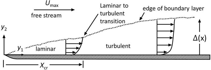
Consider a steady-state observation of Figure 5, which represents the relevant observation from the $z$ (or $y_3$) direction. Although the flow observed from the $z$ direction appears stationary, the flow should not be considered fully developed at any position along the plate, i.e., along the $x$-direction ($y_1$-direction), as the boundary-layer behaviour varies along the plate.

Figure 5.

Traditional description of a boundary layer flow developing at a flat plate, with onset of turbulence occurring at a critical position $x_{\mathrm{cr}}$. The thickness $∆$ of the boundary layer in turbulent state develops more rapidly than the laminar flow boundary layer thickness, with increasing downstream position $x$.

In the following example, it is assumed that the boundary layer along a flat plate develops also in a similar manner in a pipe flow with initial laminar inflow at the beginning of the pipe. Hence, an attempt is made to connect the onset for several different pipe flows, using Eq. 2.

3.2.3 Estimating ${\mathrm{C}}_{\mathrm{A}}{\mathrm{L}}_{\max }$ values at the turbulence onset condition from empirical observations

To verify the theoretical estimation Eq. 2 from the fracture-structure approach, an attempt is made to estimate the range of $C_A{L}_{\max }$ values corresponding to the Re_x numbers between $5\times {10}^5$ and $3\times {10}^6$, i.e., the empirically found range for turbulence onset.

From an empirical finding [24]¹, it is fair to assume the following at the onset position:

$$C_A{L}_{\max }\propto {\left(U_{\max }\right)}^2\text{or}{C}_A{L}_{\max }=\xi {\left(U_{\max }\right)}^2$$E3

At the onset position, assume that the velocity gradient in the vicinity of the wall is approximately:

$${\left.\frac{\partial U_1}{\partial y_2}\right|}_{\text{near wall}}\approx 10\frac{U_{\max }}{∆}$$E4

where $\mathrm{\Delta }$ is the local thickness of the boundary layer (at the onset position).

Introducing Eqs. 3 and 4 into Eq. 2 then gives the following relation at the onset position:

$$\frac{10x}{∆}\approx \xi {Re}_x$$E5

The boundary-layer thickness at the onset position can be estimated from the laminar-flow boundary layer thickness (Blasius formula), cf. [2]:

$$∆=\frac{5x}{\sqrt{{Re}_x}}$$E6

Combining Eqs. 5 and 6 gives at the onset position:

$$\xi =\frac{2}{\sqrt{{Re}_x}}$$E7

which for onsets at ${Re}_x$ numbers between $5\times {10}^5$ and $3\times {10}^6$ corresponds to onsets at $\xi$ numbers between 0.0011547 and 0.0028284. In turn, the corresponding range of ${\left.C_A{L}_{\max }\right|}_{\text{onset}}$ for various pipe flows can be estimated using Eq. 3.

First iteration:

Is it possible to directly estimate the ${\left.C_A{L}_{\max }\right|}_{\text{onset}}$ at the onset position, and to compare this with the range of ${\left.C_A{L}_{\max }\right|}_{\text{onset}}$ computed from the range of ${Re}_x$ numbers at which turbulence is considered to onset?

Without information on variations along the boundary layer, one important parameter that may be useful is the concept of friction velocity – originally defined as a scaling velocity for a turbulent boundary layer. This concept can be extended in the following, as it is in the traditional turbulence sciences stated to not represent any real velocity. However, for the fracture structure model, the friction velocity can be demonstrated to equal the slip velocity in the viscous sublayer, for a situation where the fractures are assumed to separate 1 turbulence wall units from each other in the $y_2$ direction. This observation directly follows from the relation $U^{+}\approx y^{+}$ in the viscous sublayer^.2.

If, in the first iteration, it is assumed that the friction velocity at the onset position equals the friction velocity of a corresponding fully developed turbulent pipe flow, then Eq. 2 for onset can be rephrased into:

$${\left.C_A{L}_{\max }\right|}_{\text{onset}}={\left(U^{\ast }\right)}^2$$E8

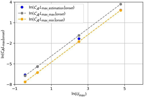
For the pipe flow turbulence onset estimations (assuming $\epsilon /D=0$), we obtain Table 3 in the first iteration. Plotting the natural logarithm of the $U_{\max }$ on the $x$-axis, and the natural logarithms of ${\left.C_A{L}_{\max }\right|}_{\text{onset}}$ on the $y$-axis, gives Figure 6.

${Re}_D$	$U_{\max }$	$U^{\ast }$	${\left.\frac{\partial U_1}{\partial y_2}\right|}_{\text{near wall}}$ Eq. 4	${\left.C_A{L}_{\max }\right|}_{\text{onset}}$; Eq. 2	${\left.C_A{L}_{\max }\right|}_{\text{onset}}$ (${Re}_x=5\times {10}^5$) Eq. 3	${\left.C_A{L}_{\max }\right|}_{\text{onset}}$ (${Re}_x=3\times {10}^6$) Eq. 3
$5\times {10}^3$	0.64667	0.0368692	90.0223	0.001359	0.000483	0.001183
$1\times {10}^4$	1.27352	0.0670356	297.6009	0.00449	0.001873	0.004587
$1\times {10}^5$	12.2575	0.511689	17339.5	0.2618	0.1735	0.4250
$1\times {10}^6$	119.578	4.11757	1,122,520	16.95	16.51	40.44

Table 3.

Estimating onset position for 14 cm diameter pipe flows, with air flowing at 20°C (first iteration). Data of fully developed pipe flows were taken from [24]. The Centre-line velocity ${\mathrm{U}}_{\max }$ estimated from the log-law relation for smoothness factor 0.0.

Figure 6.

Graph of $ln\left({\left.C_A{L}_{\max }\right|}_{\text{onset}}\right)$ vs. $ln\left(U_{\max }\right)$ for computations of the onset position in the first iteration, according to example case results presented in Table 3.

The empirical ${\left.C_A{L}_{\max }\right|}_{\text{onset}}$ numbers occur within the zone between grey dots and orange dots (which corresponds to the ${Re}_x$ interval between $5\times {10}^5$ and $3\times {10}^6$). The blue dots represent the estimated ${\left.C_A{L}_{\max }\right|}_{\text{onset}}$ calculation from Eq. 8, if assuming the friction velocity in the onset position equals the friction velocity of a corresponding fully-developed turbulent pipe flow – which for three of the four cases fall within the onset zone.

Second iteration:

It should again be stressed that the ${\left.C_A{L}_{\max }\right|}_{\text{onset}}$ estimated in Table 3 (first iteration), represents the condition in the turbulence onset position, and nowhere else. To illustrate, the $C_A{L}_{\max }$ for the corresponding fully developed pipe flow conditions along solid walls at stationary turbulent flow are different than in Table 3. According to Table 1 in [24], the corresponding values are $C_A{L}_{\max }$ = 0.002103 at ${Re}_D=5\times {10}^3$, $C_A{L}_{\max }$ = 0.007380 at ${Re}_D=1\times {10}^4$, $C_A{L}_{\max }$ = 0.5251 at ${Re}_D=1\times {10}^5$, and $C_A{L}_{\max }$ = 41.39 at ${Re}_D=1\times {10}^6$.

The onset estimation may be improved, by refining the estimations on ${\left.C_A{L}_{\max }\right|}_{\text{onset}}$ and the velocity gradient.

For instance, if the velocity gradient where onset occurs is 50% lower, then it should be noted that adjusting Eq. 4 into ${\left.\frac{\partial U_1}{\partial y_2}\right|}_{\text{near wall}}\approx 5\frac{U_{\max }}{∆}$, and consequentially adjusting Eqs. 5–7, then a recalculation will result in the following changes in Table 3 and Figure 6: The numbers in the four rightmost columns of Table 3 will be 50% lower, and Figure 6 would appear similar, but with a factor 2 difference in plotting all y-axis numbers.

In conclusion, the analysis in Sections 3.2.2–3.2.3 indicates that – despite exact numerical values on flow gradient at the onset position are not known – there appears to exist a single onset position $x_{\mathrm{cr}}$ in a developing boundary layer flow.

Also, in terms of $C_A{L}_{\max }$ numbers, for the guess made in the first iteration arrived at onset of turbulence occurring prior to reaching fully developed turbulent flow conditions in the pipe, which is a necessary result. Also, looking at the $C_A{L}_{\max }$ numbers for the ranges of ${Re}_x$-numbers, all intervals occur prior to the pipe-flow turbulence reaching fully developed flow conditions.

It is not clear, however, if the predicted $C_A{L}_{\max }$ value at onset for the case ${Re}_D=1\times {10}^6$ is too high, as these numbers are rather close to the $C_A{L}_{\max }$ at fully developed turbulent conditions, according to data from [24]. A scaling as demonstrated in the second iteration, may be required to adjust the $C_A{L}_{\max }$ values, when more data becomes available.

3.3 Analysis with classical turbulence theory - failure to predict onset

According to CTT, the viscous sublayer is considered a thin layer where no eddies are present. The irreversible processes assumed in CTT are the near-equilibrium continuum irreversible process of viscous shear flow, resulting in viscous dissipation.

At the onset point, in the vicinity of the solid wall, assuming the flow gradient on the laminar flow side to be ${\left(\partial U_1/\partial y_2\right)}_{\text{laminar}}$, at the turbulence side, the flow gradient is ${\left(\partial U_1/\partial y_2\right)}_{\text{turbulent}}$.

The total kinetic energy dissipation equals the viscous dissipation, which for the laminar flow case can be expressed as $\frac{\mathrm{d}{\left(\mathrm{ke}\right)}_{\text{viscous}}}{\mathrm{d}t}=\mu {\left.{\left(\frac{\partial U_1}{\partial y_2}\right)}^2\right|}_{\text{laminar}}$. For the turbulent case, a corresponding expression can be derived.

For a fully developed pipe flow situation, according to CTT, for the same mean flow rate, the friction factor according to the Moody diagram for corresponding fully developed pipe flows is 60–180% larger (depending on wall surface roughness) for the turbulent flows at Re_D = 2300, as compared to the friction factor for laminar flow. There seems to be no overlap of the friction factors in the transitional region within the Moody diagram with the laminar flow friction factor.

Hence, according to Eq. 10 and 12 in [23], the wall shear stress is for the same mean flow rate, will always be different for the turbulent flow case compared to the corresponding laminar flow case, which is also the case at the onset point. Hence, according to CTT, the flow gradient at the wall – directly connected with the wall shear stress – will always be different at all hypothetical onset points, when comparing the flow gradients at the same wall position for situation of turbulent flow or corresponding laminar flow at the same mean flow rate. The same is also the case for kinetic energy dissipation in the vicinity of the wall. Hence, it is not possible to find any common geometrical position according to CTT where the flow gradients are equal for both laminar flow case and turbulence flow case, and simultaneously the local kinetic energy dissipation is equal for both the laminar flow case and corresponding turbulent flow case.

Hence, it is not possible to use the CTT to analytically predict the turbulence onset.

4. Considerations for near-wall flow measurements and simulations

4.1 Cascade theory and 1st law of thermodynamics: Suggesting a low influence of visible eddies on net kinetic energy dissipation

If relevant processes are better understood, this may prove beneficial when considering apparatus design.

Consider, e.g., the Cascade theory of Richardson [34] and Kolmogorov [35] and the 1st law of thermodynamics. While so-called “energy budgets” of visible eddies have been presented in CTT literature, however, no obvious connection to the 1st law of thermodynamics has been presented. Hence, is it possible to make a 1st law analysis of the turbulent flow incorporating the cascade theory?

Yes, this may be possible. The results obtained in [24], indicated that the net contribution of the outer layer to the total kinetic energy dissipation was somewhere between 0 and 3.8% (of the total kinetic energy dissipation of the flow) for all cases studied. The net contribution of the log-law region to the total kinetic energy dissipation was somewhere 0–8.7% (of the total kinetic energy dissipation of the flow) for all cases studied. More importantly, the contribution of the kinetic energy dissipation as caused by the visible eddies in these regions appears to be less than these numbers. In Chapter 3.4 in [24] it was argued that the presence of visible eddies connected to the presence of defect zones, i.e. a local zone with reduced influx of work to be consumed by the irreversible process, as these defects could generate the visible eddies. The net effect on the total kinetic energy dissipation in the pipe flow – due to the actions (direct and indirect) of all visible turbulent eddies – was estimated to be within the range of 1–3% (reduced net kinetic energy dissipation) of the net total kinetic energy dissipation of the turbulent flow, cf. estimations in Section 3.4 in [24].

The following arguments can be made that the findings in [24] are in line with the Cascade theory:

• First, the original cascade theory does not state which fundamental model is valid during the cascading of eddies. Only the last step, the conversion of the smallest eddies into viscous dissipation, occurs via Newtons fundamental model. (There is no contradiction here, as stated in [23, 24], for the smaller flow gradients, the maximum entropy generation will occur for the Newtons viscous irreversible process, hence within the outer layer, the eddies dying out will eventually reach small gradients, and be converted into viscous dissipation).

• Second, the original cascade theory, in itself, will suggest the net amount of viscous dissipation is caused by the turbulent eddies in a turbulent pipe flow: A 1st law analysis, if strictly following the assumption that larger scale eddies may transform – without any direct or indirect energy interaction with the main time-averaged flow – into smaller-scaled eddies with preserved kinetic energy, this assumption has major implications: The 1st law analysis, due to the downstream translation invariance for a fully developed pipe flow, will show that the work input (or work “injection” as referred to in the Cascade Theory) required to generate the largest-scale eddies is approximately 1–3% of the net kinetic energy of the kinetic energy of the time-averaged flow, obtained from the relation ${\left(\text{kinetic energy}\right)}_{\text{largest scales}}=\frac{1}{2}\left({\left({u_1}^{\prime }\right)}^2+{\left({u_2}^{\prime }\right)}^2+{\left({u_3}^{\prime }\right)}^2\right)$ (in units J/kg) which is approximately 1–3% of the kinetic energy of the time-averaged flow (the fluctuating component ${u_1}^{\prime }$ is the largest fluctuating component in a pipe flow with mean flow in the $y_1$-direction, approximately 10% of U_mean, while the other two fluctuating components are much smaller). Hence, since no kinetic energy dissipation or viscous dissipation is assumed to occur in the cascading process, and no kinetic energy is transferred from the mean flow to the smaller-scale eddies, it is a physical necessity that the last step which converts kinetic energy into viscous dissipation represents the same 1–3% of the net input kinetic energy, i.e. the net contribution of all visible/cascading eddies to the dissipation of total turbulent flow is only some 1–3%. (We keep in mind that work input in the form of maintaining a steady work input per unit time, while dissipation occurs across a certain volume – which is why units for kinetic energy of time-averaged flow and largest eddies differ from the units of dissipation, while the specific percentage number range 1–3% remains the same. This same 1–3% influence of the defect zones (generated by visible eddies) of the total kinetic energy dissipation of the total flow was also obtained in the results estimated in [24]. (Most important to note: While cascade theory correctly describes 100% of the viscous dissipation to be caused by the turbulent eddies at the smallest Kolmogorov scales, it does nowhere claim this viscous dissipation to represent the 100% kinetic energy dissipation of the entire turbulent flow).

4.2 Planning experiments within viscous sublayer and buffer region

If designing experiments on turbulent boundary-layer flows, the insights gained by the novel approach (if the experimentalist would wish to consider the behaviour predicted in this paper, and in [23, 24]), the following recommendations are made:

• Consider zones of high net kinetic energy dissipation as more important to experimentally analyse, as compared to low-kinetic energy dissipation zones. For instance, the viscous sublayer has the highest kinetic energy dissipation, and is for this reason the zone where turbulence onset triggers.

• Consider experimental mean velocity flow meters based on the Hot-Wire technique as dependable, except in the vicinity of a solid wall (where heat losses to the wall may disturb the measurement). The mean flow profile, after non-dimensional scaling, can be connected to $L$ and $\delta$ in various zones across the boundary layer.

• Be aware of the potential differences in onset/triggering behaviour, where the presence of a nano-scale particle may appear to have negligible disturbance within a continuum viscous process flow gradient, while, in contrast, may very well result in unexpected behaviour within a far-from-equilibrium process condition. (A surface holographic interference analysis apparatus was developed by [36], however they failed to obtain spatial resolution when testing within a viscous sublayer, for reasons unknown [37]). Most turbulence scientists, for instance, are familiar with the ease at which a natural-convection smoke fume from a stationary cigarette at ambient indoor conditions onsets into turbulence. The following question should be posed: Does the smoke particles contribute to the onset of turbulence in this case?

• To allow basic analysis with the novel approach, initial data extracted from a Moody diagram or corresponding Colebrook equation can be used, for analysis in pipe flows. For instance, all computations in [23, 24] utilised the Colebrook equation, and the results from [24] was also applied in this paper, to estimate onset condition along a developing-boundary layer flow along a solid wall. The experimental tools originally used to create the Moody diagram (where Colebrook equation is a mathematical formula providing Moody data within 1.5% accuracy) where recorders of pressure drop, recording devices for the mean flow rate, as well as a scale for the representation of the wall surface roughness, expressed in dimensionless form relative roughness $\epsilon /D$. Also, experimental tools to record the viscosity of the Newtonian fluid is necessary, to compute the relevant Reynolds number. The Moody chart was obtained with data obtained at or around ambient temperatures.

• To consider experiments for model improvements, one approach is to consider better understanding of $L_{\max }$ and $\delta$ within the viscous sublayer. Visualisation techniques and the introduction of dye or gas bubbles could be made within the viscous sublayer, to estimate the nature and size scales of $L_{\max }$ and $\delta$. Some near-wall visualisation techniques may be used, for this purpose. Through dye injection or injection of hydrogen bubbles (by electrolysis), one has with high-speed video motion photography observed phenomena such as “burst-sweep cycles,” which include the description of motion of “ribbon-like” patterns of fluid within the viscous sublayer, resulting in the variation of the thickness of the viscous sublayer with time. In [23, 24], a discussion on the “overproduction” of “flakes” describes the release of far-from-equilibrium zones which release and flow downstream (moving downstream with a significantly lower speed, as compared to the local speed of the fluid flow itself).

• In [23, 24], a discussion on the shape of these flakes, which have a width $K$ and length $L$ (as the streaks align with the flow), which might connect with the length of the low-speed streaks (note that the flakes themselves may be moving with low speed or being stationary). The upwards movement experimentally found in these streaks is due to downward flow in high-speed areas (to fulfil the conservation of mass principle).

• In experiments, it has been found that the streaks shift inconsistently, and appear and disappear over time. In connection with the proposed novel approach, this could suggest that the flakes are occasionally not in contact with each other in the transverse-direction ($y_3$-direction) of the fluid flow direction ($y_1$-direction). The widths between these streaks suggest $K\approx 100+$ (turbulence wall units), while the length of these streaks suggest $L\approx 1000+$ (turbulence wall units) in length. (The Re numbers do not influence these numbers.)

• When studying the streaks, it is found that similar traces of streaks may be found up through the buffer- and log-law regions, maintaining the same width between the streaks, but with reduced length [38] – also in excellent agreement with novel approach. However, due to the visible eddy mixing, the presence of streaks weakens when moving further away from the wall.

• However, for the study of the effects of mixing, or downstream development of a turbulent wall-bounded flow boundary-layer thickness, the understanding of the rotation of the visible eddies do play an important role. This is particularly important for the study of e.g. heat transfer behaviour.

• One should not rule out the possibility of recording sound waves generated from the turbulent flow, to perform an analysis. In some reports [39], sound energy maxima are recorded at specific frequencies [39]. Is there any possibility to connect such maximums to the novel approach theory?

4.3 Planning of more detailed simulations accounting for an overall active far-from-equilibrium mechanism

It was estimated in [24] and in Section 4.1 that ignoring the transient simulation of swirls and eddies resulted in errors in kinetic energy dissipation of around 1–3%. The results of the steady-state simulations appear accurate enough to allow the computations of turbulence onset for fully-developed pipe flows, as well as for a developing-flow boundary layers – as presented in Section 3.

However, it should be mentioned that some aspects of a more detailed simulation or modelling – if one would wish to simulate various details of the near-wall flow behaviour – is possible, however, a bit more complex as compared to the complexity in existing CFD flow solvers. (A multiphase CFD flow solver may need to be used.) This aspect touches on the drawbacks with the novel approach: Consider, for instance, how to simulate the individual near-wall fracture cells. These may be active and be located at stationary positions. But these may also suddenly start to act in a non-stationary manner, by moving downstream. To further complicate the picture, if these cells move downstream, they will move at a much lower velocity as compared to the speed of a local fluid element.

It is important to distinguish the fracture cells behaviour from the fluid flow behaviour. If assuming that the behaviour of the fracture cells is controlled by an overall MEP process behaviour – which admittedly is not accurately known – provide formidable challenges for a simulation. Also, the movement of defects within the flow (directly impacting the vorticity or visible eddy behaviour), or if these are stationary or not (for instance, more stationary within the buffer region, while separated saturated zones are moving as small “islands” along the flow within the outer region of a turbulent boundary layer) are not well known.

Admittedly, existing far-from-equilibrium theory may not yet give accurate answers to all questions raised, but possibly provide some guidance on the turbulent flow behaviour, which connects to more complex modelling issues such as typical anisotropic behaviour of visible eddies [32] and memory effects [40] (or “coherence” in the turbulent fluid flow), as well as e.g. near-wall sweep-burst behaviour (cf. discussion of leakage of Residual-Thermodynamic Process zones in viscous sublayer, cf. [23, 24]), and approximately explain the location and behaviour of near-wall turbulent streaks, the size of these, the spacing of these, and why they occasionally vanish.

On a positive note, however, this “unknown behaviour” of MEP could be investigated in numerical simulations by – for instance – testing various injections of defects or defect clouds into various positions in the flows and observing the outcome. If a CFD flow solver is designed to be capable of simulating fracture cell movements and allowing for the simulation of visible eddies by injection of defect or defect clouds, then this may provide a great opportunity to investigate what type of MEP input would give a truly realistic turbulence simulation behaviour output. In this way, the observation of the above-mentioned various experimental phenomena near walls in the different near-wall zones, may become possible to simulate. For instance, phenomena such as apparent turbulent intensities (2nd-order statistics) in the flow may be simulated and evaluated.

5. Discussion and conclusions

A proposed novel approach on the modelling of turbulent flows, offers possibilities of additional understanding on several aspects of turbulent flows.

On the question of how the mechanism of onset of turbulence works; A discussion is presented, arguing for the comparison of flow conditions at a hypothetical onset point in the vicinity of a wall. By applying the novel approach model for the turbulence modelling, the onset Re numbers for fully developed pipe flows (computed in [24]) and the onset Re numbers for a developing-flow boundary layer along a wall can be computed. The onset estimations arrive at excellent agreement between modelling results and corresponding experiments. By applying the CTT approach, it is here demonstrated as well that no onset Reynolds numbers can be computed.

On the question of benefits obtained with the proposed novel approach, one may argue for a good connection of the novel approach with the original boundary-layer theory introduced by Prandtl, with possibilities to apply original dimensionless scaling concepts such as $U^{+}$, $U^{\ast }$ and turbulent wall dimension units. The parameter $C_A{L}_{\max }$, which can be extracted by model-fitting a couple of points in a Moody-diagram, provides an exponential correlation between $C_A{L}_{\max }$ and $U_{\text{mean}}$ (for data extracted at a specific wall surface roughness $\epsilon /D$), for all Reynolds numbers, cf. Eqs. 1 and 2 in [24], a correlation which also works when extrapolating far outside the points used for model-fitting, into a Reynolds numbers region where onset analysis can be successfully applied. (Hence, it is not required to fit model coefficients at actual onset flow conditions to predict onset.) One should also note that the novel approach draw attention to the problem of turbulence in an unprejudiced manner, with the core aim of analysing the large-scale behaviour with as few assumptions and simplifying assumptions as possible. While the specific assumptions and simplifying assumptions made for CTT can be criticised, it is also in this context worthwhile to mention the criticism presented in [41]: “So confident was the turbulence community in its beliefs that virtually no one even bothered to measure the skin friction, and it was simply inferred from fitting the log profile to a few points near the wall, usually for values of y+ between 30 and 100. In fact the ‘log’-based ideas were so well-accepted that it seemed to bother only a few that real shear stress measurements (both momentum integral and direct) differed consistently and repeatably from these inferred results.” The results presented in Figure 2 may explain the reasons for consistent and repeatable erratic prediction of the real wall shear stress.

Acknowledgments

Hot Disk AB (Sweden) supported this work. Special thanks to Prof. L. Löfdahl at Dept. of Mechanics and Maritime Sciences, Chalmers Univ. of Technology, D.Sc. S.E. Gustafsson at Dept. Physics, Chalmers Univ. of Technology and Dr. H. Otterberg at University of Gothenburg. Also, thanks to Dr. B. Mihiretie, Mr. A. Sizov and Ms. B. Lee at Hot Disk AB (Sweden), for assistance in preparing this manuscript.

Conflict of interest

The author declares no conflict of interest.

Nomenclature

A	area (${\mathrm{m}}^2$)
$C_A$	model constant ($\mathrm{m}{\mathrm{s}}^{-2}$)
$C_B$	model constant ($\mathrm{s}$)
$D$	diameter of pipe interior (m)
$\frac{\mathrm{d}{\left(\mathrm{ke}\right)}_{\mathrm{res}}}{\mathrm{d}t}$	kinetic energy dissipation rate per unit volume, due to residual process ($\mathrm{W}{\mathrm{m}}^{-3}$)
$\frac{\mathrm{d}{\left(\mathrm{ke}\right)}_{\text{viscous}}}{\mathrm{d}t}$	viscous dissipation rate for viscous laminar flows of Newtonian fluids per unit volume ($\mathrm{W}{\mathrm{m}}^{-3}$)
$F$	force ($\mathrm{N}$)
K	flake width (in $y_3$-direction) (m)
$L$	slip length of flake (in $y_1$-direction), cf. [23] ($\mathrm{m}$)
$R$	radius of pipe interior (m)
$Re$	Reynolds number (−)
$S$	entropy ($\mathrm{J}{\mathrm{K}}^{-1}$)
$U$	Velocity ($\mathrm{m}{\mathrm{s}}^{-1}$)
$u^{\prime }$	Fluctuating velocity (after Reynolds decomposition) ($\mathrm{m}{\mathrm{s}}^{-1}$)
$U^{\ast }$	Friction velocity ($\mathrm{m}{\mathrm{s}}^{-1}$)
Uslip	slip velocity ($\mathrm{m}{\mathrm{s}}^{-1}$)
$x$	distance from front edge of plate ($\mathrm{m}$)
$\mathrm{X}$	extensive thermodynamic flow
$y$	vertical distance (from the plate surface) ($\mathrm{m}$)
$z$	longitudinal-direction distance (from a hypothetical reference point or line, e.g., centreline of plate) ($\mathrm{m}$).
$y_1$, $y_2$, $y_3$	Cartesian co-ordinates ($\mathrm{m}$)

Greek letters

$∆$	boundary layer thickness ($\mathrm{m}$)
$\delta$	gap width between slip layers, also referred to as thickness of flake fracture, or resolution parameter ($\mathrm{m}$)
$\epsilon$	surface roughness ($\mathrm{m}$)
$\mu$	dynamic viscosity of the Newtonian fluid ($\mathrm{kg}{\mathrm{m}}^{-1}{\mathrm{s}}^{-1}$)
$\nu$	kinematic viscosity of the Newtonian fluid (${\mathrm{m}}^2{\mathrm{s}}^{-1}$)
$\xi$	model constant, introduced in Eq. (3) (−)
$\rho$	density ($\mathrm{kg}{\mathrm{m}}^{-3}$)
$-\rho \overline{u_1{u}_2}$	Reynolds stress ($\mathrm{N}{\mathrm{m}}^{-2}$)
$\tau$	shear stress ($\mathrm{N}{\mathrm{m}}^{-2}$)

Subscripts

$\mathrm{cr}$	(critical)
$D$	inner diameter-based
$max$	(maximum)
$\text{mean}$	(average)
$\text{near wall}$	vicinity of wall
$\text{onset}$	condition at the onset position
$\mathrm{res}$	for residual sub-process
$x$	flat plate-direction

Special notations

${\left(·\right)}^{+}$	dimensionless scaling (traditional), cf. Figure 2 in [24]
$\mathrm{d}\left(·\right)$	differential [e.g., ${\mathrm{d}}_{\mathrm{i}}{\mathrm{S}}_{\mathrm{res}}$ represents the differential entropy change due to residual process ($\mathrm{J}$${\mathrm{K}}^{-1}$)]

References

1.Phillips L. Turbulence, the Oldest Unsolved Problem in Physics. 2018. Available online: https://arstechnica.com/science/2018/10/turbulence-the-oldest-unsolved-problem-in-physics/
3.Panton RL. Incompressible Flow. 4th ed. New York, USA: John Wiley & Sons; 1984
4.Tritton DJ. Physical Fluid Dynamics. 2nd ed. New York, USA: Oxford University Press; 1988. p. 519
5.Tennekes H, Lumley JL. A First Course in Turbulence. Cambridge, Massachusetts, USA, and London, England: MIT Press; 1972
6.Davidson PA. Turbulence: An Introduction for Scientists and Engineers. New York, USA: Oxford University Press; 2004
7.Davidson PA, Kaneda Y, Moffatt K, Sreenivasan KR, editors. A Voyage through Turbulence. Cambridge, UK: Cambridge University Press; 2011
8.Monin AS, Yaglom AM. Statistical Fluid Mechanics. Vol. 1. Cambridge, MA: MIT Press; 1971. p. 769
9.Robinson SK. Coherent motions in the turbulent boundary layer. Annual Review of Fluid Mechanics. 1991;23:601-639
10.Smith CR. Coherent flow structures in smooth-wall turbulent boundary layers: Facts, mechanisms and speculation. In: Ashworth PJ, Bennett SJ, Best JL, McLelland SJ, editors. Coherent Flow Structures in Open Channels. Chichester, UK: Wiley; 1996. pp. 1-39
11.Corino ER, Brodkey RS. A visual investigation of the wall region in turbulent flow. Journal of Fluid Mechanics. 1969;37:1-30
12.Offen GR, Kline SJ. Combined dye-streak and hydrogen-bubble visual observations of a turbulent boundary layer. Journal of Fluid Mechanics. 1974;62:223-239
13.Offen GR, Kline SJ. A proposed model of the bursting process in turbulent boundary layers. Journal of Fluid Mechanics. 1975;70:209-228
14.Harun Z, Lofty ER. Generation, Evolution, and Characterization of Turbulence Coherent Structures. London, UK: IntechOpen; 2018. DOI: 10.5772/intechopen.76854
15.Demirel Y. Nonequilibrium Thermodynamics: Transport and Rate Processes in Physical, Chemical and Biological Systems. 3rd ed. Amsterdam, The Netherlands: Elsevier; 2014
16.Herrmann B, Oswald P, Semaan R, Brunton SL. Modeling synchronization in forced turbulent oscillator flows. Communications on Physics. 2020;3:195. DOI: 10.1038/s42005-020-00466-3
17.Moin P, Mahesh K. Direct numerical simulation: A tool in turbulence research. Annual review of fluid mechanics. 1998;30:539-578. DOI: 10.1146/annurev.fluid.30.1.539
18.Liu C, Lu P, Chen L, Yan Y. New Theories on Boundary Layer Transition and Turbulence Formation. Modelling and Simulation in Engineering. Cairo, Egypt: Hindawi Publishing Corporation; 2012; Article ID 619419. DOI: 10.1155/2012/619419
19.Bose R, Durbin PA. Transition to turbulence by interaction of free-stream and discrete mode perturbations. Physics of fluids. 2016;28:114105. DOI: 10.1063/1.4966978
20.Ducros F, Comte P, Lesieur M. Large-eddy simulation of transition to turbulence in a boundary layer developing spatially over a flat plate. Journal of fluid mechanics. 1996;326:1-36. DOI: 10.1017/S0022112096008221
21.Launder BE, Spalding DB. The numerical computation of turbulent flows. Computer methods in applied mechanics and engineering. 1974;3:269-289. DOI: 10.1016/0045-7825(74)90029-2
22.Hinze JO. Turbulence – An Introduction to its Mechanism and Theory. U.S.A.: McGraw-Hill; 1959
23.Gustavsson M. A residual thermodynamic analysis of turbulence – Part 1: Theory. International Journal of Thermodynamics. 2022;25:50-62. DOI: 10.5541/ijot.1017342
24.Gustavsson M. A residual thermodynamic analysis of turbulence – Part 2: Pipe flow computations and further development of theory. International Journal of Thermodynamics. 2022;25:64-75. DOI: oi.org/10.5541/ijot.1017374
25.Jaeger HM, Liu AJ. Far-from-equilibrium physics: An overview. arXiv. 2010. p. 1-23. DOI: 10.48550/arXiv.1009.4874. Eprint arXiv:1009.4874; EPub date: September 2010
26.Kondepudi D, Prigogine I. Modern Thermodynamics: From Heat Engines to Dissipative Structures. Chichester, UK: Wiley; 1998
27.Gustavsson M. Residual thermodynamics: A framework for analysis of non-linear irreversible processes. International Journal of Thermodynamics. 2012;15:69-82. DOI: 10.5541/ijot.346
28.Kleidon A, Malhi Y, Cox PM. Maximum entropy production in environmental and ecological systems. Philosophical Transactions of the Royal Society B. 2010;365:1297-1302. DOI: 10.1098/rstb.2010.0018
29.Finnie I, Kabil YH. On the formation of surface ripples during erosion. Wear. 1965;8:60-69. DOI: 10.1016/0043-1648(65)90251-6
30.Emmons HW. The laminar-turbulent transition in a boundary layer – Part I. J. Aero. Sci. 1951;18:490-498. DOI: 10.2514/8.2010
31.Emmons HW, Bryson AE. The laminar-turbulent transition in a boundary layer (part II). In: Proceedings of the first U.S. National Congress of Applied Mechanics (June 1951, Chicago, Illinois) A.S.M.E., 1952. pp. 859-868
32.Davis SH, Lumley JL. Frontiers in Fluid Mechanics. A Collection of Research Papers Written in Commemoration of the 65th Birthday of Stanley Corrsin. Berlin Heidelberg, Germany: Springer Verlag; 1985
33.Jonáš P. On the turbulent spot and calmed region. In: Proceeding of Engineering Mechanics 2007, National Conference with International Participation. Prague, Czech Republic: Institute of Thermomechanics, Academy of Sciences of the Czech Republic; May 14-17, 2007
34.Richardson LF. Weather Prediction by Numerical Processes. Boston: Cambridge University Press; 1922. p. 66 (ISBN 9780511618291.)
35.Kolmogorov AN. Local structure of turbulence in an incompressible fluid at very high Reynolds numbers. Doklady Akademii Nauk SSSR. 1941;31:99-101
36.Abrantes JK. Holographic Particle Image Velocimetry for Wall Turbulence Measurements, Ph.D. thesis,. Lille, France: Ecole Centrale de Lille; 2012
37.Abrantes JK. Private communication. 2023
38.Wang W, Pan C, Wang J. Wall-normal variation of spanwise streak spacing in turbulent boundary layer with low-to-moderate Reynolds number. Entropy. 2019;21:24
39.Succi GP. The Interaction of Sound with Turbulent Flow, Gas Turbine & Plasma Dynamics Laboratory Report no. 140. Cambridge, MA, U.S.A.: MIT; 1977
40.Ross D, Robertson JM. Shear stress in a turbulent boundary layer. Journal of Applied Physics. 1950;21:557-561. DOI: 10.1063/1.1699706
41.George WK. Recent advancements toward the understanding of turbulent boundary layers. In: Proceedings of the American Institute of Aeronautics and Astronautics. Reston VA, USA: American Institute of Aeronautics and Astronautics; 2005-4669
Notes
In [24], a connection was established as CALmax proportional to Umean1.87 at fully developed pipe flow conditions, when ε/D=0. (The power of 1.87 increased with increasing surface roughness, up to 1.99 for ε/D=0.05, for reasons discussed in Section 3.5 in [24]).
Note that enough resolution is required to apply the fracture structure model. In all computations in [23, 24], the resolution in the y-direction in the viscous sublayer was selected to be 1 turbulence wall unit.
Written By
Mattias K. Gustavsson
Submitted: 25 September 2023Reviewed: 29 October 2023Published: 13 February 2024