Solar Radiation Prediction Using an Improved Adaptive Neuro-Fuzzy Inference System (ANFIS) Optimization Ensemble

Abstract

A dependable design and monitoring of solar energy-based systems necessitates precise data on available solar radiation. However, measuring solar radiation is challenging due to the expensive equipment required for measurement, along with the costs of calibration and maintenance, especially in developing countries like Nigeria. As a result, data-driven techniques are often employed to predict solar radiation in such regions. However, the existing predictive models frequently yield unsatisfactory outcomes. To address this issue, this study proposes the creation of intelligent models to forecast solar radiation in Kano state, Nigeria. The model is developed using an ensemble machine learning approach that combines two Adaptive Neuro-Fuzzy Inference Systems with sub-clustering optimization and grid-partitioning optimization. The meteorological data used for model development include maximum temperature, minimum temperature, mean temperature, and solar radiation from the previous 2 days as predictors. To evaluate the model’s performance, various metrics like correlation coefficient, determination coefficient, mean-squared error, root-mean-squared error, and mean-absolute error are employed. The simulation results demonstrate that the ANFIS ensemble outperforms the individual ANFIS models. Notably, the ANFIS-ENS exhibits the highest accuracy. Consequently, the developed models provide a reliable alternative for estimating solar radiation in Kano and can be instrumental in enhancing the design and management of solar energy systems in the region.

1. Introduction

Energy is the most important input for economic development of any country. The demand for energy in countries has grown extensively owing to the rise in industrial sector, technological advancement, and increase in population. However, developing countries such as Nigeria have inadequate energy resources to address the need for energy. The swift increase in energy consumption pushes some countries to look for alternative forms of energy sources. The renewable energy (RE) has essentially contributed to energy output portfolio, its increasing in compared to other fossil fuels such as coal, natural gas, and petroleum [1, 2, 3, 4, 5, 6, 7]. It includes solar, wind, hydro, hydrogen, biomass, tidal energy and geothermal [8]. In electricity generation, solar energy plays a vital role increasingly, it has become one of the most encouraging RE sources and perhaps calls the attention of countries for being free to access, clean, endless, and continuous in comparison with fossil fuel. Due to this, recent contribution of solar energy for electricity generation is accelerating so quickly besides advancement in solar energy technology, over-reliance on other countries, universal climate change, and other environmental factors [9, 10].

For electricity generation, photovoltaic (PV) system has been used reliably more than 40 years ago and the amount of energy produced is at least 480GW [11]. Nevertheless, prior to designing and modelling of PV system for a certain geographical area, the utilization of PV is limited due to the design challenges solar radiation (SR) data must be recorded. The possibility of the design could be evaluated using SR data. Besides PV design, SR data find application in many scientific and engineering solar works [12]. Due to this, acquiring long-term data for a specific geographical location is the most precise method. However, it is also impossible to measure SR everywhere because it is a costly, long, and accurate process. Additionally, because measurement of radiation values can only be in peculiar areas, values of radiation cannot be measured in precise way for so many countries. To obtain the SR globally statistical, experimental and artificial intelligence-based predictive models were established [8, 13, 14]. Machine Language (ML), which is a subfield of AI, was one of the familiar methods deployed in predictive studies.

Predicting PV electricity production significantly assists in overcoming this barrier by facilitating grid management through planning and maintenance. Researchers have developed a variety of methods to achieve this goal [15]. Forecasting PV electricity production plays a crucial role in overcoming barriers related to grid management, planning, and maintenance. Various methods have been developed by researchers to achieve this objective [16]. The existing literature categorizes solar prediction methods into three groups: short-term prediction, medium-term prediction, and long-term prediction. Additionally, to accurately predict solar radiation, four different models have been identified in the literature: physical models, empirical models, machine learning models, and statistical models. Physical models, such as sky view-based models, establish the relationship between solar radiation (SR) and other meteorological parameters based on a solid physical foundation. However, the complexity of atmospheric conditions makes the structure of physical models intricate. On the other hand, empirical models utilize linear or nonlinear regression equations to forecast solar radiation. While simple and user-friendly, their accuracy is often limited. Statistical models, including the autoregressive moving-average model (ARMA) and the autoregressive integrated moving-average model (ARIMA), are developed based on statistical correlations. They tend to be more accurate than empirical models, but they struggle to capture nonlinear correlations between SR and other parameters.

Machine learning models, such as artificial neural networks (ANNs), support vector machines (SVMs), and adaptive neural-fuzzy inference systems (ANFIS), outperform empirical, physical, and statistical models in both accuracy and application. Among these, ANN models like multilayer perceptron (MLP) and radial basis function network (RBFN) are commonly used and have demonstrated moderate accuracy in predicting short-term, medium-term, and long-term SR [17]. The fourth category consists of hybrid models, which combine two or more methods to enhance forecasting accuracy. Hybrid models draw on the strengths of each method, resulting in improved overall performance. Several hybrid models combining machine learning algorithms, physical models, mathematical methods, and optimization algorithms have been proposed in the literature [16]. These hybrid models generally outperform individual methods in terms of prediction accuracy. However, they come with a drawback of high computational complexity, demanding significant time and space resources to execute. Moreover, their performance heavily relies on the careful selection of historical inputs [18]. Machine learning (ML) models have garnered considerable attention from researchers due to their exceptional prediction accuracy and user-friendly nature. In a study conducted by [19], they explored the transferability of Support Vector Machines (SVM) in predicting solar radiation (SR) based on temperature data. Their findings indicated that SVM could indeed be employed effectively for SR prediction. Additionally, they observed that factors like the distance between two locations and diurnal temperature range influenced the accuracy of SVM predictions. Guermoui et al. [20] presented a temperature-based corrected SVM model for estimating SR. This novel approach involved combining an SVM model for SR prediction with another SVM model for SR error estimation, leading to enhanced SVM performance. In a different study, [21] Linares-Rodriguez et al. utilized satellite irradiances to predict SR in Spain using the Multilayer Perceptron (MLP) model. The MLP model demonstrated excellent performance in both clear and cloudy sky conditions. Sözen et al. [22] estimated solar radiation in Turkey using an Artificial Neural Network (ANN) model, incorporating geographical and meteorological data as input variables. Their MLP network achieved a Mean Absolute Percentage Error (MAPE) of 6.73%, showcasing its accuracy in predicting solar radiation levels.

ANFIS has been widely utilized in numerous recent studies for solar radiation (SR) prediction, employing different input variables. For instance, Piri and Kisi [23] developed an ANFIS model with humidity, sunshine, and temperature data as inputs. Benmouiza and Cheknane [24] created hybrid models by integrating ANFIS with various clustering algorithms like grid partitioning, fuzzy c-means (FCM), and subtractive clustering to forecast hourly solar radiation in Algeria. Mohammadi et al. [25] utilized the ANFIS approach to identify the most crucial input parameters for SR prediction, concluding that temperature played a critical role. Naderloo [26] predicted daily solar radiation using both ANN and ANFIS models, with meteorological factors like temperature, relative humidity, and precipitation as inputs. The ANN model produced slightly superior results when compared to ANFIS. In another study, Wang et al. [27] employed ANFIS with grid partitioning and subtractive clustering (ANFIS-SC and ANFIS-GP), utilizing pressure, sunlight, humidity, and temperature data as inputs. Nourani et al. [28] estimated daily global solar radiation in Iraq using various meteorological parameters and compared classical model MLR with various AI methods, including ANFIS. The ANFIS method outperformed other predictive models in terms of accuracy. Sthitapragyan et al. [29] estimated the monthly mean global solar radiation in three different regions in Eastern India using ANFIS, Radial Basis Function (RBF), and Multi-layer Perceptron (MLP) methods. Among the three, the ANFIS method showed significantly successful results compared to the meteorological data. A comparison of different AI models for SR prediction demonstrated that the ANFIS method is particularly suitable for SR estimation due to its capability to account for the uncertainty associated with time-series data [30].

In contemporary research on soft computing and computational methods, a cutting-edge approach has emerged, involving the integration of distinct machine learning models into an ensemble framework to synergistically enhance their performance. The effectiveness of ensemble machine learning techniques has been demonstrated across various modeling applications [31, 32, 33, 34]. Thus, the current study aims to leverage this ensemble methodology for estimating solar radiation levels. By applying the ensemble method to solar radiation estimation, we seek to capitalize on the strengths of multiple models, thereby potentially improving the accuracy and reliability of solar radiation forecasts.

In this research endeavor, we have developed an advanced ANFIS ensemble model, which harmoniously incorporates the ANFIS Grid Partition (ANFIS-GP) and ANFIS Subtractive Clustering (ANFIS-SC) methodologies. By leveraging the unique strengths of these two ANFIS variants, our approach aims to enhance the precision and robustness of solar radiation estimation. This innovative ensemble model holds significant promise as a valuable tool for accurate and reliable solar energy prediction. The integration of ANFIS-GP and ANFIS-SC enables us to effectively capture complex relationships inherent in solar radiation data, paving the way for informed decision-making processes within the renewable energy domain. Our research findings highlight the potential impact of this advanced model in advancing the state-of-the-art in solar radiation forecasting and supporting sustainable energy management practices.

2. Material and method

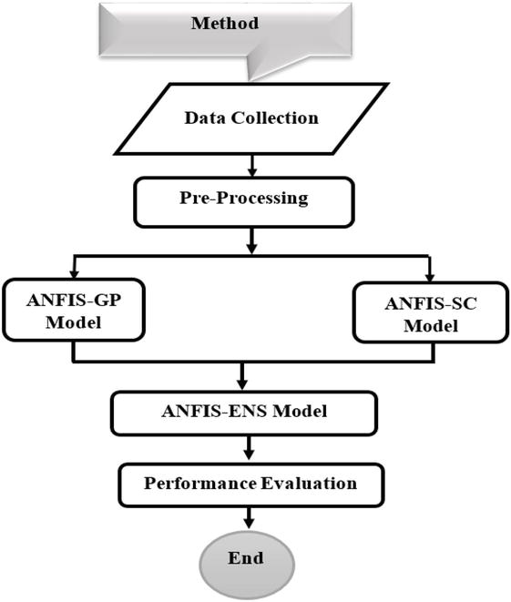
The step-by-step procedure of the entire study is illustrated in the flow chart, as shown in Figure 1. Our approach introduces three distinct ANFIS models. The first model is trained using the grid-partitioning optimization method (ANFIS-GP), while the second model adopts the sub clustering optimization technique (ANFIS-SC). To maximize the benefits of these optimization approaches, we create a third model by combining them in an ensemble manner (ANFIS-ENS). This ensemble configuration allows us to leverage the unique strengths of each model.

Figure 1.

Proposed methodology.

The subsequent sections elaborate on how we collected and preprocessed the data, along with the evaluation procedure used to measure the performance of our developed models. By following this comprehensive methodology, we aim to achieve accurate and reliable estimations of solar radiation.

The methodology is succinctly outlined in Figure 1 above and can be elaborated upon in greater detail below:

2.1 Data collection and preprocessing

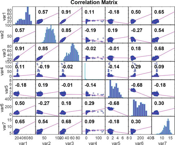
In this research, we collected a dataset containing daily solar radiation parameters for the entire year of 2018, spanning from January to December. The parameters consist of maximum temperature (Tmax), minimum temperature (Tmin), average temperature (T), and solar radiations (${\mathit{SR}}_{\mathit{k}}\mathit{,}{\mathit{SR}}_{\mathit{k}\mathit{-}1}\mathit{,}{\mathit{SR}}_{\mathit{k}\mathit{-}2}$). The study location, Kano, is positioned at a latitude of 12°03′N and a longitude of 12°32′E, with an altitude of approximately 472 meters above sea level. The average height of the study area is around 472.45 meters. To acquire the data, we obtained information from the Nigerian Meteorological Agency (NIMET). The original dataset encompassed various parameters, including average temperature (T), maximum temperature (Tmax), minimum temperature (Tmin), precipitation (R), wind speed (WS), relative humidity (RH), and solar radiation (SR). To ensure an optimal model, we evaluated the correlations between these parameters and selected those with a correlation greater than or equal to 50%. This approach helps avoid including irrelevant parameters that may not significantly impact the output. Figure 2 illustrates the correlation matrix, revealing a high correlation between var7 (representing solar radiation) and the first three variables, var1, var2, and var3 (representing mean, maximum, and minimum temperatures, respectively). Consequently, we only utilized these three variables for our modeling purposes.

Figure 2.

Correlation matrix.

In the context of our study, we have formulated a comprehensive model that incorporates a range of predictors, including mean, maximum, and minimum temperatures, along with solar radiation data from the preceding 2 days. This mathematical representation elegantly captures the interplay of these factors, empowering us to make accurate predictions and draw insightful conclusions. This is expressed mathematically as in Eq. (1) below:

$$M1={\mathit{SR}}_k\left(T,\mathit{\text{Tmax}},\mathit{\text{Tmin}},{\mathit{SR}}_{k-1},{\mathit{SR}}_{k-2}\right)$$E1

where M1 represents the developed model and ${\mathit{SR}}_{\mathit{k}}$ denotes the solar radiation to be predicted or the output of the model. The inputs of the model include:

• T, which represents the average temperature.

• Tmax, which signifies the maximum temperature.

• Tmin, which denotes the minimum temperature.

• ${\mathit{SR}}_{\mathit{k}\mathit{-}1}\mathit{\text{and}}{\mathit{SR}}_{\mathit{k}\mathit{-}2}$ representing the solar radiations for the preceding 2 days.

2.2 ANFIS-GP and ANFIS-SC

This section of the methodology involves the development of individual models, ANFIS-SC and ANFIS-GP, takes place. During this stage, the processed data is utilized for model development, with 70% of the data allocated for training, while the remaining 30% is designated for testing in each of the two models.

2.3 ANFIS-ENS model

This section of the methodology pertains to the ANFIS-ENS model. In this section, the strength of the individual models is combined. By doing so, ANFIS-ENS can harness its complementary capabilities to enhance overall accuracy.

2.4 Performance evaluation

The final section of the methodology involves performance evaluation. In this section, the accuracy of the model is scrutinized using a range of diverse performance metrics, this can be explained in Section 2.7 of the chapter.

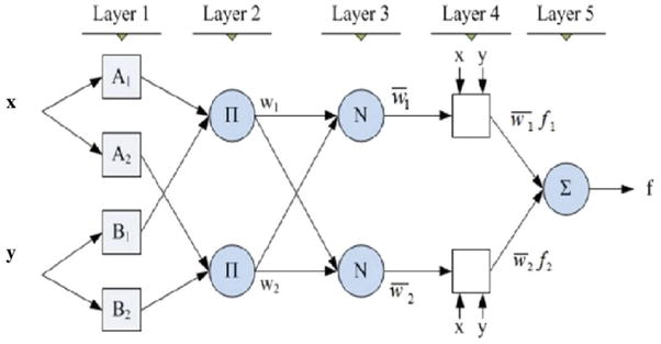
2.5 Adaptive neuro-fuzzy inference system (ANFIS)

The Adaptive Neuro-Fuzzy Inference System (ANFIS) is a powerful amalgamation of fuzzy logic and the learning capabilities of neural networks [35]. ANFIS encompasses three primary types: Mamdani, Sugeno, and Tsumoto, with Sugeno’s system being the most widely utilized [27, 36, 37]. In Fuzzy logic, input data are transformed into fuzzy values through the application of membership functions, where fuzzy values range from 0 to 1. The ANFIS model’s structure is formed by nodes functioning as membership functions (MFs) and rules that define the relationship between input and output. Various types of membership functions are available, including triangular, trapezoidal, Gaussian, and sigmoid. Among these, the Gaussian function (as shown in Eq. (4) below) is commonly employed [38].

$${\mathrm{V}}_{\mathrm{Li}}=\frac{1}{1+{\left[\raisebox{1ex}{$(X^{-\mathit{\alpha i})}$}\!\left/ \!\raisebox{-1ex}{$\mathit{\beta i}$}\right.\right]}^{2\mathit{\mu i}}}$$E2

The input variable x corresponds to the i node, where VLi represents the membership function, and βi and μi serve as the conditional parameters of this function. In the ANFIS framework, rules are formulated based on their antecedents (the “if” part) and consequents (the “then” part), and these rules are stored in a fuzzy-based rule system referred to as “the IF-THEN” rules. The rules for a Sugeno ANFIS model with two inputs (a and b) and one output f are illustrated by Eq. (5) and (6) [39].

$$\mathit{\text{Rule}}1;\mathit{\text{If}}x\mathit{\text{is}}{P}_1\mathit{\text{and}}y\mathit{\text{is}}{Q}_1,\mathit{\text{then}}{f}_1=P_{1}x+q_{1}y+r_1$$E3

$$\mathit{\text{Rule}}2;\mathit{\text{If}}x\mathit{\text{is}}{P}_2\mathit{\text{and}}y\mathit{\text{is}}{Q}_2\mathit{\text{then}}{f}_2=P_{2}x+q_{2}x+r_2$$E4

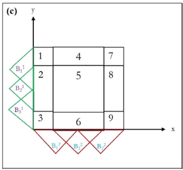
${\mathit{P}}_1$, ${\mathit{P}}_2$, $\mathit{\text{is}}{\mathit{Q}}_1$, and $\mathit{\text{is}}{\mathit{Q}}_2$ are referred to as fuzzy sets, while ${\mathit{f}}_1$ and ${\mathit{f}}_2$ represent the output within the fuzzy region. The design parameters, ${\mathit{r}}_1$ and ${\mathit{r}}_2$, are derived during the training process. The architecture of an ANFIS with two inputs (x and y) and one output (f) is depicted in Figure 3a. An elaborate investigation into ANFIS is presented by Mature et al. [27]. The goal is to minimize the objective function, as illustrated in Figure 4, before computing new fuzzy clusters. The fuzzifier exponent, P, lies between 0 and 1, while c represents the number of clusters. N denotes the number of data points, and a signifies the cluster centers.

Figure 3.

ANFIS structure with two inputs, one output, and two rules [40].

Figure 4.

Grid partitioning having 2 inputs with k = 3 [42].

In general, ANFIS comprises five distinct layers, illustrated in Figure 1, which are denoted as follows: the input layer, the layer for membership functions, the fuzzification layer, the defuzzification layer, and the normalization layer. This system operates with two inputs, specifically referred to as “x” and “y.” In this context, A1 and B1 represent fuzzy sets, while p1, q1, and r1 are design parameters, where i takes on values of 1 and 2.

The first layer within the ANFIS structure is the membership layer. In this layer, all nodes are adaptive, and it is responsible for generating membership grades for each input. This functionality is represented in equation above.

Moving on to the subsequent layer, it involves straightforward multiplication and is composed of fixed nodes. The mathematical representation of this layer can be expressed as follows:

$${\mathit{O}}_{2,\mathit{i}}={\mathit{w}}_{\mathit{i}}={\mathit{\mu }}_{\mathit{Ai}}\left(\mathit{x}\right)\times {\mathit{\mu }}_{\mathit{Bi}}\left(\mathit{x}\right)\mathit{i}=1,2$$E5

In the subsequent layer, there is a fixed node dedicated to normalization. This layer is responsible for standardizing the output generated by the second layer. The operation can be illustrated using the following equation:

$${\mathit{O}}_{3,\mathit{i}}=\overline{\mathit{w}}=\frac{{\mathit{w}}_{\mathit{i}}}{{\mathit{w}}_1+{\mathit{w}}_2}\mathit{i}=1,2$$E6

In this context, the firing level of node “i” is represented by ${\mathit{w}}_{\mathit{i}\mathit{.}}$

The fourth layer has the ability to streamline the result of the normalized output from the third layer. This layer adjusts itself dynamically, and you can express its output using the following equation:

$$O_{4,i}=\overline{w}{f}_i=\overline{w_i}\left(p_1+q_1+r_1\right)i=1,2$$E7

The last layer consists of a single fixed node, responsible for summing all incoming inputs. Ultimately, you can represent the overall result using the following equation:

$$O_{5,i}=\sum _{i=1}^2\overline{w}{f}_i=\frac{w_1{f}_1+w_2{f}_2}{w_1+w_2}$$E8

ANFIS exhibits improved learning capabilities due to the incorporation of back propagation and least square methods, which improve the system’s accuracy and expedite convergence. As previously mentioned, there are six consequent parameters in this system when assuming the utilization of bell-shaped membership functions. The primary goal within this ANFIS system is to optimize these parameters to achieve the lowest cost. Specifically, back propagation is employed to modify the parameters in the first layer, while the least square approach is responsible for fine-tuning the parameters in the fourth layer [41].

2.5.1 Grid partitioning (GP)

In ANFIS-GP, the integration of ANFIS and grid-partitioning techniques is employed. The grid-partitioning method involves dividing the data into smaller subsets, referred to as grid data, based on the type of membership function (MFS) in each dimension. The chart representation of ANFIS-GP, with three partitions (k = 3), is depicted in Figure 3b. Initially, ANFIS-GP starts with zero output and gradually learns distinct fuzzy set rules and functions through the training process [27]. To determine the initial fuzzy sets and parameters, the least square method is utilized, considering the partitions and MF types [43].

2.5.2 Subtractive clustering (SC)

The integration of ANFIS and SC yields ANFIS-SC. Each individual data point is considered a possible cluster center. As a result, a point surrounded by multiple neighboring points exhibits a higher potential value. To identify the first cluster center, a density measure (${\mathit{d}}_{\mathit{i}}$) is defined in Eq. (9) below, and the data set point with the highest density or potential value is selected as the initial cluster center [44].

$${\mathit{d}}_{\mathit{i}}=\sum _{\mathit{K}=1}^{\mathit{N}}\mathit{exp}\left(-{\left(\frac{2}{{\mathit{r}}_0}\right)}^2.{‖{\mathit{x}}_{\mathit{i}}-{\mathit{x}}_{\mathit{k}}‖}^2\right)$$E9

The data point ${\mathit{x}}_{\mathit{i}}$ is regarded as the cluster center, while ${\mathit{x}}_{\mathit{k}}$ represents the remaining data points within the influence radius, which is used to determine the initial cluster center. To calculate the new density measurement, Eq. (10) below is utilized [45].

$${\mathit{d}}_{\mathit{\text{inew}}}={\mathit{d}}_{\mathit{i}}-{\mathit{d}}_1^{\prime }.\mathit{exp}\left(-\frac{\left(-{‖{\mathit{x}}_{\mathit{i}}-{\mathit{x}}_1^{\prime }‖}^2\right)}{{\left(\frac{{\mathit{r}}_{\mathit{b}}}{2}\right)}^2}\right)$$E10

The constant value ${\mathit{r}}_{\mathit{b}}$ defines the neighborhood range within which the potential will steadily decrease. Subsequent data points after the first cluster center experience a significant decrease in potential and become less likely to be chosen as subsequent cluster centers. Selecting the appropriate influential radius is crucial as it determines the number of clusters. The optimal value for ${\mathit{r}}_{\mathit{a}}$ should fall within the range of 0.1 to 2 [46], and specifically, ${\mathit{r}}_{\mathit{a}}$ equals 1.25 times ${\mathit{r}}_{\mathit{b}}$ [47]. Larger clusters will result in the development of more rules, making it important to avoid very small radii. Therefore, careful consideration in choosing the influential radius is vital for effective clustering.

2.6 Ensemble machine learning

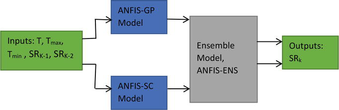
Ensemble machine learning emerges as a valuable approach to address the varying levels of accuracy exhibited by individual models, owing to their distinct robustness and constraints. This diversity of performance may lead to unsatisfactory outcomes in certain cases. Consequently, the adoption of ensemble techniques has become widespread across diverse fields, encompassing science, engineering, social and management sciences, health sciences, and beyond [17]. Ensemble methods involve the combination of both heterogeneous and homogeneous models, effectively harnessing their collective predictive power. Instead of relying solely on standalone models, ensemble techniques integrate the individual outputs of these models as new input variables, aiming to enhance the final performance skills of the simple models. Numerous empirical studies have consistently demonstrated that ensemble approaches yield superior results, particularly when confronted with complex and intricate problems. By leveraging the advantages of ensemble machine learning, practitioners can significantly elevate the reliability and efficacy of their solutions, providing robust and accurate solutions to multifaceted challenges. Embracing the potential of ensemble methods opens up new possibilities for advancing predictive modeling and decision-making processes across various domains. In this research, the ensemble model, ANFIS-ENS, combines the strengths of the individual models known as ANFIS-GP and ANFIS-SC. By combining these two paradigms, the ensemble can take advantage of their complementary capabilities and thus enhance the overall performance of the model.

Above is a block diagram of the developed model. The processed inputs of the model, T, Tmax, Tmin, SR_K-1, and SR_K-2, are trained using the individual models. Within each of these individual models, solar radiation is predicted, and the output is obtained. The outputs of the individual models, ANFIS-GP and ANFIS-SC, are now used as inputs for the Meta model known as ANFIS-ENS.

2.7 Performance evaluation

The evaluation of model performance throughout both training and testing stages involves the utilization of four widely recognized statistical metrics: the correlation coefficient (R), determination coefficient (DC), mean-squared-error (MSE), root-mean-squared-error (RMSE), and mean absolute error (MAE). These essential metrics provide valuable insights into the models’ predictive accuracy, enabling a comprehensive assessment of their efficacy and generalization capabilities. The computation of these metrics is facilitated by employing Eq. (11)–(13) [48, 49, 50].

2.7.1 Pearson correlation coefficient (R)

The Pearson correlation coefficient is a measure that evaluates the magnitude or strength and direction of the linear relationship between two variables. It signifies the extent to which one variable changes when the other variable changes, and is expressed as numerical value between −1 and 1 [18].

A Pearson correlation coefficient of −1 signifies a perfect negative linear relationship, which means that when one variable decreases, the other variable increases in a linear fashion. A Pearson correlation coefficient of +1 signifies a superb positive linear relationship between the two variables, which means that when one variable increases, the other variable also increases in a linear fashion. A Pearson correlation coefficient of 0 indicates no linear relationship between the two variables. The Pearson correlation coefficient can be computed by the following equation:

$$\mathit{R}=\frac{\sum \left(\left({\mathit{x}}_{\mathit{i}}-\overline{\mathit{x}}\right)-\left({\mathit{y}}_{\mathit{i}}-\overline{\mathit{y}}\right)\right)}{\sqrt{\sum {\left({\mathit{x}}_{\mathit{i}}-\overline{\mathit{x}}\right)}^2\sum {\left({\mathit{y}}_{\mathit{i}}-\overline{\mathit{y}}\right)}^2}}$$E11

Where ${\mathit{x}}_{\mathit{i}}$ is independent variable, ${\mathit{y}}_{\mathit{i}}$ is dependent variable, $\overline{\mathit{x}}$ is the mean of variable ${\mathit{x}}_{\mathit{i}}$ values, and $\overline{\mathit{y}}$ is the mean of variable ${\mathit{y}}_{\mathit{i}}$ values.

2.7.2 Coefficient of determination (DC)

Coefficient of determination, also known as R-squared, is a statistical metric that evaluates how effectively a regression model fits the data points [13]. It is a value ranging from 0 to 1 that symbolizes the proportion of the variance in the dependent variable that can be predicted from the independent variable(s). A DC value of 1 represents a perfect fit of the regression predictions, while a DC value of 0 suggests that the model does not account for any of the dependent variable’s variation. A higher DC value indicates a better fit of the model to the data, moreover, DC is calculated as the ratio of the explained variance to the total variance. The explained variance is the variation in the dependent variable that is explained by the independent variable(s), while the total variance is the variation in the dependent variable that is not explained by the independent variable(s). Below is the mathematical expression for DC:

$$\mathit{DC}=1-\frac{\sum {\left({\mathit{x}}_{\mathit{i}}-{\widehat{\mathit{x}}}_{\mathit{i}}\right)}^2}{\sum {\left({\mathit{x}}_{\mathit{i}}-{\overline{\mathit{x}}}_{\mathit{i}}\right)}^2}$$E12

2.7.3 Mean squared error

The mean squared error (MSE), also known as mean squared deviation (MSD), for an estimator (a method used to estimate an unobserved quantity) evaluates the average of the squared discrepancies, which is essentially the average of the squared differences between the estimated values and the true value. MSE serves as a risk function, representing the anticipated value of the squared error loss.

$$\mathit{MSE}=\frac{\sum {\left({\mathit{x}}_{\mathit{i}}-{\widehat{\mathit{x}}}_{\mathit{i}}\right)}^2}{\mathit{n}}$$E13

2.7.4 Root mean square error

The root mean square error (RMSE) is a widely employed metric for assessing the precision of a statistical model or prediction algorithm. It quantifies the disparity between anticipated and observed values within a dataset [51]. To compute RMSE, one takes the square root of the average of the squared disparities between predicted and actual values. This metric is denominated in the same units as the data, providing an indication of the average magnitude of deviations between predicted and actual values. The formula for RMSE is as follows:

$$\mathit{\text{RMSE}}=\sqrt{\frac{\sum {\left({\mathit{x}}_{\mathit{i}}-{\widehat{\mathit{x}}}_{\mathit{i}}\right)}^2}{\mathit{n}}}$$E14

2.7.5 Mean absolute error

The mean absolute error (MAE) is a measurement used to determine the average discrepancy between predicted values and actual values within a dataset, without considering the direction of the errors. This is computed by finding the mean of the absolute differences between the predicted and actual values [52]. In mathematical terms, MAE can be expressed as:

$$\mathit{MAE}=\frac{1}{\mathit{n}}\sum \left|{\mathit{x}}_{\mathit{i}}-{\widehat{\mathit{x}}}_{\mathit{i}}\right|$$E15

For $\mathit{i}=1,2,3\dots .\mathit{n}$ Where ${\mathit{x}}_{\mathit{i}}$,${\widehat{\mathit{x}}}_{\mathit{i}}$, ${\overline{\mathit{x}}}_{\mathit{i}}$, and n represent the original values, predicted values, the average value of the original data, and the total number of data instances, respectively.

3. Results and discussion

Table 1 demonstrates a high coefficient of determination (DC) ranging from 80 to 95%, which is highly commendable for a predictive model. The independent variables include RH, WS, Tmin, Tmax, and T. Analyzing the correlation matrix between SR and each input reveals a strong and positive correlation between SR and Tmin, Tmax, and T. Consequently, a model of SR incorporating these temperature variables, known as M1, has been developed. The statistical indicators (DC, RMSE, DC, MSE, and MAE) in Table 1 outline the model’s accuracy. The performance of individual models, namely ANFIS-GP, ANFIS-SC, and their combination (ensemble), has been thoroughly evaluated. During the evaluation process, 80% of the data is used for training, while the remaining 20% is reserved for testing. Various statistical metrics are employed to assess the models’ performance, focusing on both the goodness of fit and performance error. The results are presented in Table 1, which clearly indicates that model M1 provides a significantly accurate prediction of solar radiation. Additionally, the ensemble method outperforms the individual models, with a DC of 95% compared to 80% for ANFIS-SC and 93% for ANFIS-GP.

Training
	Methods	R	DC	MSE	RMSE	MAE
M1	GP	0.964419	0.930103	0.030505	0.174656	0.119767
	SC	0.898913	0.808045	0.083774	0.289437	0.203251
	ENS	0.97688	0.954294	0.019947	0.141235	0.101438
Testing
M1	GP	0.959621	0.920873	0.027558	0.166006	0.11559
	SC	0.863194	0.745104	0.088774	0.297949	0.211935
	ENS	0.971104	0.943043	0.019837	0.140843	0.103832

Table 1.

Performance evaluation of the models.

The result highlights the efficacy of ensemble approaches in enhancing predictive accuracy and reaffirms their value in practical applications.

The provided results showcase the performance of the model using different optimization algorithms for training and testing. The three methods, ANFIS-GP, ANFIS-SC, and the ensemble (ENS), were evaluated based on key statistical metrics, such as correlation coefficient (R), determination coefficient (DC), mean squared error (MSE), root mean squared error (RMSE), and mean absolute error (MAE). It is evident from the training and testing results that the ensemble method (M1-ENS) consistently outperforms the individual ANFIS-SC (M1-SC) and ANFIS-GP (M1-GP) models in terms of R, DC, MSE, RMSE, and MAE. The ensemble approach showcases higher values for R and DC, indicating a stronger correlation and better determination capabilities. Additionally, it demonstrates lower values for MSE, RMSE, and MAE, which signify reduced prediction errors and enhanced accuracy.

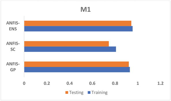
To provide a clearer understanding of the predictive model’s performance error, specifically in terms of RMSE, a bar chart can visually illustrate the comparative analysis. Figure 5 displays the RMSE values for all training algorithms applied to model M1, demonstrating that they fall within the acceptable range during both the training and testing stages. This reaffirms the models’ exceptional ability to effectively capture the complex relationship between the predictors and solar radiation (Figure 6).

Figure 5.

Block diagram of the models.

Figure 6.

Performance comparison of model M1.

From the graph above, it can be seen that ANFIS-ENS, having the least RMSE, outperformed both the individual models, ANFIS-GP and ANFIS-SC. The performance ranking of the models in M1 for both training and testing is as follows: ENS > GP > SC.

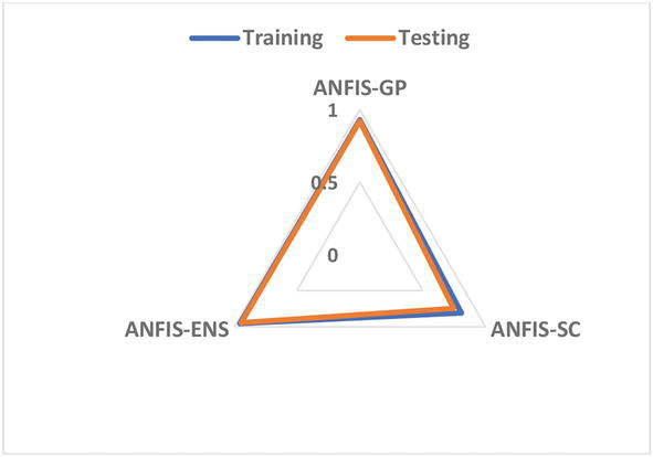
The radar chart in Figure 7 provides a clear view of the comparison of the models ANFIS-GP, ANFIS-SC, and ANFIS-ENS based on the coefficient of determination (DC). The models with their DC values closer to 1 generally have more accuracy. Hence, the order of accuracy of the three models developed can be ranked in terms of accuracy from highest to lowest as $\mathit{ENS}\mathit{>}\mathit{GP}\mathit{>}\mathit{SC}$.

Figure 7.

Radar plot to compare the performance of the models.

In the present study, we developed an ANFIS Ensemble model to predict solar radiation in Kano State, Nigeria. The achieved accuracy of 0.9543 (DC values) demonstrates the effectiveness of our model. To discuss the results, let us compare them with the accuracies reported in the previous studies listed in the Table 2 below.

Authors	Model type	Input parameters	Location	DC values
Yohanna et al. [53]	Empirical	3	Nigeria	0.608
Abdalla [54]	Empirical	4	Bahrain	0.780
Ramedani [55]	ANFIS	3	Iran	0.808
Olatomiwa et al. [56]	ANFIS	3	Nigeria	0.8544
Sajid and Ali [38]	ANFIS	3	Abu Dhabi	0.860
Sani S et al. [57]	ANFIS	4	Nigeria	0.8688
Present Study	ANFIS ENSEMBLE	3	Nigeria	0.9543

Table 2.

Comparison between the present study and the previous studies available from the literature.

Yohanna et al. [53] presented an empirical model for solar radiation prediction in Nigeria, achieving an accuracy of 0.608. This relatively low accuracy may be attributed to the limitations of empirical models in capturing complex nonlinear relationships present in solar radiation data. Our ANFIS Ensemble model, with its ability to handle nonlinear relationships, significantly outperformed this empirical model.

Abdalla [54] also employed an empirical model, but in the context of Bahrain, achieving an accuracy of 0.780. Again, our ANFIS Ensemble model surpassed this accuracy, highlighting the advantages of using ANFIS techniques for solar radiation prediction.

Ramedani [55] utilized an ANFIS model in Iran and achieved an accuracy of 0.808. While our model demonstrates higher accuracy, it is essential to consider the differences in geographical locations and solar radiation patterns between Iran and Nigeria, which can influence prediction performance.

Olatomiwa et al. [56] developed an ANFIS model for solar radiation prediction in Nigeria, attaining an accuracy of 0.8544. Although their model performed well, our ANFIS Ensemble model surpassed it by a significant margin, illustrating the benefits of combining multiple ANFIS models.

Sajid and Ali [38] utilized an ANFIS model in Abu Dhabi, achieving an accuracy of 0.860. Again, our ANFIS Ensemble model outperformed their model, highlighting the effectiveness of our approach.

Sani S et al. [58] employed an ANFIS model with four input parameters for solar radiation prediction in Nigeria, attaining an accuracy of 0.8688. Our ANFIS Ensemble model exhibited a higher accuracy, showcasing the advantages of our ensemble approach even with a reduced number of input parameters.

In summary, our ANFIS Ensemble model achieved an accuracy of 0.9543, outperforming all the models compared in the Table 2. This indicates the superiority of our approach in accurately predicting solar radiation in Kano State, Nigeria. The ensemble technique, combining the strengths of individual ANFIS models, allowed us to achieve a more robust and accurate prediction. These results underscore the relevance and significance of our research, providing valuable insights into renewable energy systems, agricultural planning, and climate modeling in Kano State.

4. Conclusion

This study explored the application of ensemble machine-learning algorithms for predicting solar radiation in Kano, Nigeria. The primary objective was to develop robust machine-learning models for estimating solar radiation. Meteorological data consisting of four parameters, namely Maximum-Temperature (Tmax), Minimum-Temperature (Tmin), Mean-Temperature (Tmean), and solar radiation, were utilized. The data covered daily average values over a period of 12 months (January to December 2018). To enhance the predictive performance, the study employed an ensemble model by combining two optimization techniques: sub-clustering and grid-partitioning methods. The results were assessed using various evaluation metrics such as “R, DC, MSE, RMSE, and MAE” to ensure a comprehensive analysis and avoid bias, leading to better generalization of accuracy. The findings demonstrate that utilizing the ensemble approach yields more credible and acceptable outcomes. This research contributes to the development of reliable predictive models for solar radiation estimation, which can have significant implications in various applications and decision-making processes related to renewable energy utilization. Overall, the combination of ensemble machine learning and meteorological data proves to be a promising approach for accurate solar radiation prediction in the specific region of Kano, Nigeria.

Acknowledgments

The authors would like to appreciate the effort of the Nigerian Meteorological Agency (NIMET) for providing the required data for this research.

Recommendations

The following will be recommended for future work:

1. Application of the ensemble approach on hourly solar radiation estimation instead of the daily averages.

2. Other sophisticated machine learning methods such as hybrid machine learning, emotional neural network, and deep learning technique will be implemented with a larger dataset to have a more general view.

3. Employ the Internet of Things technologies (IoT) along with smart sensors and sensor networks to achieve a real-time data collection and solar radiation estimation.

4. The research will also consider more cities in Nigeria.

References

1.Kosmadakis G, Karellas S, Kakaras E. Renewable and Conventional Electricity Generation Systems: Technologies and Diversity of Energy Systems. London: Springer; 2013. DOI: 10.1007/978-1-4471-5595-9
2.Prakash R, Krishnan I. Energy, economics and environmental impacts of renewable energy systems energy, economics and environmental impacts of renewable energy systems. Renewable and Sustainable Energy Reviews. 2009;13:2716-2721. DOI: 10.1016/j.rser.2009.05.007
3.Panwar NL, Kaushik SC, Kothari S. Role of renewable energy sources in environmental protection: A review. Renewable and Sustainable Energy Reviews. 2011;15(3):1513-1524. DOI: 10.1016/j.rser.2010.11.037
4.Dowell J, Pinson P. Very-Short-Term Probabilistic Wind Power Forecasts by Sparse Vector Autoregression. IEEE Transactions on Smart Grid. 2016;7:763-770. DOI: 10.1109/TSG.2015.2424078
5.I. Renewable and E. Agency. Renewable Energy Statistics 2018 Statistiques D’ Énergie Renouvelable 2018 Estadísticas De Energía. I. Renewable and E. Agency; 2018
6.Reddy SS. Optimization of renewable energy resources in hybrid energy systems. 2017;7:43-60. DOI: 10.13052/jge1904-4720.7123
7.Alkesaiberi AH, Fouzi Sun Y. Efficient Wind Power Prediction Using Machine Learning Methods: A Comparative Study. 2022;15. DOI: 10.3390/en15072327
8.Jahani B. A Comparison between the Application of Empirical and ANN Methods for Estimation of Daily Global Solar Radiation in Iran; 2018;13. DOI: 10.1007/s12517-020-05437-0
9.Yaniktepe B, Kara O, Ozalp C. Technoeconomic evaluation for an installed small-scale photovoltaic power plant. 2017;2017
10.R. Energy. Renewable Energy Policies in a Time of Transition. ISBN: 9789292600617
11.Ahmed R, Sreeram V, Mishra Y, Arif MD. A review and evaluation of the state-of-the-art in PV solar power forecasting: Techniques and optimization. Renewable and Sustainable Energy Reviews. 2020;124:109792. DOI: 10.1016/j.rser.2020.109792
12.Dey BK, Khan I, Abhinav MN, Bhattacharjee A. Mathematical modelling and characteristic analysis of solar PV cell. In: 7th IEEE Annu. Inf. Technol. Electron. Mob. Commun. Conf. IEEE IEMCON 2016. 2016. DOI: 10.1109/IEMCON.2016.7746318
13.Teke A, Ba H, Çelik Ö. Evaluation and performance comparison of different models for the estimation of solar radiation. 2015;50:1097-1107. DOI: 10.1016/j.rser.2015.05.049
14.Almorox J, Hontoria C, Benito M. Models for obtaining daily global solar radiation with measured air temperature data in Madrid (Spain). Applied Energy. 2011;88(5):1703-1709. DOI: 10.1016/j.apenergy.2010.11.003
15.Ali-Ou-Salah H, Oukarfi B, Bahani K, Moujabbir M. A new hybrid model for hourly solar radiation forecasting using daily classification technique and machine learning algorithms. Mathematical Problems in Engineering. 2021;2021. DOI: 10.1155/2021/6692626
16.Akhter MN, Mekhilef S, Mokhlis H, Shah NM. Review on forecasting of photovoltaic power generation based on machine learning and metaheuristic techniques. IET Renewable Power Generation. 2019;13(7):1009-1023. DOI: 10.1049/iet-rpg.2018.5649
17.Zhou Y, Liu Y, Wang D, Liu X, Wang Y. A review on global solar radiation prediction with machine learning models in a comprehensive perspective. Energy Conversion and Management. 2021;235(13):113960. DOI: 10.1016/j.enconman.2021.113960
18.Fraihat H, Almbaideen AA, Al-Odienat A, Al-Naami B, De Fazio R, Visconti P. Solar radiation forecasting by Pearson correlation using LSTM neural network and ANFIS method: Application in the west-Central Jordan. Future Internet. 2022;14(3). DOI: 10.3390/fi14030079
19.Chen W, Li DH, Li S, Lam JC. Estimating hourly global solar irradiance using artificial neural networks - a case study of Hong Kong. IOP Conference Series: Materials Science and Engineering. 2019;556(1):012043. DOI: 10.1088/1757-899X/556/1/012043
20.Guermoui M, Rabehi A, Lalmi D. Multi-step ahead forecasting of daily solar radiation components in Saharan climate multi-step ahead forecasting of daily solar radiation components in Saharan climate. International Journal of Ambient Energy. 2018;41:1-23. DOI: 10.1080/01430750.2018.1490349
21.Linares-rodríguez A, Ruiz-arias JA, Pozo-vázquez D, Tovar-pescador J. Generation of synthetic daily global solar radiation data based on ERA-interim reanalysis and arti fi cial neural networks. Energy. 2011;36(8):5356-5365. DOI: 10.1016/j.energy.2011.06.044
22.Sözen A, Arcaklioglu E, Özalp M. Estimation of solar potential in Turkey by artificial neural networks using meteorological and geographical data. Energy Conversion and Management. 2004;45(18–19):3033-3052. DOI: 10.1016/j.enconman.2003.12.020
23.Piri J, Kisi O. Modelling solar radiation reached to the earth using ANFIS, NN-ARX, and empirical models (case studies: Zahedan and Bojnurd stations). Journal of Atmospheric and Solar-Terrestrial Physics. 2015;123:39-47. DOI: 10.1016/j.jastp.2014.12.006
24.Salcedo-Sanz S, Deo RC, Cornejo-Bueno L, Camacho-Gómez C, Ghimire S. An efficient neuro-evolutionary hybrid modelling mechanism for the estimation of daily global solar radiation in the sunshine state of Australia. Applied Energy. 2018;209:79-94. DOI: 10.1016/j.apenergy.2017.10.076
25.Mohammadi K, Shamshirband S, Hossein M, Amjad K, Petkovic D. Support vector regression based prediction of global solar radiation on a horizontal surface. 2015;91:433-441. DOI: 10.1016/j.enconman.2014.12.015
26.Naderloo L. Prediction of solar radiation on the horizon using neural network methods, ANFIS and RSM (case study: Sarpol-e-Zahab township, Iran). Journal of Earth System Science. 2020;129(1). DOI: 10.1007/s12040-020-01414-z
27.Wang L et al. Prediction of solar radiation in China using different adaptive neuro-fuzzy methods and M5 model tree. International Journal of Climatology. 2017;37(3):1141-1155. DOI: 10.1002/joc.4762
28.Cobos FF et al. Assessment of the impact of meteorological conditions on pyrheliometer calibration. Solar Energy. 2018;168:44-59. DOI: 10.1016/j.solener.2018.03.046
29.Yildirim A, Bilgili M, Ozbek A. One-hour-ahead solar radiation forecasting by MLP, LSTM, and ANFIS approaches. Meteorology and Atmospheric Physics. 2023;135(1):1-17. DOI: 10.1007/s00703-022-00946-x
30.Tao H et al. Global solar radiation prediction over North Dakota using air temperature: Development of novel hybrid intelligence model. Energy Reports. 2021;7:136-157. DOI: 10.1016/j.egyr.2020.11.033
31.Abba SI, Pham QB, Saini G, Thi N, Linh T, and Ahmed AN. Implementation of Data Intelligence Models Coupled with Ensemble Machine Learning for Prediction of Water Quality Index; 2020
32.Selin AGU, Abba ISI. A novel multi - model data - driven ensemble technique for the prediction of retention factor in HPLC method development. Chromatographia. 2020;83:933-945. DOI: 10.1007/s10337-020-03912-0
33.Ammar MI et al. Improving the prediction of solar radiation using ANFIS optimization ensemble; 1(5):1-13. DOI: 10.1007/978-3-320-59427-9
34.Sciences H, Journal J, August H. Comparative implementation between neuro-emotional genetic algorithm and novel ensemble computing techniques for modelling dissolved oxygen comparative implementation between neuro- emotional genetic algorithm and novel ensemble computing techniques for m. Hydrological Sciences Journal. 2021;66(10):1-13. DOI: 10.1080/02626667.2021.1937179
36.Salisu S, Mustafa MW, Mustapha M. Predicting Global Solar Radiation in Nigeria Using Adaptive Neuro-Fuzzy Approach. Vol. 2. Cham: Springer; 2018. DOI: 10.1007/978-3-319-59427-9
37.Abdulkadir RA, Wudil T, Gaya MS, Shauket S, Muhammad UG. Effluents quality prediction by using nonlinear dynamic block-oriented models : A system identification approach effluents quality prediction by using nonlinear dynamic block-oriented models: A system identification approach. 2021;218:52-62. DOI: 10.5004/dwt.2021.26983
38.Hussain S, Al Alili A. Soft computing approach for solar radiation prediction over Abu Dhabi, UAE: A comparative analysis. In: International Conference on Smart Energy Grid Engineering SEGE. Vol. 2015. 2015. pp. 1-6. DOI: 10.1109/SEGE.2015.7324613
39.Rathnayake N, Dang TL, Hoshino Y. A novel optimization algorithm: Cascaded adaptive neuro-fuzzy inference system. International Journal of Fuzzy Systems. 2021;23(7):1955-1971. DOI: 10.1007/s40815-021-01076-z
40.Maroufpoor S, Shauket S, Al-ansari N, Malik A. A novel hybridized neuro-fuzzy model with an optimal input combination for dissolved oxygen estimation. 2022;10:929707
41.Zubaidi SL et al. A novel methodology for prediction urban water demand by wavelet denoising and adaptive neuro-fuzzy inference system approach. Water (Switzerland). 2020;12(6). DOI: 10.3390/w12061628
42.Yavarian K, Mohammadian A, Hashemi F. Adaptive neuro fuzzy inference system PID controller for AVR system using SNR-PSO optimization adaptive neuro fuzzy inference system PID controller for AVR system using SNR-PSO optimization. International Journal on Electrical Engineering and Informatics. 2016;7:394-408. DOI: 10.15676/ijeei.2015.7.3.3
43.Yaseen ZM, Ramal MM. Hybrid Adaptive Neuro-Fuzzy Models for Water Quality Index Estimation; 2018
44.Choubin B, Darabi H, Rahmati O, Sajedi-hosseini F, Kløve B. Science of the Total Environment River suspended sediment modelling using the CART model: A comparative study of machine learning techniques. Science of the Total Environment. 2018;615:272-281. DOI: 10.1016/j.scitotenv.2017.09.293
45.Taylor P, Bezdek JC. Cluster validity with fuzzy sets. Journal of Cybernetics. 2008;3:37-41. DOI: 10.1080/01969727308546047
46.Halkidi M, Batistakis Y, Vazirgiannis M. Cluster validity methods: Part I. 2002;31(2):40-45
47.Arbelaitz O, Gurrutxaga I, Muguerza J. An extensive comparative study of cluster validity indices. 2013;46:243-256. DOI: 10.1016/j.patcog.2012.07.021
48.Zang H, Liu L, Sun L, Cheng L, Wei Z, Sun G. Short-term global horizontal irradiance forecasting based on a hybrid CNN-LSTM model with spatiotemporal correlations. Renewable Energy. 2020;160:26-41. DOI: 10.1016/j.renene.2020.05.150
49.Antor AF, Wollega ED. Comparison of machine learning algorithms for wind speed prediction. In: Proceedings of the 5th NA International Conference on Industrial Engineering and Operations Management Detroit, Michigan, USA, August 10 - 14, 2020. 2020. pp. 857-866
50.He C et al. Improving solar radiation estimation in China based on regional optimal combination of meteorological factors with machine learning methods. Energy Conversion and Management. 2020;220:113111. DOI: 10.1016/j.enconman.2020.113111
51.Lawan SM, Abidin WAWZ, Chai WY, Baharun A, Masri T. Different models of wind speed prediction: A comprehensive review. 2014;5(1)
52.Dalianis H. Evaluation metrics and evaluation. Clinical Text Mining. 2018;1967:45-53. DOI: 10.1007/978-3-319-78503-5_6
53.Yohanna JK, Itodo IN, Umogbai VI. A model for determining the global solar radiation for Makurdi, Nigeria. Renewable Energy. 2011;36(7):1989-1992. DOI: 10.1016/j.renene.2010.12.028
54.Taylor P, Abdalla YAG. New correlations of global solar radiation with meteorological parameters for Bahrain new correlations of global solar radiation with meteorological. International Journal of Solar Energy. 2007;2013:37-41
55.Ramedani Z, Omid M, Keyhani A, Shamshirband S, Khoshnevisan B. Potential of radial basis function based support vector regression for global solar radiation prediction. Renewable and Sustainable Energy Reviews. 2014;39:1005-1011. DOI: 10.1016/j.rser.2014.07.108
56.Olatomiwa L, Mekhilef S, Shamshirband S, Petković D. Adaptive neuro-fuzzy approach for solar radiation prediction in Nigeria. Renewable and Sustainable Energy Reviews. 2015;51:1784-1791. DOI: 10.1016/j.rser.2015.05.068
57.Salisu S, Mustafa MW, Mustapha M. Predicting global solar radiation in Nigeria using adaptive neuro-fuzzy approach. Lecture Notes on Data Engineering and Communications Technologies. 2018;5:513-521. DOI: 10.1007/978-3-319-59427-9_54
58.Gaya MS, Wahab NA, Sam Y, Samsuddin SI. Comparison of ANFIS and neural network direct inverse control applied to wastewater treatment system. 2014;845:543-548. DOI: 10.4028/www.scientific.net/AMR.845.543
Written By
Ammar Muhammad Ibrahim, Salisu Muhammad Lawan, Rabiu Abdulkadir, Nazifi Sani Shuaibu, Muhammad Uzair, Musbahu Garba Indabawa, Masud Ibrahim and Abdullahi Mahmoud Aliyu
Submitted: 08 August 2023Reviewed: 11 September 2023Published: 25 March 2024