Lanchester’s Fighting Strength as a Battle Outcome Predictor Applied to a Simple Fire and Manoeuvre Wargame

Abstract

Lanchester’s equations developed a mathematical understanding of the process of combat, leading to the concept of ‘fighting strength’, the product of fighting efficiency and numbers of troops squared. In this paper we demonstrate that ‘fighting strength’ is a key predictor of outcomes using a simple fire and manoeuvre wargame, set on a Mobius Strip. Lanchester’s equations are solved showing ‘saddle points’, where beneath defeat is certain and above which victory is certain. The influence of tactics is explored using experimental design. The probability of loss in the game with consecutive dice rolls is solved. ‘Fighting strength’ predicted the final result in 33 out of 34 wargames with asymmetric forces. In addition Lanchester’s equations also provide solutions for the % number of casualties in the wargames and the length of time each battle was fought. Based on initial pre-combat fighting efficiencies and numbers of troops between two opponents, a table of likely military strategies are presented to account for the differing ‘fighting strengths’ that best describe possible strategies that can succeed.

1. Introduction

I returned, and saw under the sun, that the race is not to the swift, nor the battle to the strong, neither yet bread to the wise, nor yet riches to men of understanding, nor yet favour to men of skill; but time and chance happeneth to them all. Ecclesiastes 9:11.

Ecclesiastes tells us that life, including the outcome of battles, has a stochastic element. The study of military history tells us, in addition, that the numbers of troops engaged, their quality, weapons and tactics, together with their morale significantly influences the outcome. In 1916, F.W. Lanchester [1] developed a mathematical understanding of the process of combat, and this is reviewed in Appendix A. The loss of active fighting troops with fire exchange follows a differential equation, whose solution leads to the concept of ‘fighting strength’ in a square law relationship.

$${}^{‘}\text{Fighting}{\text{strength}}^{’}=\mathrm{P}{\mathrm{N}}^2.$$E1

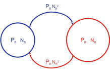
where P is the ‘efficiency’ or probability of hitting an opponent in a fire exchange, removing them from further combat, and N is the number of troops available to fight in the fire exchange. The simultaneous and continuous fire exchange in the battle leads to a steady reduction in numbers of combatants for each side with the outcome driven by the fighting strength. In the example below unless the Blue force has a significantly higher probability P_B of hitting an opponent in a fire exchange then the disparity in numbers compared to the Red force will eventually dominate (Figure 1).

Figure 1.

Schematic representation of the Lanchester model for combat for Red and Blue forces, with the area of the circle proportional to the number of troops N_B (Blue) & N_R (Red) in each force, and the probability of hitting an opponent P_B (Blue) and P_R (Red).

Lanchester’s equations suggest that the fighting strength of two opposing forces indicate the outcome of the battle before it takes place: the side with the greater fighting strength being able to eliminate its rival should it stand and fight to the end. Based on this, it is possible to devise a table of strategies [2] that looks at the best options for a Red force attacking a Blue force, by looking carefully at variations in combat efficiency and numbers and how these affect fighting strength.

The suggested battle strategies for a Red force fighting a Blue force based on Lanchester’s fighting strength include (Table 1).

	Lower efficiency (PR < PB) than Blue	Same efficiency (PR = PB) as Blue	Better efficiency (PR > PB) than Blue
Smaller numbers than Blue; NR < NB	Fabian strategy [5]; PR NR^2 ≪ PB NB^2	Fabian strategy [5], or tactics of division if unable to avoid battle [4]	Tactics of concentration[2]
Same numbers as Blue; NR = NB	Fabian strategy [5], or tactics of division if unable to avoid battle [4]	Tactics of division [4]	Tactics of concentration [2]
Higher numbers than Blue; NR > NB	Tactics of numbers [3]	Tactics of numbers [3]	Vernichtungsschlacht [1]; PR NR^2 ≫ PB NB^2

Table 1.

Classification of possible tactics for a Red force fighting a Blue force with underlying variations to fighting strength.

1. Vernichtungsschlacht—Battle of Annihilation. Move immediately to optimal firing range and destroy the Blue force, since P_R N_R² ≫ P_B N_B².

2. Tactics of concentration. Divide the Blue forces into smaller groups, so that the Red force has greater fighting strength in each battle against the smaller groups of Blue forces, destroying them in turn.

3. Tactics of numbers. Red forces can defeat a smaller Blue force by preventing them from dividing. Red forces (i.e. prevent Blue forces from using tactics of concentration against them), engaging at optimal firing range.

4. Tactics of division. Set up small battles more favourable to Red forces, in an attempt to reduce down the Blue force numbers. This could involve decoys, traps and surprise manoeuvres such as tunnels.

5. Fabian strategy—avoid pitched battles. Manoeuvre, engaging with Blue forces sparingly on best terms of engagement as possible in a war of attrition, since P_R N_R² ≪ P_B N_B².

Later we will explore the influence of such tactics on the outcome of a simple wargame.

Lanchester’s equations have been applied with success to many different historical battles including naval (Trafalgar [3, 4, 5], Dogger Bank [6], Jutland [7], Midway [8, 9, 10]); land (American Civil War [11, 12]), WW2 (Kursk [13, 14, 15, 16], Iwo Jima [17], Insurgency [18, 19, 20, 21, 22]); and air (WW2 Battle of Britain [23]). They have also been applied to social insect warfare [24, 25]. Additional papers that examine or extend the theory are listed in Appendix A. In this paper, we test the fighting-strength concept by introducing a simple manoeuvre-and-fire wargame, one that readily becomes a Vernichtungsschlacht—Battle of Annihilation—because of the playing surface.

2. Simple manoeuvre and fire wargame—Möbius Mayhem

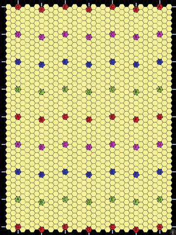
The map represents a space station that is a Möbius strip, a continuous featureless surface from which escape is not possible and which players representing Red and Blue forces of space marines seek to control. These forces are armed with direct fire weapons, with unlimited ammunition and whose probability of hitting an opponent increases as the range decreases (Figure 2).

Figure 2.

Playing surface for the Möbius Mayhem wargame.

The coloured and lettered hexes are ‘trapdoors’, which allow units to move up or down the surface to the corresponding coloured and lettered hex, which is normally 20 hexes vertically distant and with a mirrored translation in symmetry left to right, or vice versa. If a unit moves off the top of the map, it reappears at the bottom and vice versa since the surfaces join together. Likewise, if it moves off one of the sides, it reappears on the other side with a 20 hex vertically distant mirrored transition like the trapdoors. The switches in symmetry and the continuous nature of the playing surface is a function of being a Möbius strip [26] (without the mirror symmetry, the space would be the surface of a torus).

Players use a fixed turn sequence (IgoYougo). The sequence of play is Move, then Fire, based on the system described in [27]. Units that move cannot fire. They may move up to 5 hexes per turn (0 to 5 Movement Points, MP, allocation), and may pass through the same hex as another unit, but cannot remain in the same hex as another unit at the end of the turn. Going through a trapdoor and reappearing on the board elsewhere costs 1MP, and units cannot loiter in a trapdoor. Trapdoors are ‘jump cuts’ on the Möbius surface—ultrafast ‘tunnels’ to be used as players see fit. Units that fire cannot move, and a clear line of sight is needed to fire. They can fire from the top of the board to the bottom and vice versa since the surfaces join, but cannot fire across the sides, or through trapdoors. To hit and eliminate an enemy with regular quality troops, count the distance in hexes, and roll a 1D6. The score must match or exceed the range in hexes, with six hexes maximum range. Thus, at a range of 6 hexes, you need a roll of 6. Troop quality can also vary. Poor troop quality has a (−1) modifier applied to all 1D6 throws. Good troop quality has a (+1) modifier applied to all 1D6 throws. This affects the probability of hitting and eliminating an enemy.

There is no morale effect in the game, and given no retreat is possible from the playing surface with no terrain blocking, the game is played as a Vernichtungsschlacht—Battle of Annihilation—until one side is eliminated.

The game is available in an online playable form [27]. It includes a supporting spreadsheet with inbuilt dice rollers that rapidly calculate combat outcomes. It also tracks casualties, provides a solution to Lanchester equations, and suggests scripted strategies on a random basis. In addition to being playable online (via Google drive or similar method), it also includes a pdf of the map that can be printed onto A0 paper with each hex being 25 mm or 1″ in size for table-top play, combined with suitable figures of choice. The game relies on having unbiased methods to generate 1D6 rolls. These include rolling trusted physical dice; random number generation by spreadsheet with suitable algorithms; Google Dice; or using an absolute random number sequence such as pi, which can be readily converted to 1D6 as suggested in [28].

Since the game plays as a Vernichtungsschlacht, it is an ideal laboratory in which to test Lanchester’s equations, since the combat probabilities are well-defined. It has aspects of chess play, namely an opening (advance to contact), leading to a middle game where exchange of pieces occurs, and finally an endgame where the winning side closes down the losing side.

1D6 modifier	1 hex	2 hex	3 hex	4 hex	5 hex	6 hex
(+1)	1	1	5/6	2/3	1/2	1/3
0	1	5/6	2/3	1/2	1/3	1/6
(−1)	5/6	2/3	1/2	1/3	1/6	0

Table 2.

Probability, P, vs. range in hexes to secure a hit and remove of an enemy unit for troops of good quality (+1), regular quality (0) and poor quality (−1).

Table 3 highlights the assumptions in Lanchester’s theory and the Möbius Mayhem wargame (MMW) helps highlight their differences.

Variable	Lanchester’s model	Möbius Mayhem wargame (MMW)
Combat efficiency, P	Fixed	Changes with range and troop quality
Movement	Not allowed	Not obligatory, in a wargame that has sequential turns between forces. Units which move cannot fire in a turn
Fire exchange	Deterministic and continuous	Not obligatory, and stochastic, in a wargame that has sequential turns between forces. Units may be out of range to receive or give fire Units that fire cannot move in a turn
Fire allocation	Not allowed, assumed area firing	Allowed within the combat range

Table 3.

Differences between Lanchester’s model and MMW.

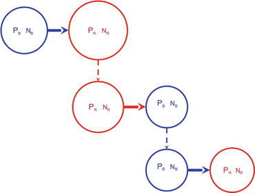
Lanchester’s model of combat is based upon simultaneous and continuous exchange of fire. In real combat, one side may often open fire before the other when it comes into a suitable range. This can confer an advantage if it achieves a large reduction in opposing force numbers before receiving counter fire [29]. In the game, the play is fixed turn sequence, which results in a sequential exchange of fire as shown below (Figure 3).

Figure 3.

Schematic representation of the Lanchester model for combat as a stochastic Markov chain, where fire exchange is sequential rather than simultaneous. The area of each circle is proportional to the number of troops N_B & N_R in each force. Note the steady reduction in numbers of troops for both Red and Blue forces due to attrition in combat, which is driven in part by stochastic dice rolls against fixed probabilities of hitting an opponent.

This can be described as a stochastic Markov Chain, where the next step in the game, in terms of combat outcome, depends on the state attained in the previous event with respect to fighting strength. To this extent, the fighting strength constantly changes turn by turn as numbers decline and ranges alter, which adjusts the probability of hitting an opponent. Consequently, players need to pay constant attention to the strategies for combat suggested in Table 1 as the game proceeds. Despite the differences highlighted above, MMW serves as a means of studying whether such a simple wargame follows aspects of the Lanchester model in an accessible form. Lanchester models are deterministic, and there is value in exploring deterministic models.

3. Example games to test Lanchester’s equations using MMW

3.1 Fighting strength vs. different troop levels, quality and combat range

Based on the probability outcomes for success in combat in the game with ranges as defined in Table 2, we can examine the fighting strength for a series of different troop levels (10, 12, 14, 16, and 20 units) and quality (poor, regular, good). These are tabulated below.

Number of troops; (−1 on dice roll)	1 hex	2 hexes	3 hexes	4 hexes	5 hexes	6 hexes
10 (−1)	83.3	66.7	50.0	33.3	16.7	0.0
12 (−1)	120.0	96.0	72.0	48.0	24.0	0.0
14 (−1)	163.3	130.7	98.0	65.3	32.7	0.0
16 (−1)	213.3	170.7	128.0	85.3	42.7	0.0
20 (−1)	333.3	266.7	200.0	133.3	66.7	0.0

Table 4.

Fighting strength (P N²) from probabilities of hitting vs. range in hexes and number of available poor quality troops. (−1) is added to all 1D6 casts, so the bottom row in Table 2 is used to calculate the fighting strength.

Number of troops (+1 on dice roll)	1 hex	2 hexes	3 hexes	4 hexes	5 hexes	6 hexes
10 (+1)	100.0	100.0	83.3	66.7	50.0	33.3
12 (+1)	144.0	144.0	120.0	96.0	72.0	48.0
14 (+1)	196.0	196.0	163.3	130.7	98.0	65.3
16 (+1)	256.0	256.0	213.3	170.7	128.0	85.3
20 (+1)	400.0	400.0	333.3	266.7	200.0	133.3

Table 5.

Fighting strength (P N²) from probabilities of hitting vs. range in hexes and number of available good quality troops. (+1) is added to all 1D6 casts, so the top row in Table 2 is used to calculate the fighting strength.

Number of troops (0 on dice roll)	1 hex	2 hexes	3 hexes	4 hexes	5 hexes	6 hexes
10 (0)	100.0	83.3	66.7	50.0	33.3	16.7
12 (0)	144.0	120.0	96.0	72.0	48.0	24.0
14 (0)	196.0	163.3	130.7	98.0	65.3	32.7
16 (0)	256.0	213.3	170.7	128.0	85.3	42.7
20 (0)	400.0	333.3	266.7	200.0	133.3	66.7

Table 6.

Fighting strength (P N²) from probabilities of hitting vs. range in hexes and number of available regular quality troops. (0) is added to all 1D6 casts, so the middle row in Table 2 is used to calculate the fighting strength.

Furthermore, closing the range has a large effect in improving fighting strength for both an attacker and a defender. Given the game plays with a fixed turn sequence (IgoYougo), an attacker must move into range before firing, necessarily exposing themselves to fire exchange before returning fire in the next turn. In this paper for all battles Red is the attacker advancing on Blue defending, generally resulting in Blue firing first from the turn sequence. This may give the Blue defender an inbuilt advantage and is a tactical consequence of the simple game rules not envisaged in Lanchester’s original work, which has continuous simultaneous firing. Nevertheless, MMW can examine pre-contact fighting strength (determined at the longest mutual range for fire exchange) and its ability to predict the winner in a battle. This is done in a series of asymmetrical games, which have different numbers of troops and troop quality to test whether values of pre-contact fighting strength are robust indicators of success or failure. Following this an examination of symmetrical pre-contact fighting strengths with troops of identical levels and quality is conducted, together with near symmetrical fighting strengths. Lanchester [1] stated in battles for equal fighting strength

In the case of equal forces the two conjugate curves become coincident; there is a single curve of logarithmic form; the battle is prolonged indefinitely. Since the forces actually consist of a finite number of finite units (instead of an infinite number of infinitesimal units), the end of the curve must show discontinuity, and break off abruptly when the last man is reached; the law based on averages evidently does not hold rigidly when the numbers become small. Beyond this, the condition of two equal curves is unstable, and any advantage secured by either side will tend to augment.

Lanchester’s equations indicate that forces with matched fighting strengths will eliminate each other, the consequence of an exchange of fire that is both deterministic and continuous, with a proviso that attrition may make one side gain numerical advantage towards the end of the combat. MMW has an exchange of fire that is sequential and stochastic, inevitably resulting in asymmetric numbers of forces evolving during the battle. If the forces have a matched probability of hitting in fire exchange then a difference in fighting strength can only arise from a reduction in numbers. Since the fighting strengths are matched and Lanchester’s model gives mutual reduction in forces under these conditions, two explanations in this wargame for eventual defeat by one side are offered.

1. For losses between forces initially stochastically matched, a tipping point will be likely reached when the number of units for one side reduces to 5, as seen from Figures 7 and 8 in Appendix B. Any further fall in unit numbers from 5 causes the probability of hitting to change by about 10% which is a large deleterious effect. If a force has greater than 5 units and the opponent falls to 5 or less, then it becomes increasingly unlikely that the disparity in forces can be reversed in the game. A number differential of at least 6 to 5 gives a difference of (6/5)² = 44% in fighting strengths, given the dependency on the square of the numbers concerned, indicating a likely win for the force with more units.

2. Alternatively the side that inflicts the first major losses on their opponent gains an advantage in fighting strength, and is likely to secure victory in the remainder of the fire exchange. This advantage can arise stochastically.

3.2 Asymmetric fighting strength games

In this section a test is made of fighting strength and whether it can predict the outcome of a battle ahead of first contact and subsequent fire exchange. Fighting efficiency is altered by troop quality at the longest range mutual fire exchange can occur and combining this with the number of troops this alters the fighting strength. Section 3.2.1 looks at a Red force that outnumbers a Blue force by 2:1 but with a disparity in troop quality, in a test of whether successive waves of attacks or a mass attack is more likely to win. Section 3.2.2 examines in a systematic manner using a designed-experiment approach the fighting strength based on fighting efficiency and numbers for a Red force employing varying tactics against a defensive Blue force with fixed numbers. This determines whether fighting strength is the key determinant, or whether tactics are also important. Section 3.2.3 uses a randomised sequence of fighting strengths by altering troop quality and numbers for both the Red and Blue forces, with both employing a steady firing line, again as a check of the importance of fighting strength as a battle outcome indicator. In all these battles a prediction of the eventual winner from the initial fighting strength and the % survivors predicted from Eq. (A11) is made and compared to the outcome.

3.2.1 Test of concentration of forces: single attack vs. waves

Three runs were conducted to demonstrate Lanchester’s concept of concentration of force for effective fighting. A force of 21 poor quality Red troops attack a force of defending 10 good quality Blue troops. In the first run 3 waves of 7 Red troops attack, spaced by 2 moves apart. In the second run 2 waves of 11 and 10 Red troops attack, spaced by 2 moves apart. In the third run a single wave of 21 Red troops attack. The results are below and shown graphically in [30] as animated gifs, together with a plot of % remaining units and fighting strengths per turn. The data in runs 1a-3, Table 12, Appendix C highlight the importance of attacking in strength, with the Red force defeated in runs 1 & 2, but overwhelming Blue in run 3 despite having the same number of Red units available in all runs. The battle prediction follows the expected pattern from the initial fighting strengths calculated, and in all further runs in this paper the Red force attacks in one wave.

3.2.2 Designed experiment

A previous study used a factorial designed experiment [31] on a simple wargame called ‘Take that Hill’ [32]. The study showed the advantage of this method in exploring games quickly and systematically. In this paper, 5 variables are examined using another type of experimental design [33] to test the effect of numbers vs. simple tactics for a Red force in an attacking role against a fixed number of Blue forces in a defensive role. The variables are set at low (−1) and high (+1) values. They include Red Force Tactics [Fire and manoeuvre, closing to (range) (+1) or Hit at (range) then retire regroup repeat (−1)], Red Force Attack Range {(max range in hexes − 2 (+1) or max range in hexes (−1)}, Red Force Attack Method {attacking nearest enemy regardless of fighting strength (+1), or attacking flank or weakest group (−1)], Red Force Trapdoor use {using trapdoors (+1) or not using trapdoors (−1)}, and finally Red Force Numbers (lower (−1) or higher (+1)}. In the case of fire and manoeuvre, the initial contact troops will begin firing at the enemy, then subsequent troops will join this firing line, allowing the surviving initial troops to rush forward by one hex and so on until the optimal firing distance by the attack range is reached. Previous work [34] indicated an effect on survivability in manoeuvre-and-fire combat to rush distance for an attacking force, so the value chosen in this game is representative of the rush distance suggested. The experimental pattern is shown in Table 7.

These can be used to produce scripted strategies for the Red force. In each game the initial fighting strengths, expected asymptote survival %, result, final survival %, and the game time in moves is tracked for analysis.

RunOrder	Red Force Tactics; A	Red Force; Attack Range; B	Red Force; Attack Method; C	Red Force; Trapdoors; D	Red Force Numbers; E
1	1	1	1	−1	−1
2	1	−1	−1	1	−1
3	−1	−1	−1	−1	−1
4	−1	1	−1	1	1
5	1	1	−1	−1	1
6	1	−1	1	1	1
7	−1	1	1	1	−1
8	−1	−1	1	−1	1

Table 7.

Designed experiment using 8 runs for 5 variables, labelled A–E (see Appendix B).

3.2.2.1 Red force with regular quality and 12 or 16 units vs. Blue force with good quality and 10 units

The matching numbers for a Red force of regular quality achieving balance in fighting strength from Eq. (A12) in Appendix A is 14.1 units against 10 Blue units of good quality. Careful selection of the Red force numbers around this saddle point of 14.1 units suggests 12 units for a low level and 16 units for a high level. The two values for Red force numbers straddle this value and so serve as a critical test of the influence of fighting strengths. The designed experiment in Table 7 then generates the following scripted attacking strategies for the Red force (Table 8).

Run	Scripted attacking Red force strategies
4	Manoeuvre and fire, closing to max range—2 attacking nearest group not using trapdoors with 12 units
5	Manoeuvre and fire, closing to max range attacking flank or weakest group using trapdoors with 12 units
6	Hit at max range attacking flank or weakest group then retire, regroup and repeat not using trapdoors with 12 units
7	Hit at max range—2 attacking flank or weakest group then retire, regroup and repeat using trapdoors with 16 units
8	Manoeuvre and fire, closing to max range—2 attacking flank or weakest group not using trapdoors with 16 units
9	Manoeuvre and fire, closing to max range attacking nearest group using trapdoors with 16 units
10	Hit at max range—2 attacking nearest group then retire, regroup and repeat using trapdoors with 12 units
11	Hit at max range attacking nearest group then retire, regroup and repeat not using trapdoors with 16 units

Table 8.

Scripted attacking Red force strategies in the trial shown in Table 13, Appendix C.

Number of troops (dice modifer)	1 hex	2 hexes	3 hexes	4 hexes	5 hexes	6 hexes
10 (+1)	100.0	100.0	83.3	66.7	50.0	33.3
12 (0)	144.0	120.0	96.0	72.0	48.0	24.0
16 (0)	256.0	213.3	170.7	128.0	85.3	42.7

Table 9.

Fighting strength vs. combat range for forces in the trial.

From the probabilities in Tables 4 and 5 the following relationships of fighting strength for an initial Blue force of 10 units, of good quality vs. two Red forces of 12 & 16, of regular quality are shown in Table 9.

Note that at the longest attack range of 6 hexes, a Blue force of 10 units is stronger than a Red force of 12 units, since P_R N_R² (24.0) < P_B N_B² (33.3). This advantage drops at an attack range of 4 hexes, when P_R N_R² (72.0) > P_B N_B² (66.7). This illustrates the effect of probability from combat range on fighting strength. It is clearly in Blue forces interest to keep Red force at arms length, but for a Red force to “Grab Their Belts to Fight Them!” and close the distance with the Blue force, accepting their losses on the way in. Consequently we might expect from fighting strength a force of 10 Blue units of good quality to beat a regular force of 12 Red units of regular quality at long range, but lose at shorter range, other things being equal. Also note that at the longest attack range of 6 hexes, a force of 10 Blue units at good quality is weaker than a force of 16 Red units at regular quality, since P_R N_R² (42.7) > P_B N_B² (33.3). This advantage increases at an attack range of 4 hexes, when P_R N_R² (128.0) ≫ P_B N_B² (66.7). Overall, we might anticipate a Blue force of 10 units of good quality can beat a Red force of 12 units of regular quality, but lose to a Red force of 16 units, also of regular quality. The games were played and all are available as animated gifs [30], together with plots of % remaining units and fighting strength turn by turn. The results are given in runs 4-11, Table 13, Appendix C.

In 8 out of 8 battles the initial fighting strength indicator based on long range combat correctly predicted the outcome of the battle, suggesting the identified saddle point in Red numbers by Eq. (A12) is real. Detailed analysis by best subsets regression analysis of each variable on the % survivors for each side, and number of moves until the end of the wargame is described in Appendix C. The most significant variable to explain the eventual outcome of each battle is the number of Red forces involved (E). In addition, all tactical effects (A–D) do influence the time for the battle to end in annihilation of one side.

3.2.2.2 Red force with poor quality and 16 or 20 units vs. Blue force with good quality and 10 units

The matching numbers for a Red force of poor quality achieving balance in fighting strength from Eq. (A12) is 17.3 units against 10 Blue units of good quality. Careful selection of the Red force numbers around the saddle point of 17.3 units suggests 16 units for a low level and 20 units for a high level. The two values for Red force numbers straddle this and so serve as a critical test of the fighting strengths.

The designed experiment in Table 7 generates the following scripted attacking strategies for the Red force (Table 10).

Run	Scripted attacking Red force strategies
12	Manoeuvre and fire, closing to max range—2 attacking nearest group not using trapdoors with 16 units
13	Manoeuvre and fire, closing to max range attacking flank or weakest group using trapdoors with 16 units
14	Hit at max range attacking flank or weakest group then retire, regroup and repeat not using trapdoors with 16 units
15	Hit at max range—2 attacking flank or weakest group then retire, regroup and repeat using trapdoors with 20 units
16	Manoeuvre and fire, closing to max range—2 attacking flank or weakest group not using trapdoors with 20 units
17	Manoeuvre and fire, closing to max range attacking nearest group using trapdoors with 20 units
18	Hit at max range—2 attacking nearest group then retire, regroup and repeat using trapdoors with 16 units
19	Hit at max range attacking nearest group then retire, regroup and repeat not using trapdoors with 20 units

Table 10.

Scripted attacking Red force strategies in the trial shown in Table 14, Appendix C.

Number of troops (dice modifer)	1 hex	2 hex	3 hex	4 hex	5 hex	6 hex
10 (+1)	100.0	100.0	83.3	66.7	50.0	33.3
16 (−1)	213.3	170.7	128.0	85.3	42.7	0.0
20 (−1)	333.3	266.7	200.0	133.3	66.7	0.0

Table 11.

Fighting strength vs. combat range for forces in the trial.

We note from Tables 4 and 6 the following relationships for an initial Blue force of 10, of good quality (+1 on 1D6 dice rolls) vs. two Red forces of 16 & 20, of poor quality (−1 on 1D6 dice rolls) (Table 11).

Note that at the longest attack range of 6 hexes, the Blue force is stronger than all Red forces, since Red cannot hit. At an attack range of 5 hexes, a force of 10 Blue units is stronger than a force of 16 Red units, since P_R N_R² (42.7) ≪ P_B N_B² (50.0). This advantage changes at an attack range of 4 hexes, when P_R N_R² (85.3) ≫ P_B N_B² (66.7). At the longest mutual attack range of 5 hexes, a force of 10 Blue units is weaker than a force of 20 Red units with poor quality, since P_R N_R² (66.7) ≫ P_B N_B² (50.0). This advantage to Red increases at an attack range of 4 hexes, when P_R N_R² (133.3) ≫ P_B N_B² (66.7). Consequently we might anticipate a Blue force of 10 units of good quality can beat a poor quality Red force of 16 units, but lose to a Red force of 20 units, unless they are able to keep the Red forces at a maximum firing range of 6 hexes.

The wargames were played and are available as animated gifs [30], together with the % surviving units and the fighting strengths, turn by turn. The outcomes are shown in runs 12-19 Table 14, Appendix C.

In 7 out of 8 battles the initial fighting strengths correctly predicted the outcome of the battle, again suggesting the identified saddle point in Red numbers by Eq. (A12) is real. Run 8 was incorrectly predicted. 10 Blue units fired on 20 Red units causing 5 hits at odds of hitting of 1/2. In return, 15 Red units fired but obtained no hits. At odds of success of 1/6, 15/6 = 2.5 hits might be deterministically expected, which would have reduced the Blue units significantly. However from Appendix B Eq. (A17), the odds of not hitting with 15 units each with a separate dice roll is 6.5%. Since this did not occur a second fire exchange from Blue caused a further 5 hits on Red. At this point the fighting strengths for 10 Red (16.7) vs. 10 Blue (50.0) indicated a Blue win, the eventual outcome. The predicted results based on initial fighting strengths are not deterministic, and this demonstration of the stochastic fire exchange in the game gives a probability of the estimated eventual outcome at 95% confidence for asymmetric battles.

Detailed analysis by best subsets regression analysis of the variables on the % survivors for each side, and number of moves until the end of the wargame is described in Appendix C. The most significant variable to explain the eventual outcome of each battle is the number of Red forces involved (E). In addition, tactical effects (A–D) do influence number of survivors and the time for the battle to end in annihilation of one side, especially variables A and B.

From the battles in Section 3.2, small differences in numbers combined with changes in probabilities produces different fighting strengths, and different end battle outcomes. Runs 7–9 and 11 had Red with 16 regular troops and a fighting strength of 42.3 against Blue with 10 good troops and a fighting strength of 33.3. In each battle the Red force annihilated the Blue force. Likewise, runs 12–14 and 18 had a Red force with 16 poor troops and a fighting strength of 42.7 against a Blue force with 10 good troops and a fighting strength of 50.0. In each battle the Blue force annihilated the Red force. Clearly the fighting strength appears to be a good indicator of success.

3.2.3 Randomised trials of asymmetric Red and Blue forces using steady firing line at max range

Fighting strengths listed in Tables 4 to 6 were studied by randomising troop numbers and quality for both Red and Blue forces. Each side was free to use their own tactics. This produced runs 20-34 in Table 15, Appendix C, together with their outcomes. This produced the following trial, together with their outcomes.

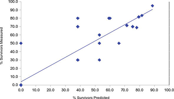
Across all the asymmetric battles in runs 1–34, the outcome was correctly predicted using the pre-contact fighting strength indicator for 33 out of 34 battles or 97%. Plotting the % survivors predicted from Eq. (A11) vs. % survivors measured is also instructive using the data in Tables 12 to 15.

The critical value of Pearson’s Correlation Coefficient at 99% confidence and 32 degrees of freedom (DoF) is 0.449. The two values for the correlation coefficient in Figures 4 and 5 exceed this, so the trends are significant at the 99% confidence level, implying the predictions in the game of winning or losing outcomes (by fighting strength) and the % survivors (by Lanchester’s Eq. (A11)) are reliable, probably at the 95% level, and the asymmetric battles in the game conform well to Lanchester’s expectations.

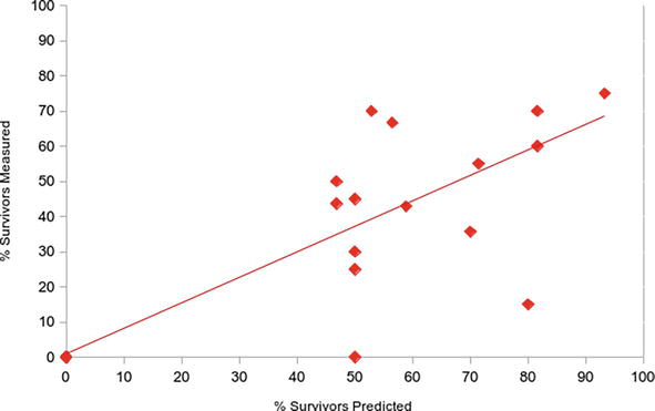
Figure 4.

% survivors predicted from Eq. (A11) vs. % survivors measured for Blue force from all runs from data in Tables 12 to 15. The slope, intercept and correlation coefficient for the data are m = 0.98, c = 4.08 and R = 0.91 (32 DoF) respectively.

Figure 5.

% survivors predicted from Eq. (A11) vs. % survivors measured for Red force from all runs from data in Tables 12 to 15. The slope, intercept and correlation coefficient for the data are m = 0.72, c = 1.09 and R = 0.86 (32 DoF).

3.3 Symmetrical fighting strength battles

3.3.1 Symmetrical fighting strength battles

Section 3.2 indicates that fighting strength is a good indicator for success in MMW. Real battles are rarely conducted between forces that exactly match each other in fighting strength. Hobby games tend to have symmetrically matched starting conditions in a sense of fairness between the players.

Runs [35–49] were fought between Red and Blue with matched fighting strengths based on equal troop quality to test the concepts of (a & b) in Section 3.1, with Red launching a central attack using a steady firing line against Blue in a trial of strength. This produced runs 35-49 given in Table 16, Appendix C, together with their outcomes.

The progress in each battle clearly shows stochastic behaviour in the fire exchange, and that explanation (a) in Section 3.1 appears to apply. Red won 6 of the battles with Blue winning 9 of the battles. This may indicate a slight bias towards the Blue defending force, especially when one considers the % remaining units left at the end of the battles. By this measure, when Red won their battles they had fewer % remaining units compared to the battles that Blue won. This gives some credence for explanation (b) in Section 3.1 also being present in the games.

3.3.2 Nearly symmetrical forces with closely matched fighting strengths

Saddle points where the fighting strengths between different numbers and troop qualities between Red and Blue have already been identified from Eq. (A12) and used in the asymmetric battles. In this section, values close to these were chosen for the Red forces producing 3 battles with nearly symmetrical fighting strengths. There is a slight imbalance in forces which from Lanchester’s equations should lead to the Blue Force winning each battle. This produced runs 50-52 given in Table 17, Appendix C, together with their outcomes.

Red won 1 of the battles with Blue winning 2 of the battles. Overall from the symmetric and nearly symmetric battles in Sections 3.3.1 and 3.3.2 there are 7 Red wins (avg % units remaining 38.5%), 11 Blue wins (avg % units remaining 70.2%). There is some evidence for defender bias (b) in these battles. There are also plenty of examples for exchange of fire leading to condition (a) in the runs. Stochastic behaviour in fire exchange leads to the balance of forces swinging to one side, and thereafter, Lanchester’s insights apply.

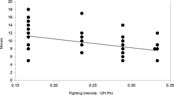
Taylor [35] introduced the concept of ‘fighting intensity’, $\sqrt{P_R\ast P_B}$ where P_B and P_B are the probabilities of hitting an opponent. Taking the probabilities for mutual fire exchange for Red and Blue from Table 2, calculating $\sqrt{P_R\ast P_B}$ and plotting against the number of moves for the battle to end for each of the runs in Tables 12–16 gives

The critical value of Pearson’s Correlation Coefficient at 99% confidence and 47 degrees of freedom (DoF) is 0.372, suggesting the trend is significant at the 99% confidence level. ‘fighting intensity’ is a guide for battle duration in MMW, with higher ‘fighting intensity’ i.e. improved odds in hitting reducing the number of moves to complete the battle (Figure 6).

Figure 6.

Moves for battle to end vs. ‘fighting intensity’ from all runs in Tables 3 and 12–16. The correlation coefficient for the data is R = −0.441 (47 DoF).

4. Conclusions

When is a battle lost? von Clausewitz [36] gives his own definition.

“The result of the whole combat consists in the sum total of the results of all partial combats; but these results of separate combats are settled by different considerations. First by the pure moral power in the mind of the leading officers. Secondly, by the quicker melting away of our troops, which can be easily estimated in the slow and relatively little tumultuary course of our battles. Thirdly, by lost ground.

Perhaps in battles that can be described by Lanchester’s equations the result is mostly a foregone conclusion if the Fighting Strengths are widely dissimilar before battle is joined. However Vernichtungsschlacht remains a Fata Morgana of the modern military experience [37].

There is a clear mismatch between the assumptions in Lanchester’s model and the simple manoeuvre and fire MMW, which uses sequential turns and stochastic exchange of fire. Despite these differences it appears that Lanchester’s concept of initial fighting strength $P{N}^2$ has some validity in predicting the outcomes in the study, with 33 out of 34 battles successfully predicted resulting in the Vernichtungsschlacht outcome. This suggests that the concept behind maximal fighting strength, namely a concentration of forces and their use in fire exchange to best advantage, firing first if possible, are key to success in MMW, as in real combat.

The battle outcomes from initial fighting strength at the longest mutual combat range predicted the final result 33 out of 34 times across the asymmetric runs. This indicates it is a good prognosis for eventual battle outcome. Note that neither explanation of (a) being reduced to 5 units or (b) inflicting first major losses appeared to apply for almost all the asymmetric battles, where victory went to the side at 95% confidence with fighting strength advantage, regardless of being Red or Blue, with the exception of run 19. In the symmetric games, once attrition swings the force balance to one side the fighting strength in combat is also a good prognosis for eventual battle outcome.

Military reality is more complex than either Lanchester’s model or a simple manoeuvre and fire wargame. Regarding Lanchester’s model, in addition to the variables in Table 11 the following are also neglected. The model considers homogeneous forces only. No replacements or manoeuvre to withdraw are possible. There is no consideration of non combat losses (e.g. surrenders, desertions). Suppressive effects of weapons rather than outright elimination are not considered. There are no logistical considerations. Effects of terrain or weather conditions are not considered. There are numerous academic papers which try to adapt Lanchester’s equations to reflect the subtlety of real combat, and the caveats with the model with some success which are listed in the references [35, 38, 39, 40, 41, 42, 43, 44, 45] for interested readers. Lanchester equations have been applied with success, primarily to idealised situations, given that they do not—nor do they try to—take into account fatigue, morale, or in-battle decision-making. The aim of a professional wargame is to address variables such as the above and include as many as desired in the rules and fighting maps used. It remains to be seen if the concept of fighting strength can be used to predict the outcomes of more sophisticated wargames.

Whether a simple or professional wargame, as in war itself, the Biblical warning from Luke still stands.

Or what king, going to make war against another king, sitteth not down first, and consulteth whether he be able with ten thousand to meet him that cometh against him with twenty thousand? Luke 14:31.

Appendix A. Lanchester’s equations

Quoting directly from Lanchester’s original work [1].

“If, again, we assume equal individual fighting value, and the combatants otherwise on terms of equality, each man will in a given time score, on an average, a certain number of hits that are effective; consequently, the number of men knocked out per unit time will be directly proportional to the numerical strength of the opposing force.”

We now prove this statement. Suppose we have two forces in combat, Red and Blue, who allocate fire to a new target when a previous one is hit and eliminated from further action. The original numbers of Red and Blue forces are N_R and N_B. The ‘efficiency’ or probability of hitting an opponent in a fire exchange, removing them from further combat, is P_R for Red and P_B for Blue forces.

If we assume simultaneous and continuous exchange of fire the rate of Red forces losses is

$$\frac{{\mathit{dN}}_R}{\mathit{dt}}=-P_B{N}_B$$A1

and the rate of Blue force losses is

$$\frac{{\mathit{dN}}_B}{\mathit{dt}}=-P_R{N}_R$$A2

Define the fighting strength F by the equation:

$$P{N}^2$$A3

and consider the difference, S, in the fighting strengths between the two forces:

$$S=P_R{N}_R^2-P_B{N}_B^2$$A4

Differentiate this with respect to time, to obtain:

$$\frac{\mathit{dS}}{\mathit{dt}}=2\left[P_R{N}_R\frac{{\mathit{dN}}_R}{\mathit{dt}}-P_B{N}_B\frac{{\mathit{dN}}_B}{\mathit{dt}}\right]$$A5

Now substitute in the time derivatives in [A2] and [A3] to see:

$$\frac{\mathit{dS}}{\mathit{dt}}=2\left[P_R{N}_R\frac{{\mathit{dN}}_R}{\mathit{dt}}-P_B{N}_B\frac{{\mathit{dN}}_B}{\mathit{dt}}\right]=2\left[P_R{N}_R\left(-P_B{N}_B\right)+P_B{N}_B{P}_R{N}_R\right]=0$$A6

This means that the difference in the fighting strengths between the two forces does not change during the battle. Mathematically, this means:

$$P_R{N}_R^2\left(t\right)-P_B{N}_B^2\left(t\right)=\mathit{\text{constant}}$$A7

Apply this formal at two times. The first, at the opening of the conflict and time t = 0, the second at the end of the conflict, when t = T. We assume that at the end, the Blue forces have been annihilated, which will occur if $P_R{N}_R^2>P_B{N}_B^2$. As a consequence:

$$P_R{N}_R^2\left(T\right)=P_R{N}_R^2\left(0\right)-P_B{N}_B^2\left(0\right)$$A8

Divide through by $P_R$ to obtain:

$$N_R^2\left(T\right)=N_R^2\left(0\right)-\frac{P_B}{P_R}{N}_B^2\left(0\right)$$A9

So that:

$$N_R^2\left(T\right)=N_R^2\left(0\right)\left[1-\frac{P_B{N}_B^2\left(0\right)}{P_R{N}_R^2\left(0\right)}\right]$$A10

Or equivalently:

$$N_R\left(T\right)=N_R\left(0\right)\sqrt{1-\frac{P_B{N}_B^2\left(0\right)}{P_R{N}_R^2\left(0\right)}}$$A11

Consequently, the number of Red forces remaining at the end of the conflict depends on both the initial number of Red forces, but also on the ratio of the fighting strengths of the Blue to Red forces. The greater the fighting strength of the Blue forces, the more losses the Red forces will suffer.

If the initial fighting strength for the Red Force is less than the Blue Force, then $P_R{N}_R^2\left(0\right)<P_B{N}_B^2\left(0\right)$, and the Red force will lose the battle and be annihilated. Eq. (A11) will predict the number of Blue survivors under these conditions if we interchange the Red and Blue subscripts.

In the case of ‘symmetrical’ matched fighting strengths at the start of fire exchange between Red and Blue forces $P_R{N}_R^2\left(0\right)=P_B{N}_B^2\left(0\right)$. Examining this gives the adjustments needed to the starting ‘asymmetrical’ unmatched fighting strengths to make them ‘symmetrical’ matched fighting strengths:

$$\text{For initial force numbers}{N}_R\left(0\right)=N_B\sqrt{\left(\frac{P_B}{P_R}\right)}$$A12

$$\text{For effectiveness}{P}_R\left(0\right)=N_B\left(0\right){\left(\frac{P_B}{P_R}\right)}^2$$A13

Eqs. (A12) and (A13) predict the numbers for the Blue force if we interchange the Red and Blue subscripts.

Taylor [35] gives a solution for the time to annihilation in Lanchester’s model, but this does not apply in this study due to the different time dependence of sequential play of the wargame used. Further details on the theory and extensions therein can be found in the following papers [38, 39, 40, 41, 42, 43, 44, 45].

B. Probability of rolling a target value in repeated 1D6 casts

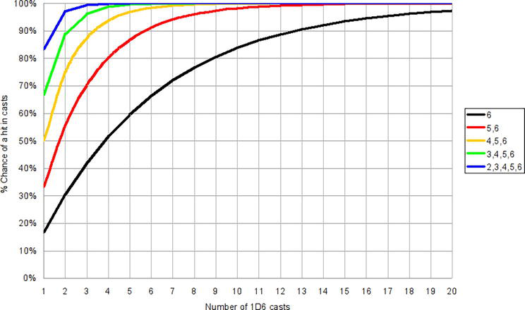
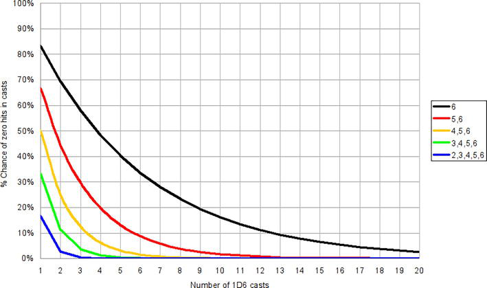
Define the number of faces, f, on a 1D6 that yields the desired outcome for a hit from rolling 1D6 n times. The chances of rolling the required value, f, in repeated n casts of 1D6 is

$$1-{\left(\frac{\left(6-f\right)}{6}\right)}^n$$A14

Likewise the chances of not rolling the required value, f, in repeated n casts of 1D6 is

$${\left(\frac{\left(6-f\right)}{6}\right)}^n$$A15

By example the chance of rolling a six (f = 1) in 15 casts is

$$1-{\left(\frac{\left(6-1\right)}{6}\right)}^{15}=0.935$$A16

And the chance of not rolling a six (f = 1) in 15 casts is

$${\left(\frac{\left(6-1\right)}{6}\right)}^n=0.065$$A17

In the game, the probability needed to hit changes with quality and range as shown in Table 2. For regular quality units at six hexes, a 6 is required (f = 1) to hit. At 5 hexes a cast of 5 or 6 is required (f = 2) to hit. At 4 hexes a cast of 4, 5 or 6 is required (f = 3) to hit. Taking (A14) and (A15) and plotting them against 20 1D6 rolls vs. target scores (2–6 to 6) gives

Note the shape of change in probability with number of casts and target value for a hit to occur. As hits accrue to a force the number of units that can fire reduces which translates to moving along the LHS of each curve. Changing the range translates to jumping between curves.

Figure 7.

Chance of a single hit from increasing 1D6 casts from Eq. (A14) vs. target scores.

Figure 8.

Chance of not achieving a single hit from increasing 1D6 casts from Eq. (A15) vs. target scores.

C. Table of results: predicted vs measured battle outcomes to test concentration of forces using Lanchester’s Equations

Run	Red	Blue	Fighting strengths (Red to Blue)	Prediction	% Survivors predicted (Red to Blue)	Outcome	% Survivors measured (Red to Blue)	Moves
1a	7 (−1)	10 (+1)	8.2 < 50.0	Blue win	0.0% & 91.5%	Blue win	0.0% & 80.0%	—
1b	7 (−1)	10 (+1)	8.2 < 50.0	Blue win	0.0% & 82.3%	Blue win	0.0% & 70.0%	—
1c	7 (−1)	10 (+1)	8.2 < 50.0	Blue win	0.0% & 75.3%	Blue win	0% & 70.0%	11
2a	11(−1)	10 (+1)	20.2 < 50.0	Blue win	0.0% & 77.2%	Blue win	0.0% & 80.0%	—
2b	10 (−1)	10 (+1)	16.7 < 50.0	Blue win	0.0% & 62.9%	Blue win	0.0% & 80.0%	9
3	21 (−1)	10 (+1)	73.3 > 50.0	Red win	56.5% & 0.0%	Red win	66.7% & 0.0%	8

Table 12.

Predicted vs. measured battle outcomes to test concentration of forces in an asymmetric battle between Blue and Red attacking in waves.

Run	Red	Blue	Fighting strengths (Red to Blue)	Prediction	% Survivors predicted (Red to Blue)	Outcome	% Survivors measured (Red to Blue)	Moves
4	12 (0)	10 (+1)	24.0 < 33.3	Blue win	0.0% & 52.9%	Blue win	0.0% & 50.0%	7
5	12 (0)	10 (+1)	24.0 < 33.3	Blue win	0.0% & 52.9%	Blue win	0.0% & 30.0%	12
6	12 (0)	10 (+1)	24.0 < 33.3	Blue win	0.0% & 52.9%	Blue win	0.0% & 60.0%	17
7	16 (0)	10 (+1)	42.3 > 33.3	Red win	46.8% & 0.0%	Red win	50.0% & 0.0%	10
8	16 (0)	10 (+1)	42.3 > 33.3	Red win	46.8% & 0.0%	Red win	50.0% & 0.0%	9
9	16 (0)	10 (+1)	42.3 > 33.3	Red win	46.8% & 0.0%	Red win	50.0% & 0.0%	7
10	12 (0)	10 (+1)	24.0 < 33.3	Blue win	0.0% & 52.9%	Blue win	0.0% & 60.0%	9
11	16 (0)	10 (+1)	42.3 > 33.3	Red win	46.8% & 0.0%	Red win	43.7% & 0.0%	11

Table 13.

Predicted vs. measured battle outcomes for the scripted strategy runs for a Blue force of 10 units of good quality vs. two Red forces of 12 & 16, of regular quality. The fighting strength assumes contact at 6 hexes, i.e. maximum mutual range.

Run	Red	Blue	Fighting strengths (Red to Blue)	Prediction	% Survivors predicted (Red to Blue)	Outcome	% Survivors measured (Red to Blue)	Moves
12	16 (−1)	10 (+1)	42.7 < 50.0	Blue win	0.0% & 38.3%	Blue win	0.0% & 70.0%	7
13	16 (−1)	10 (+1)	42.7 < 50.0	Blue win	0.0% & 38.3%	Blue win	0.0% & 30.0%	10
14	16 (−1)	10 (+1)	42.7 < 50.0	Blue win	0.0% & 38.3%	Blue win	0.0% & 80.0%	8
15	20 (−1)	10 (+1)	66.7 > 50.0	Red win	50.0% & 0.0%	Red win	25.0% & 0.0%	8
16	20 (−1)	10 (+1)	66.7 > 50.0	Red win	50.0% & 0.0%	Red win	45.0% & 0.0%	10
17	20 (−1)	10 (+1)	66.7 > 50.0	Red win	50.0% & 0.0%	Red win	30.0% & 0.0%	9
18	16 (−1)	10 (+1)	42.7 < 50.0	Blue win	0.0% & 38.3%	Blue win	0.0% & 30.0%	7
19	20 (−1)	10 (+1)	66.7 > 50.0	Red win	50.0% & 0.0%	Blue win	0.0% & 50.0%	14

Table 14.

Predicted vs. measured battle outcomes for the scripted strategy runs for a Blue force of 10 units of good quality vs. two Red forces of 16 & 20, of poor quality. The fighting strength assumes contact at 5 hexes, i.e. maximum mutual range.

Run	Red	Blue	Fighting strengths (Red to Blue)	Prediction	% Survivors predicted (Red to Blue)	Outcome	% Survivors measured (Red to Blue)	Moves
20	12 (+1)	16 (+1)	48.0 < 85.3	Blue win	0.0% & 66.1%	Blue win	0.0% & 50.0%	8
21	14 (−1)	12 (+1)	32.7 < 72.0	Blue win	0.0% & 81.6%	Blue win	0.0% & 83.3%	7
22	12 (−1)	14 (0)	24.0 < 65.3	Blue win	0.0% & 79.5%	Blue win	0.0% & 81.7%	7
23	10 (+1)	10 (−1)	50.0 > 16.7	Red win	81.6% & 0.0%	Red win	60.0% & 0.0%	6
24	20 (+1)	20 (−1)	200.0 > 66.7	Red win	81.6% & 0.0%	Red win	70.0% & 0.0%	6
25	16 (0)	20 (0)	42.7 < 66.7	Blue win	0.0% & 60.0%	Blue win	0.0% & 80.0%	13
26	10 (0)	12 (−1)	33.3 > 24.0	Red win	52.9% & 0.0%	Red win	70.0% & 0.0%	8
27	14 (+1)	16 (0)	65.3 > 42.7	Red win	58.9% & 0.0%	Red win	42.9% & 0.0%	11
28	16 (−1)	20 (+1)	42.7 < 200.0	Blue win	0.0% & 88.7%	Blue win	0.0% & 95.0%	5
29	20 (−1)	14 (−1)	66.7 > 32.7	Red win	71.4% & 0.0%	Red win	55.0% & 0.0%	11
30	10 (−1)	16 (−1)	16.7 < 42.7	Blue win	0.0% & 78.1%	Blue win	0.0% & 68.8%	5
31	12 (0)	14 (+1)	24.0 < 65.3	Blue win	0.0% & 71.4%	Blue win	0.0% & 71.4%	7
32	16 (+1)	10 (+1)	78.1 > 33.3	Red win	93.3% & 0.0%	Red win	75.0% & 0.0%	12
33	20 (0)	12 (0)	66.7 > 24.0	Red win	80.0% & 0.0%	Red win	15.0% & 0.0%	18
34	14 (0)	10 (0)	32.7 > 16.7	Red win	70.0% & 0.0%	Red win	35.7% & 0.0%	16

Table 15.

Predicted vs. measured battle outcomes for the asymmetric battles between Blue and Red forces of 10–20 units with poor to good quality. The fighting strength assumes fire exchange at maximum mutual range.

Run	Red	Blue	Fighting strengths (Red to Blue)	Prediction	% Survivors predicted (Red to Blue)	Outcome	% Survivors measured (Red to Blue)	Moves
35	10 (−1)	10 (−1)	16.7 = 16.7	Draw	0.0% & 0.0%	Red win	40.0% & 0.0%	15
36	10 (0)	10 (0)	16.7 = 16.7	Draw	0.0% & 0.0%	Red win	30.0% & 0.0%	12
37	10 (+1)	10 (+1)	33.3 = 33.3	Draw	0.0% & 0.0%	Blue win	0.0% & 80.0%	8
38	12 (−1)	12 (−1)	24.0 = 24.0	Draw	0.0% & 0.0%	Red win	58.3% & 0.0%	8
39	12 (0)	12 (0)	24.0 = 24.0	Draw	0.0% & 0.0%	Blue win	0.0% & 75.0%	9
40	12 (+1)	12 (+1)	48.0 = 48.0	Draw	0.0% & 0.0%	Blue win	0.0% & 91.7%	5
41	14 (−1)	14 (−1)	32.7 = 32.7	Draw	0.0% & 0.0%	Red win	57.1% & 0.0%	9
42	14 (0)	14 (0)	32.7 = 32.7	Draw	0.0% & 0.0%	Blue win	0.0% & 78.6%	9
43	14 (+1)	14 (+1)	65.3 = 65.3	Draw	0.0% & 0.0%	Red win	14.3% & 0.0%	9
44	16 (−1)	16 (−1)	42.7 = 42.7	Draw	0.0% & 0.0%	Red win	31.3% & 0.0%	14
45	16 (0)	16 (0)	42.7 = 42.7	Draw	0.0% & 0.0%	Blue win	0.0% & 62.5%	12
46	16 (+1)	16 (+1)	85.3 = 85.3	Draw	0.0% & 0.0%	Blue win	0.0% & 68.8%	5
47	20 (−1)	20 (−1)	66.7 = 66.7	Draw	0.0% & 0.0%	Blue win	0.0% & 45.0%	11
48	20 (0)	20 (0)	66.7 = 66.7	Draw	0.0% & 0.0%	Blue win	0.0% & 75.0%	12
49	20 (+1)	20 (+1)	133.3 = 133.3	Draw	0.0% & 0.0%	Blue win	0.0% & 55.0%	9

Table 16.

Predicted vs. measured battle outcomes for symmetric battles between Blue and Red forces of 10–20 units with regular quality. The fighting strength assumes contact at maximum mutual range depending on troop quality.

Run	Red	Blue	Fighting strengths (Red to Blue)	Prediction	% Survivors predicted (Red to Blue)	Outcome	% Survivors measured (Red to Blue)	Moves
50	7 (0)	10 (−1)	16.3 ≈ 16.7	Blue win	0.0% & 14.2%	Blue win	0.0% & 30.0%	10
51	14 (−1)	10 (0)	32.7 ≈ 33.0	Blue win	0.0% & 14.0%	Red win	42.9% & 0.0%	9
52	17 (−1)	10 (+1)	48.2 ≈ 50.0	Blue win	0.0% & 19.1%	Blue win	0.0% & 50.0%	8

Table 17.

Predicted vs. measured battle outcomes for nearly symmetrical battles between Blue and Red forces of 7–17 units with varying quality. The fighting strength assumes contact at maximum mutual range depending on troop quality.

D. Designed experiment analysis

The statistical methodology for analysing designed experiments is described in [30]. The designed experiment followed the pattern given in Table 4.

Best subsets regression analysis and regression equations were performed using Minitab v18 with +1, −1 for each variable shown in Table 4, together with the data in Tables 8 and 17. The variables were Red Force Tactics (A), Red Force Attack Range (B), Red Force Attack Method (C), Red Force using Trapdoors (D) and Red Force Numbers (E), with each variable set to −1 or +1 as described in Table 4. The responses studied were % Blue and Red remaining forces, and the time in moves for the wargame to end with the annihilation of one side.

D.1 Red force with regular quality and 12 or 16 units vs. Blue force with good quality and 10 units

Best subsets regression and regression equations identified were

See Tables 18–20.

Var	R-sq	Ad. R-sq	C-p	s	A	B	C	D	E
1	89.3	87.5	0.8	10.0					X
1	3.6	0.0	39.2	30.0	X
2	92.9	90.0	1.2	8.9	X				X
2	90.2	86.2	2.4	10.5		X			X
3	93.7	89.1	2.8	9.4	X	X			X
3	93.7	89.1	2.8	9.4	X		X		X
4	94.6	87.5	4.4	10.0	X	X	X		X
4	94.6	87.5	4.4	10.0	X	X		X	X
5	95.5	84.4	6.0	11.2	X	X	X	X	X

Table 18.

Blue % remaining: best subsets regression (best fit in bold text).

Var	R-sq	Ad. R-sq	C-p	s	A	B	C	D	E
1	99.4	99.3	2.0	2.2					X
1	0.1	0.0	946.3	28.0				X
2	99.5	99.3	3.0	2.2	X				X
2	99.5	99.3	3.0	2.2			X		X
3	99.6	99.3	4.0	2.2	X		X		X
3	99.6	99.3	4.0	2.2			X	X	X
4	99.7	99.3	5.0	2.2	X		X	X	X
4	99.7	99.3	5.0	2.2	X	X	X		X
5	99.8	99.3	6.0	2.2	X	X	X	X	X

Table 19.

Red % remaining: best subsets regression (best fit in bold text).

Var	R-sq	Ad. R-sq	C-p	s	A	B	C	D	E
1	33.3	22.2	192.0	2.9	X		X
1	24.5	41.0	122.0	2.5		X
2	57.8	41.0	122.0	2.5	X		X
2	57.8	41.0	122.0	2.5		X	X
3	82.3	69.0	52.0	1.8	X	X	X
3	68.7	45.2	92.0	2.4		X	X		X
4	93.2	84.1	22.0	1.3	X	X	X		X
4	88.4	73.0	36.0	1.7	X	X	X	X
5	99.3	97.6	6.0	0.5	X	X	X	X	X

Table 20.

Moves until end of wargame: best subsets regression (best fit in bold text).

i.e. only the number of Red troops mattered, and is independent of tactics.

The regression equation is

$$\%\text{Blue remaining}=25.0–25.0^{\ast }\mathrm{E}$$A18

i.e. only the number of Red troops mattered, and is independent of tactics.

The regression equation is

$$\%\mathrm{Red}\text{remaining}=24.2+24.2^{\ast }\mathrm{E}$$A19

i.e. all variables matter, and tactics plays a role.

The regression equation is

$$\text{Moves}=10.3–{1.50}^{\ast }\mathrm{A}–{1.50}^{\ast }\mathrm{B}–{1.75}^{\ast }\mathrm{C}–{0.750}^{\ast }\mathrm{D}–{1.00}^{\ast }\mathrm{E}$$A20

All variables have an effect, including the tactical ones. The shortest battle duration will happen when all variables are set to high values i.e. Fire and manoeuvre, closing to (range defined by force attack), Force Attack Range at (max range in hexes—2), Red Force Attack Method, attacking nearest enemy regardless of fighting strength, Red Force Attack Method, attacking nearest enemy regardless of fighting strength, Red Force Trapdoor use, using trapdoors, and Red Force Numbers set to higher levels.

D.2 Red force with regular quality and 12 or 20 units vs. Blue force with good quality and 10 units

Best subsets regression and regression equations identified were

See Tables 21–23.

Var	R-sq	Ad. R-sq	C-p	s	A	B	C	D	E
1	44.8	5.5	15.8	25.7					X
1	34.3	23.3	19.5	27.9				X
2	79.0	70.6	5.5	17.3				X	X
2	51.0	31.5	15.5	26.5	X				X
3	85.3	74.3	5.3	16.2		X		X	X
3	85.2	74.3	5.3	16.2	X		X		X
4	91.6	80.4	5.0	14.1	X	X		X	X
4	88.1	72.3	6.2	16.8	X		X	X	X
5	94.4	80.4	6.0	14.1	X	X	X	X	X

Table 21.

Blue % remaining: best subsets regression (best fit in bold text).

Var	R-sq	Ad. R-sq	C-p	s	A	B	C	D	E
1	54.3	46.7	2.5	13.23					X
1	13.6	0.0	0.0	18.2	X
2	67.9	55.1	2.5	12.15	X				X
2	63	48.3	3.2	13.04			X		X
3	76.6	59.1	3.3	11.59	X	X			X
3	76.6	59.1	3.3	11.59	X	X	X		X
4	85.3	65.8	4.1	10.61	X	X	X		X
4	77.2	46.7	5.2	13.23	X		X	X	X
5	85.9	50.5	6	12.75	X	X	X	X	X

Table 22.

Red % remaining: best subsets regression (best fit in bold text).

Var	R-sq	Ad. R-sq	C-p	s	A	B	C	D	E
1	27.5	15.4	0.0	2.1					X
1	27.5	15.4	0.0	2.1		X			X
2	54.9	36.9	0.5	1.8		X			X
2	35.9	10.3	1.6	2.2				X	X
3	63.4	35.9	2.0	1.8		X		X	X
3	55.3	21.7	2.5	2.0	X	X			X
4	63.9	15.4	4.0	2.1		X	X	X	X
4	63.7	15.4	4.0	2.1	X	X		X	X
5	64.1	0.0	6.0	2.6	X	X		X	X

Table 23.

Moves until end of wargame: best subsets regression (best fit in bold text).

i.e. only variables A, B, D and E, the number of Red troops mattered, and tactics (A, B, D) do matter.

The regression equation is

$$\%\text{Blue remaining}=32.5–7.{50}^{\ast }\mathrm{A}-7.{50}^{\ast }\mathrm{B}-17.5^{\ast }\mathrm{D}-20.0^{\ast }\mathrm{E}$$A21

i.e. only variables A, B, C and E the number of Red troops mattered, and tactics (A–C) do matter.

The regression equation is

$$\%\mathrm{Red}\text{remaining}=12.5+{6.25}^{\ast }\mathrm{A}+{5.00}^{\ast }\mathrm{B}-{5.00}^{\ast }\mathrm{C}+{12.5}^{\ast }\mathrm{E}$$A22

i.e. all variables matter, and tactics plays a role.

The regression equation is

$$\text{Moves}=9.13–{1.12}^{\ast }\mathrm{B}–{0.625}^{\ast }\mathrm{D}+{1.13}^{\ast }\mathrm{E}$$A23

Overall all variables matter, with the number of Red units the most significant. Tactics plays a role in time for a battle to conclude and also in the second designed experiment for % troops remaining. This highlights the weakness of tactical choice A at a negative value (hit at (range) then retire, regroup, and repeat) in the game. This exposes Red to Blue counterfire three times for every time it fires in return (once when closing to distance, once when counterfiring and once when Blue returns fire before retiring, then regrouping and repeating the process again).

References

1.Lanchester FW. The principle of concentration: N- square law, Chapter 5. In: Aircraft in Warfare: The Dawn of the Fourth Arm. London: Constable; 1916. Available from: https://tinyurl.com/3h9j63xv
2.Chan P. The Lanchester square law: Its implications for force structure and force preparation of Singapore’s operationally-ready soldiers’ pointer. Journal of Singapore Armed Forces;42(2):42-60. Available from: https://tinyurl.com/2k3sx868
3.Kingman JFC. Stochastic aspects of Lanchester’s theory of warfare. Journal of Applied Probability. 2002;39(3):455-465. Available from: http://www.jstor.com/stable/3216070
4.McCue B. Lanchester and the Battle of Trafalgar. Phalanx. 1999;32(4):10-13, 22. Available from: https://www.jstor.org/stable/43962654
5.Nash DH. Differential equations and the Battle of Trafalgar. The College Mathematics Journal. 1985;16(2):98-102. Available from: http://www.jstor.com/stable/2686209
6.MacKay N, Price C, Wood J. Weighing the fog of war: Illustrating the power of Bayesian methods for historical analysis through the Battle of the Dogger Bank. Historical Methods. 2016;49(2):80-91. DOI: 10.1080/01615440.2015.1072071
7.MacKay N, Price C, Wood J. Weight of Shell must tell: A Lanchestrian reappraisal of the Battle of Jutland. History. 2016;101(347):536-563. DOI: 10.1111/1468-229X.12241
8.Taylor TC. A simple, functional model of modern naval conflict. Naval War College Review. 1995;48(3):99-112. Available from: http://www.jstor.com/stable/44642811
9.Bongers A, Torres JL. Revisiting the Battle of midway. Military Operations Research. 2020;25(2):49-68. Available from: https://www.jstor.org/stable/10.2307/26917214
10.Armstrong MJ. The salvo combat model with a sequential exchange of fire. The Journal of the Operational Research Society. 2014;65(10):1593-1601. Available from: http://www.jstor.com/stable/24505020
11.Weiss HK. Combat models and historical data: The U.S. civil war. Operations Research. 1966;14(5):759-790. Available from: http://www.jstor.com/stable/168777
12.Johnson RL. Lanchester’s Square Law in Theory and Practice, AD-A225-484. Army Command and General Staff College Fort Leavenworth; 1989. Available from: https://apps.dtic.mil/sti/pdfs/ADA225484.pdf
13.Lucas TW, Dinges JA. The effect of Battle circumstances on fitting Lanchester equations to the Battle of Kursk. Military Operations Research. 2004;9(2):17-30. Available from: http://www.jstor.com/stable/43940971
14.Lucas TW. Fitting Lanchester equations to the battles of Kursk and Ardennes. Naval Research Logistics. 2004;51:95-116. DOI: 10.1002/nav.10101
15.Speight LR. Within-campaign analysis: A statistical evaluation of the Battle of Kursk. Military Operations Research. 2011;16(2):41-62. Available from: http://www.jstor.com/stable/43941475
16.Kuikka V. A combat equation derived from stochastic modeling of attrition data. Military Operations Research. 2015;20(3):49-69. Available from: https://www.jstor.org/stable/10.2307/24838621
17.Engel JH. A verification of Lanchester’s Law. Journal of the Operations Research Society of America. 1954;2(2):163-171. Available from: http://www.jstor.com/stable/166602
18.Schaffer MB. Lanchester models of guerrilla engagements. Operations Research. 1968;16(3):457-488. Available from: http://www.jstor.com/stable/168576
19.Kress M, Szechtman R. Why defeating insurgencies is hard: The effect of intelligence in counterinsurgency operations—A best-case scenario. Operations Research. 2009;57(3):578-585. Available from: http://www.jstor.com/stable/25614776
20.Atkinson MP, Gutfraind A, Kress M. When do armed revolts succeed: Lessons from Lanchester theory. Journal of the Operational Research Society. 2012;63(10):1363-1373. Available from: http://www.jstor.com/stable/41680007
21.MacKay NJ. When Lanchester met Richardson, the outcome was stalemate: A parable for mathematical models of insurgency. Journal of the Operational Research Society. 2015;66(2):191-201. Available from: http://www.jstor.com/stable/24505286
22.Kress M. Lanchester models for irregular warfare. Mathematics. 2020;8:737. DOI: 10.3390/math8050737
23.MacKay N, Price C. Safety in numbers: Ideas of concentration in Royal air Force Fighter Defence from Lanchester to the Battle of Britain. History. 2011;96(3):304-325. Available from: http://www.jstor.com/stable/24429278
24.Adams ES, Mesterton-Gibbons M. Lanchester’s attrition models and fights among social animals. Behavioral Ecology. 2003;14(5):719-723. DOI: 10.1093/beheco/arg061
25.Plowes NJR, Adams ES. An empirical test of Lanchester’s square law: Mortality during battles of the fire ant Solenopsis invicta. Proceedings: Biological Sciences. 2005, 2005;272(1574):1809-1814. Available from: http://www.jstor.com/stable/30047764
26.Möbius strip. Wikipedia. Available from: https://tinyurl.com/3jrs2xvt
27.Möbius mayhem 2123 - 'Vernichtungsschlacht' in the vacuum of space. Wargames Vault. 2023. Available from: https://tinyurl.com/mu7bp4en The game is free
28.Flanagan M, Lipscombe TC, Northey A, Robinson IM. Chance all—A simple 3D6 dice stopping game to explore probability and risk vs reward. London, UK, Intechopen: Game Theory—From Idea to Practice; 2022. Available from: https://www.intechopen.com/chapters/83376
29.Armstrong MJ. The salvo combat model with a sequential exchange of fire. Journal of the Operational Research Society. 2014;65(10):1593-1601. Available from: http://www.jstor.com/stable/24505020
30.Online gifs of games in Section 3. Available from: https://iactaaleaest.wordpress.com/2003/01/17/lanchesters-fighting-strength-as-a-battle-outcome-predictor-applied-to-a-simple-fire-and-manoeuvre-wargame-supporting-gifs/
31.Flanagan M, Northey A, Robinson IM. Exploring tactical choices and game design outcomes in a simple wargame ‘take that hill’ by a systematic approach using experimental design. International Journal of Serious Games. 2020;7(4):27-50. DOI: 10.17083/ijsg.v7i4.372
32.Take that Hill! UK Fight Club’s First Manual Wargame Primer. Available from: https://www.ukfightclub.co.uk/take-that-hill
33.Plackett RL, Burman JP. The design of optimum multifactorial experiments. Biometrika. 1946;33(4):305-325. DOI: 10.1093/biomet/33.4.305
34.Christy DE. A Lanchester Based Model for Analyzing Infantry Fire and Maneuver Tactics [M.S. in Operations Research]. Naval Postgraduate School; 1969. Available from: http://hdl.handle.net/10945/12536
35.Taylor JG. Lanchester-Type Models of Warfare. Volume I. Naval Postgraduate School. 1980. ADA090842. Available from: https://apps.dtic.mil/sti/pdfs/ADA090842.pdf
36.von Clausewitz C. Book 4, Chapter 4. In: On War. 1832. Available from: https://tinyurl.com/2p9hc78z
37.Battle of annihilation. Wikipedia. Available from: https://tinyurl.com/yjw57u92
38.Dolanský L. Present state of the Lanchester theory of combat. Operations Research. 1964;12(2):344-358 Available from: http://www.jstor.com/stable/167934
39.Anderton CH. Toward a mathematical theory of the offensive/defensive balance. International Studies Quarterly. 1992;36(1):75-99. Available from: http://www.jstor.com/stable/2600917
40.Kuikka V. A combat equation derived from stochastic modeling of attrition data. Military Operations Research. 2015;20(3):49-69. Available from: https://www.jstor.org/stable/10.2307/24838621
41.Taylor JG. Optimal commitment of forces in some Lanchester-type combat models. Operations Research. 1979;27(1):96-114. Available from: http://www.jstor.com/stable/170246
42.Kingman JFC. Stochastic aspects of Lanchester’s theory of warfare. Journal of Applied Probability. 2002;39(3):455-465. Available from: http://www.jstor.com/stable/3216070
43.Brooks FC. The stochastic properties of large Battle models. Operations Research. 1965;13(1):1-17. Available from: http://www.jstor.com/stable/167950
44.Brown RH. Theory of combat: The probability of winning. Operations Research. 1963;11(3):418-425. Available from: http://www.jstor.com/stable/168029
45.Brackney H. The dynamics of military combat. Operations Research. 1959;7(1):30-44. Available from: https://www.jstor.org/stable/167591
Written By
Mark Flanagan, David Lambert, Trevor C. Lipscombe, Adrian Northey and Ian M. Robinson
Submitted: 06 July 2023Reviewed: 07 July 2023Published: 22 March 2024