Perspective Chapter: Using Effect Sizes to Study the Survival Difference between Two Groups

Abstract

Statistical tests are often used to detect the difference in survival between two groups. Small $p$-values, say less than $0.05$, are commonly used to declare significant differences. The problem is that $p$-values do not tell how much the differences are. An alternative is to use effect sizes to detect the difference in survival between two groups. Effect sizes provide numerical numbers to quantify the differences. In this study, we reviewed the effect size ${\mathit{ES}}_G$ that was developed recently by Wang, H., Chen, D., Pan, Q. et al. The effect size ${\mathit{ES}}_G$ is not only unaffected by the change in sample sizes but also applicable no matter if hazards are proportional. We presented some applications of the effect size in comparing different groups of patients with prostate cancer. The results showed that the effect size ${\mathit{ES}}_G$ performed well in detecting and quantifying the difference in survival between two groups.

1. Introduction

To assess differences in survival between two groups (populations), the most common practice is to perform a hypothesis test and report the $p$-value. A small $p$-value indicates a statistically significant difference in survival between the two groups, while a large $p$-value could indicate the opposite. Thus, $p$-values do reflect differences in survival to some extent.

However, because the $p$-value is susceptible to variations in sample sizes, it is not an adequate measure of the difference in survival. When performing a test, the value of the test statistic and $p$-value are calculated using samples. If the sample size is small, a large insignificant $p$-value may be produced; if the sample size is large, a small significant $p$-value may be obtained. Thus, different sample sizes can yield inconsistent conclusions. The $p$-values can be calibrated according to sample sizes. But in general, $p$-values are used without regard to sample sizes, and such $p$-values are not appropriate measures of survival differences. For the same reason, the value of the test statistic is not suitable either for measuring differences in survival. A natural question is: Which measure, other than the test statistic value and $p$-value, better describes the survival difference between two groups?

The effect size may be a good choice for such a measure [1, 2]. An effect size is a quantitative measure of the magnitude of a difference between two groups and is not affected by changes in the sample size. An effect size differs from a $p$-value in that the former is a direct measure of the strength of the effect (difference) while the latter is a measure of how likely the observed difference is due to chance [3].

In the absence of censoring, there are extensive studies about effect sizes and many effect sizes are available, e.g., correlation coefficient, odds ratio, relative risk, and Cohen’s $d$ [4], etc. However, there are not many studies on effect sizes assessing the difference in survival for time-to-event data. The theory behind effect sizes with the presence of censoring is more complicated than that without censoring. It is not trivial at all to obtain effect sizes in cases where censoring occurs.

Below we briefly review the effect sizes associated with censoring. The hazard ratio is one commonly used effect size for right-censored data. Hazard ratios come from the Cox modeling [5] based on the assumption of proportional hazards. If the assumption of proportional hazards is violated, a hazard ratio can fail to capture the relative difference in survival between two groups [6]. The average hazard ratio (AHR) [7] and the restricted mean survival time (RMST) [8] are two types of estimates of effect sizes without the assumption of proportional hazards. However, it is not easy to interpret AHR because of its complex definition. The use of RMST appears to be limited by the difficulty in selecting the appropriate time period for calculating estimates. Recently, Wang et al. [9] proposed to use the weighted differences in hazards as effect sizes for studying the survival difference between two groups. Their proposed effect sizes can be applied with or without the proportional hazards assumption. In this study, we investigate survival differences between two groups by using ${\mathit{ES}}_G$, one of the effect sizes in [9]. Advantages of using ${\mathit{ES}}_G$ include its good performance and ease of computation and interpretation.

This study is based on the work in [9] and [10]. It is organized in the following way. Section 2 reviews the effect size ${\mathit{ES}}_G$, its estimate, its properties, and its partition rule. Section 3 illustrates some applications of the effect size in comparing different cohorts of patients with prostate cancer. We conclude in Section 4.

2. The effect size and its estimate

2.1 Definition of the effect size

Suppose we would like to compare the survival difference between Group $1$ and Group $2$. For the Group $i\left(i=1,2\right)$, we use the following notations:

• ${\lambda }_i\left(t\right)$ – the hazard function

• $S_i\left(t\right)$ – the survival function of the failure time

• $S_i^{\ast }\left(t\right)$ – the survival function of the censoring time

• ${\pi }_i\left(t\right)$ – set to be $S_i\left(t\right)S_i^{\ast }\left(t\right)$, which is the probability of being at risk at time $t$

We have the following effect size [9].

$${\mathit{ES}}_G={\int }_0^{\infty }{\pi }_1\left(t\right){\pi }_2\left(t\right)\left({\lambda }_1\left(t\right)-{\lambda }_2\left(t\right)\right)\mathit{dt}.$$E1

The effect size ${\mathit{ES}}_G$ is derived on the basis of the Gehan-Wilcoxon test statistic [11]. An interpretation of the effect size comes directly from the formula (1). In fact, the formula states that ${\mathit{ES}}_G$ is a weighted difference between two hazard functions ${\lambda }_1\left(t\right)$ and ${\lambda }_2\left(t\right)$ with the weight equal to ${\pi }_1\left(t\right){\pi }_2\left(t\right)=S_1^{\ast }\left(t\right)S_2^{\ast }\left(t\right)S_1\left(t\right)S_2\left(t\right)$. The term “weighted” is used here because of the integration in (1). It is seen that the weight at time $t$, i.e., $S_1^{\ast }\left(t\right)S_2^{\ast }\left(t\right)S_1\left(t\right)S_2\left(t\right)$ is the probability that the observed times (either failure time or censoring time) of both groups exceed $t$.

It is important to note that the effect size ${\mathit{ES}}_G$ represents the weighted difference in hazards for the largest time period of study for which censoring is possible for both groups. Therefore, ${\mathit{ES}}_G$ can be employed to compare the two groups for the time period of study which is designed to compare the two groups. For example, consider the scenario where the study is terminated at time $\tilde{t}$. Since $S_1^{\ast }\left(t\right)=S_2^{\ast }\left(t\right)=0$ for $t>\tilde{t}$, so that ${\pi }_1\left(t\right)={\pi }_2\left(t\right)=0$ for $t>\tilde{t}$, we have ${\mathit{ES}}_G={\int }_0^{\tilde{t}}{\pi }_1\left(t\right){\pi }_2\left(t\right)\left({\lambda }_1\left(t\right)-{\lambda }_2\left(t\right)\right)\mathit{dt}$. Then it is seen that ${\mathit{ES}}_G$ only computes the weighted difference before time $\tilde{t}$ and thus the effect size ${\mathit{ES}}_G$ only compares the two groups before time $\tilde{t}$.

If we switch the positions of ${\lambda }_1\left(t\right)$ and ${\lambda }_2\left(t\right)$ in (1), then the resulting effect size will be negative of the effect size defined in (1). Because of this, it is often convenient to talk about the absolute value of the effect size, that is, $\mid {\mathit{ES}}_G\mid$. Therefore, using ${\lambda }_1\left(t\right)-{\lambda }_2\left(t\right)$ or ${\lambda }_2\left(t\right)-{\lambda }_1\left(t\right)$is not of main concern.

In practice, it is impossible to compute ${\mathit{ES}}_G$ in (1). However, it is easy to compute an estimate of the effect size using sample data.

2.2 Estimate of the effect size

Suppose there are two samples of survival data from the two groups under study. Sample $1$ from Group $1$ has a size $n_1$, and Sample $2$ from Group $2$ has a size $n_2$. Let $n=n_1+n_2.$ Combine the two samples and let $t_1,\dots ,t_J$ be the distinct failure times in increasing order from the pooled sample. For any $j\left(1\le j\le J\right)$, we use the following notations:

• $D_{1j}$ – the number of subjects who failed at $t_j$ in sample $1$

• $D_{2j}$ – the number of subjects who failed at $t_j$ in sample $2$

• $Y_{1j}$ – the number of subjects who were at risk at $t_j$ in sample $1$

• $Y_{2j}$ – the number of subjects who were at risk at $t_j$ in sample $2$

• $Y_j$ – the total number of subjects who were at risk at $t_j$ in both samples

Define [9].

$${\widehat{\mathit{ES}}}_G\equiv \frac{n}{n_1{n}_2}\sum _{j=1}^J\frac{Y_j}{n}\left(\frac{D_{1j}{Y}_{2j}}{Y_j}-\frac{D_{2j}{Y}_{1j}}{Y_j}\right).$$E2

Then ${\widehat{\mathit{ES}}}_G$ is an estimate of the effect size ${\mathit{ES}}_G$.

2.3 Properties of the effect size

The effect size ${\mathit{ES}}_G$ has many nice properties. Below we list some of them [9].

1. ${\mathit{ES}}_G$ is equal to the probability that a randomly selected subject from Group 2 can be observed to live longer than a randomly selected subject from Group 1 minus the probability that a randomly selected subject from Group 1 can be observed to live longer than a randomly selected subject from Group 2.

2. ${\mathit{ES}}_G$ lies inside the interval $\left[-1,1\right]$.

3. A positive (negative) effect size ${\mathit{ES}}_G$ implies a “higher” (“lower”) hazard in Group 1 than in Group 2.

4. The effect size depends on the censoring survival functions, i.e., $S_1^{\ast }\left(t\right)$ and $S_2^{\ast }\left(t\right)$.

5. If the assumption of proportional hazards holds, i.e., the hazard ratio $\frac{{\lambda }_1\left(t\right)}{{\lambda }_2\left(t\right)}$ equals constant $r$, then ${\mathit{ES}}_G\approx \frac{r-1}{r+1}$ for light censoring in both groups.

6. If the integrand in (1) is absolutely integrable, ${\widehat{\mathit{ES}}}_G$ converges (in probability) to ${\mathit{ES}}_G$ as $n\to \infty$.

Property (a) provides another interpretation of the effect size ${\mathit{ES}}_G$. From property (a), we see that ${\mathit{ES}}_G$ does not directly compare failure times between groups but rather compares observed times. Property (b), coming directly from (a), gives the range of the effect size. So we know $\mid {\mathit{ES}}_G\mid$ ranges from $0$ to $1$. Property (c) explains the sign of the effect size. Property (d), following from formula (1), emphasizes the fact that sizes of censoring survival functions impact the magnitudes of the effect size. If light censoring occurs for both groups, i.e., $S_1^{\ast }$ and $S_2^{\ast }$ are close to $1$, the effect size and hazard ratio depend on each other (approximately) and the relationship is described by property (e). Property (f) states that the effect size and its estimate will be sufficiently close for large samples.

2.4 Partition of values of the effect size

The effect size ${\mathit{ES}}_G$ quantifies the survival difference between the two groups. In many cases, a single value of the effect size is not enough and we would like to know if an effect size is sufficiently large to be (practically) meaningful. For instance, in a clinical setting, one may need to evaluate the clinical meaningfulness of the magnitude of an effect size. Therefore, we need certain rules to determine if an effect size is small, medium, or large. This involves partitioning the values of the effect size.

Assume that the failure times in the two groups are exponentially distributed. Also. assume that the censoring times in the two groups are exponentially distributed. Then using the widely used rule of thumb on the magnitude of Cohen’s $d$, we have Table 1 [9] which shows a list of small, medium, and large effect sizes for selected censoring rates ${\mathit{CR}}_i$ in group $i$. The rate ${\mathit{CR}}_i$ can be estimated by the corresponding observed censoring rate. When an estimate of the effect size is available, we can use the table to determine if the effect size is small, medium, or large. Here are the steps. First, locate the triplet of numbers according to the censoring rates. Then use the midpoints of adjacent numbers in the triplet to construct three consecutive and disjoint intervals for small, medium, and large effect categories. And finally, the decision is made by checking which interval contains the effect size. For instance, for ${\mathit{CR}}_1=10\%$ and ${\mathit{CR}}_2=20\%$, the triplet consists of 0.11, 0.26, 0.39. Using the midpoint 0.19 of 0.11 and 0.26 and midpoint 0.33 of 0.26 and 0.39, we construct three consecutive and disjoint intervals: $\left[\mathrm{0,0.19}\right)$, $\left[\mathrm{0.19,0.33}\right)$, and $\left[\mathrm{0.33,1}\right]$. Then our rule of thumb is: for ${\mathit{CR}}_1=10\%$ and ${\mathit{CR}}_2=20\%$, the effect size ${\mathit{ES}}_G$ is small if $\mid {\mathit{ES}}_G\mid \in \left[\mathrm{0,0.19}\right)$, medium if $\mid {\mathit{ES}}_G\mid \in \left[\mathrm{0.19,0.33}\right)$, and large if $\mid {\mathit{ES}}_G\mid \in \left[\mathrm{0.33,1}\right]$. Therefore, if an estimate ${\widehat{\mathit{ES}}}_G=0.45$, we can say that the effect size ${\mathit{ES}}_G$ is large.

CR1	Norms	CR2
		0%	10%	20%	30%	40%	50%	60%	70%	80%	90%
	Small	0.13	0.12	0.11	0.10	0.09	0.08	0.07	0.06	0.04	0.02
0%	Medium	0.31	0.29	0.27	0.24	0.22	0.19	0.16	0.12	0.09	0.04
	Large	0.47	0.44	0.40	0.36	0.32	0.27	0.22	0.17	0.12	0.06
	Small	0.12	0.11	0.11	0.10	0.09	0.08	0.07	0.05	0.04	0.02
10%	Medium	0.30	0.28	0.26	0.24	0.21	0.18	0.15	0.12	0.08	0.04
	Large	0.46	0.43	0.39	0.35	0.31	0.27	0.22	0.17	0.12	0.06
	Small	0.12	0.11	0.10	0.09	0.09	0.08	0.07	0.05	0.04	0.02
20%	Medium	0.29	0.27	0.25	0.23	0.20	0.18	0.15	0.12	0.08	0.04
	Large	0.44	0.41	0.38	0.34	0.30	0.26	0.22	0.17	0.12	0.06
	Small	0.11	0.10	0.10	0.09	0.08	0.07	0.06	0.05	0.04	0.02
30%	Medium	0.27	0.25	0.24	0.22	0.20	0.17	0.15	0.12	0.08	0.04
	Large	0.42	0.40	0.36	0.33	0.29	0.26	0.21	0.17	0.12	0.06
	Small	0.10	0.09	0.09	0.08	0.08	0.07	0.06	0.05	0.04	0.02
40%	Medium	0.25	0.24	0.22	0.21	0.19	0.16	0.14	0.11	0.08	0.04
	Large	0.40	0.38	0.35	0.32	0.28	0.25	0.21	0.16	0.11	0.06
	Small	0.09	0.09	0.08	0.08	0.07	0.06	0.06	0.05	0.03	0.02
50%	Medium	0.23	0.22	0.21	0.19	0.17	0.16	0.13	0.11	0.08	0.04
	Large	0.37	0.35	0.33	0.30	0.27	0.24	0.20	0.16	0.11	0.06
	Small	0.08	0.07	0.07	0.07	0.06	0.06	0.05	0.04	0.03	0.02
60%	Medium	0.20	0.19	0.18	0.17	0.16	0.14	0.12	0.10	0.07	0.04
	Large	0.34	0.32	0.30	0.28	0.25	0.22	0.19	0.15	0.11	0.06
	Small	0.06	0.06	0.06	0.06	0.05	0.05	0.04	0.04	0.03	0.02
70%	Medium	0.17	0.17	0.16	0.15	0.14	0.13	0.11	0.09	0.07	0.04
	Large	0.29	0.28	0.26	0.24	0.22	0.20	0.17	0.14	0.10	0.06
	Small	0.05	0.05	0.04	0.04	0.04	0.04	0.04	0.03	0.03	0.02
80%	Medium	0.13	0.13	0.12	0.12	0.11	0.10	0.09	0.08	0.06	0.04
	Large	0.23	0.22	0.21	0.20	0.19	0.17	0.15	0.13	0.09	0.05
	Small	0.03	0.03	0.03	0.02	0.02	0.02	0.02	0.02	0.02	0.01
90%	Medium	0.08	0.07	0.07	0.07	0.07	0.07	0.06	0.06	0.05	0.03
	Large	0.14	0.14	0.13	0.13	0.12	0.11	0.11	0.09	0.07	0.05

Table 1.

Small, medium, and large effect sizes ${\mathit{ES}}_G$. The censoring rate in group $i$ is denoted by ${\mathit{CR}}_i$ (i $=$ 1, 2).

Table 1 clearly shows that for a given effect size, its category (small, medium, or large) depends on the censoring rates ${\mathit{CR}}_i$. Two effect sizes with the same numerical number can have two different categories (e.g., one is small and the other is large) because of the different censoring rates. And two effect sizes with different numerical numbers can have the same category. Therefore, using the only numerical value of an effect size, one cannot determine if this effect size is small, medium, or large. If two comparisons have comparable censoring rates, one could compare two effect sizes by using only their numerical values.

Note that Table 1 is obtained under the assumption that both failure and censoring times follow exponential distributions. This assumption may be violated in practice. In cases where this assumption does not hold, the rule resulting from the table serves as a simple and useful reference.

3. Examples

In this section, we present some applications of the effect size ${\mathit{ES}}_G$ in comparing survival times of patients with prostate cancer. Disease-specific survival data with a primary diagnosis of prostate cancer during 2013–2015 were obtained from 17 databases of the surveillance, epidemiology, and end results Program (SEER) of the National Cancer Institute [12]. The years of diagnosis were chosen to ensure at least 5 years of follow-up and suitable sample sizes. The primary tumor (9 levels: T1a, T1b, T1c, T2a, T2b, T2c, T3a, T3b, T4), regional lymph nodes (2 levels: N0 and N1), and distant metastasis (4 levels: M0, M1a, M1b, M1c) were considered with definitions according to the AJCC Cancer Staging Manual, 7th edition [13]. Combinations of the primary tumor, regional lymph nodes, and distant metastasis are used to define groups in this study. For instance, T1aN0M0 defines a group of survival times for the patients whose tumor size is T1a, lymph node status is N0, and distant metastasis status is M0. For each possible group, the corresponding SEER dataset represents a sample.

3.1 Example 1

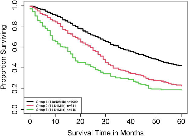
This example illustrates how to use ${\mathit{ES}}_G$ to examine differences in survival between groups. We consider three groups: Group 1, Group 2, and Group 3 defined by T1cN0M1b, T4N1M1b, and T4N1M1c, respectively. The SEER data provides us with three samples for Groups 1, 2, and 3, with sample sizes of $1009$, $311$, and $146$, respectively. Figure 1 shows the Kaplan–Meier [14] curves based on the three samples. This figure clearly indicates that the difference in survival between Group 1 and Group 2 is smaller than that between Group 1 and Group 3.

Figure 1.

Kaplan–Meier curves of T1cN0M1b, T4N1M1b, T4N1M1c in Example 1.

Calculation shows that ${\widehat{\mathit{ES}}}_G$ between Group 1 and Group 2 is $-0.207$ and ${\widehat{\mathit{ES}}}_G$ between Group 1 and Group 3 is $-0.374$. Since the absolute values of $-0.207$ are smaller than that of $-0.374$, assuming Group 2 and Group 3 have a similar censoring rate, we conclude that the survival difference between Group 1 and Group 2 is smaller than that between Group 1 and Group 3, which is consistent with the observation in Figure 1. Furthermore, Table 1 can be used to give a stronger comparison. Since the estimated censoring rates in Groups 1, 2, and 3 are $43.7\%$, $27.3\%$, and $21.2\%$, respectively, it follows from Table 1 that ${\mathit{ES}}_G$ between Group 1 and Group 2 is medium and ${\mathit{ES}}_G$ between Group 1 and Group 3 is large.

On the other hand, we could use statistical tests to examine the differences between groups. For instance, the $p$-values of the Gehan-Wilcoxon test between Group 1 and Group 2 and between Group 1 and Group 3 are, respectively, $4.8\times {10}^{-11}$ and $9.9\times {10}^{-22}$. These two $p$-values show that both the differences in survival between Group 1 and Group 2 and between Group 1 and Group 3 are significant. However, it is hard for us to use the $p$-values to imagine how much the differences are without looking at Figure 1. Furthermore, since $9.9\times {10}^{-22}$ is smaller $4.8\times {10}^{-11}$, we tend to conclude that the survival difference between Group 1 and Group 3 is larger than that between Group 1 and Group 2. But, it is hard for us to imagine the discrepancy between the two differences without looking at the survival curves.

This example demonstrates that even though $p$-values and effect sizes can be used to compare groups, $p$-values are in general less informative than effect sizes.

3.2 Example 2

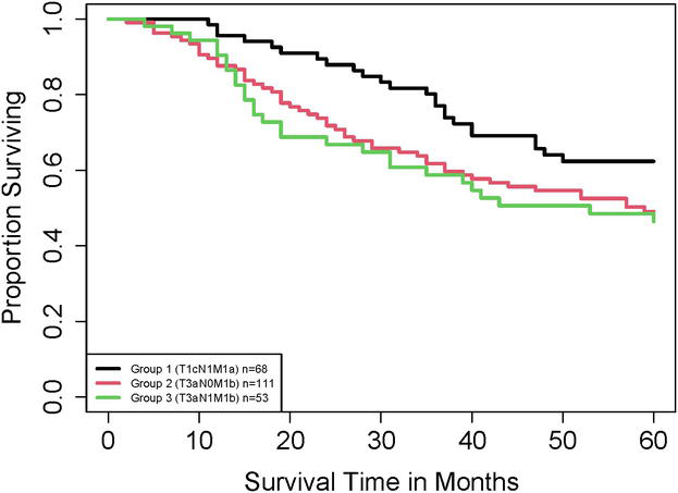
As shown in Example 1, we compute values of ${\mathit{ES}}_G$ (and censoring rates) and then use them to differentiate differences between groups. However, p-values may not be sufficient for us to do so, as illustrated in this example. Similar to Example 1, we consider three groups: Group 1, Group 2, and Group 3 defined by T1cN1M1a, T3aN0M1b, and T3aN1M1b, respectively. Note that these groups are different from those in Example 1. The SEER samples for Groups 1, 2, and 3 have sizes of $68$, $111$, and $53$, respectively. Figure 2 shows the Kaplan–Meier curves of the three samples. This figure indicates that the difference in survival between Group 1 and Group 2 is smaller than that between Group 1 and Group 3.

Figure 2.

Kaplan–Meier curves of T1cN1M1a, T3aN0M1b, T3aN1M1b in Example 2.

Calculation shows that ${\mathit{ES}}_G$ estimates between Group 1 and Group 2 and between group 1 and group 3 are $-0.168$ and $-0.198$, respectively. The estimated censoring rates in Groups 1, 2, and 3 are $58.8\%$, $48.6\%$, and $47.2\%$, respectively, so, from Table 1, ${\mathit{ES}}_G$ between Group 1 and Group 2 is medium and ${\mathit{ES}}_G$ between group 1 and group 3 is large. Thus, the difference in survival between Group 1 and Group 2 is smaller than that between Group 1 and Group 3, which is consistent with the observation in Figure 2.

If using the Gehan-Wilcoxon test to examine the differences between groups, the $p$-values of the test between Group 1 and Group 2 and between Group 1 and Group 3 are, respectively, $0.0259$ and $0.0271$. Since $0.0259$ is smaller than $0.0271$, with our common rule that a smaller $p$-value shows more significance, we would conclude that the survival difference between Group 1 and Group 2 is bigger than that between Group 1 and Group 3. Unfortunately, this conclusion contradicts our observation in Figure 2.

This example demonstrates a) a smaller $p$-value does not always mean a more significant result (See more related simulation results in [9].); and b) effect sizes can differentiate differences between groups when $p$-values fail to do so.

3.3 Example 3

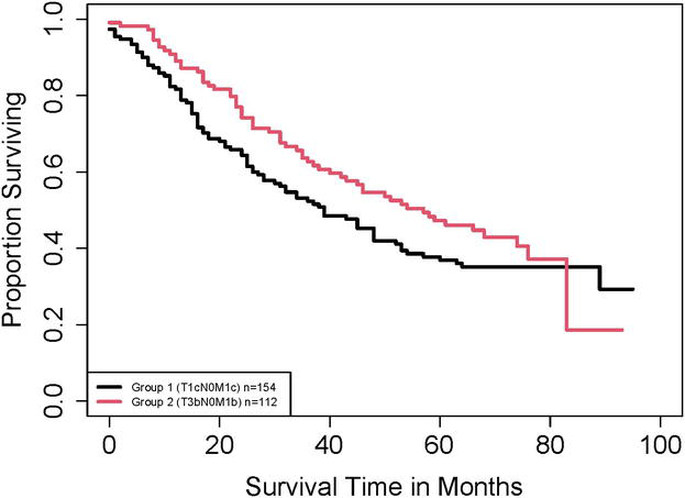
The proposed effect sizes can be applied no matter if hazards are proportional. Here we present one example with non-proportional hazards, which ${\mathit{ES}}_G$ can be applied to study the difference between two groups, while the hazard ratio approach fails to do so. We consider the following two groups: Group 1 and Group 2 defined to be T1cN0M1c and T3bN0M1b, respectively. The samples for Groups 1 and 2 have sizes of $154$ and $112$, respectively. Figure 3 shows the Kaplan–Meier curves of the two samples. This figure indicates a clear difference in survival between Group 1 and Group 2.

Figure 3.

Kaplan–Meier curves of T1cN0M1c and T3bN0M1b in Example 3.

The Grambsch–Therneau test [15] for examining the proportional hazard assumption gives a p-value of $0.012$, suggesting that the ratio of hazard rates would depend on time and thus would not be an appropriate effect size. Regardless of the violation of the proportional hazards assumption, the use of the Cox proportional hazards model would provide an estimated hazard ratio (Group 1 over Group 2) of $1.264$ with a wide confidence interval (CI) ($95\%$ CI: $0.913$ to $1.751$). These estimates are not very informative when assessing if the two groups differ in survival. Therefore, the hazard ratio approach should not be used to examine the survival difference between Group 1 and Group 2.

In comparison, the $p$-value of the Gehan-Wilcoxon test is $0.026$, which shows a significant difference in survival between Group 1 and Group 2. With effect sizes, we have ${\widehat{\mathit{ES}}}_G=0.14$ ($95\%$ CI: $0.02$ to $0.26$, a bootstrap CI [16] based on 100,000 bootstrap samples). Note that the CI does not contain $0$, so the two groups differ in survival. Furthermore, the positive effect size indicates that Group 1 has a shorter survival than Group 2. Since the censoring rates in Group 1 and Group 2 are $42.2\%$ and $44.6\%$, respectively, from Table 1, we see that there is a medium effect size between the two groups.

This example demonstrates an application of the effect size ${\mathit{ES}}_G$ to measure the difference in survival between two groups where the proportional hazards assumption does not hold. With non-proportional hazards, the traditional hazard ratio in general can not serve as an effect size.

As shown above, the effect size ${\mathit{ES}}_G$ has direct applications in practice. It is particularly useful when repeated comparisons of survival differences are required. For instance, when integrating additional variables/factors into the TNM staging system for cancer, assessing the survival difference is needed for many pairs of groups and two groups can be merged if the effect size assessing their survival difference is small. See [17, 18] for studies that applied the effect size ${\mathit{ES}}_G$ and the Ensemble Algorithm for Clustering Cancer Data [19, 20, 21, 22, 23, 24] to update and improve the staging system for thyroid and ovarian cancers.

4. Conclusion

We have reviewed the effect size ${\mathit{ES}}_G$ and its estimate for comparing the survival difference between two groups. The effect size ${\mathit{ES}}_G$ quantifies the survival difference between two groups over the time period of investigation. One can claim a small or big difference in survival according to the effect size and the censoring rates. This is different from checking the $p$-value of a statistical test, which may not provide any insight into the size of the survival difference and could cause misunderstanding. ${\mathit{ES}}_G$ can be applied no matter if hazards are proportional. This is different from the use of the hazard ratio, the traditionally used effect size. Applications of hazard ratios require the assumption of proportional hazards. With non-proportional hazards, hazard ratios can fail to detect and quantify the difference between two groups. We have also used ${\mathit{ES}}_G$ to compare different groups of patients with prostate cancer. The results have shown that ${\mathit{ES}}_G$ is a promising effect size for studying differences in survival between two groups.

There is a need for further research and refinement for our study, which currently focuses on unadjusted comparison. Our future research endeavors will delve into the exploration of incorporating methodologies that can be used to adjust important variables, such as matching, stratification, and inverse probability weighting. This future work will broaden the scope of scenarios in which ${\mathit{ES}}_G$ can be effectively utilized.

Acknowledgments

This study is based upon work supported by John P. Murtha Cancer Center Research Program under the Grant No. 64349-MCC Comprehensive Research.

Disclaimer

The contents, views, or opinions expressed in this publication or presentation are those of the authors and do not necessarily reflect the official policy or position of the Uniformed Services University of the Health Sciences, the Department of Defense (DoD), or Departments of the Army, Navy, or Air Force, or the U.S. Food and Drug Administration. Mention of trade names, commercial products, or organizations does not imply endorsement by the U.S. Government.

References

1.Amrhein V, Greenland S, McShane B. Scientists rise up against statistical significance. Nature. 2019;567:305-307
2.Wasserstein R, Schirm A, Lazar N. Moving to a world beyond “p<0.05”. American Statistician. 2019;73(Supplement 1):1-19
3.Sullivan G, Feinn R. Using effect size—Or why the P value is not enough. Journal of Graduate Medical Education. 2012;4(3):279-282
4.Cohen J. Statistical Power Analysis for the Behavioral Sciences. Revised ed. Hillsdale, NJ, US: Lawrence Erlbaum Associates, Inc.; 1977
5.Cox D. Regression models and life-tables. Journal of the Royal Statistical Society: Series B (Methodological). 1972;34(2):187-202
6.Uno H, Claggett B, Tian L, Inoue E, Gallo P, et al. Moving beyond the hazard ratio in quantifying the between-group difference in survival analysis. Journal of Clinical Oncology. 2014;32(22):2380
7.Schemper M, Wakounig S, Heinze G. The estimation of average hazard ratios by weighted Cox regression. Statistics in Medicine. 2009;28(19):2473-2489
8.Royston P, Parmar MK. The use of restricted mean survival time to estimate the treatment effect in randomized clinical trials when the proportional hazards assumption is in doubt. Statistics in Medicine. 2011;30(19):2409-2421
9.Wang H, Chen D, Pan Q, Hueman MT. Using weighted differences in hazards as effect sizes for survival data. Journal of Statistical Theory and Practice. 2022;16(1):12
10.Wang H. Development of Prognostic Systems for cancer Patients. USA: The George Washington University; 2020
11.Gehan EA. A generalized Wilcoxon test for comparing arbitrarily singly-censored samples. Biometrika. 1965;52(1-2):203-224. DOI: 10.2307/233382
12.Surveillance, Epidemiology, and End Results (SEER) Program (www.seer.cancer.gov) Research Data (2000-2020), National Cancer Institute, DCCPS, Surveillance Research Program, released April 2023, based on the November 2022 submission. Available from: https://seer.cancer.gov/
13.Edge SB, Byrd DR, Compton CC, Fritz AG, Greene FL, Trotti A. AJCC Cancer Staging Manual. 7th ed. New York: Springer-Verlag; 2010
14.Kaplan EL, Meier P. Nonparametric estimation from incomplete observations. Journal of the American Statistical Association. 1958;53:457-481
15.Grambsch PM, Therneau TM. Proportional hazards tests and diagnostics based on weighted residuals. Biometrika. 1994;81(3):515-526
16.Davison AC, Hinkley DV. Bootstrap Methods and their Application. Cambridge University Press; 1997. Available from: https://www.amazon.com/Bootstrap-Application-Statistical-Probabilistic-Mathematics/dp/0521574714
17.Yang CQ, Gardiner L, Wang H, Hueman MT, Chen D. Creating prognostic systems for well-differentiated thyroid cancer using machine learning. Frontiers in Endocrinology. 2019;10:288
18.Grimley PM, Liu Z, Darcy KM, Hueman MT, Wang H, Sheng L, et al. A prognostic system for epithelial ovarian carcinomas using machine learning. Acta obstetricia et gynecologica Scandinavica. 2021;100(8):1511-1519
19.Chen D, Xing K, Henson D, Sheng L, Schwartz AM, Cheng X. Developing prognostic systems of cancer patients by ensemble clustering. Journal of Biomedicine & Biotechnology. 2009;2009:632786. DOI: 10.1155/2009/632786. Available from: https://www.ncbi.nlm.nih.gov/pmc/articles/PMC2702512/
20.Hueman MT, Wang H, Yang CQ, Sheng L, Henson DE, Schwartz AM, et al. Creating prognostic systems for cancer patients: A demonstration using breast cancer. Cancer Medicine. 2018;7(8):3611-3621
21.Hueman M, Wang H, Henson D, Chen D. Expanding the TNM for cancers of the colon and rectum using machine learning: A demonstration. ESMO Open. 2019;4(3):e000518
22.Hueman M, Wang H, Liu Z, Henson D, Nguyen C, Park D, et al. Expanding TNM for lung cancer through machine learning. Thoracic Cancer. 2021;12(9):1423-1430
23.Yang CQ, Wang H, Liu Z, Hueman MT, Bhaskaran A, Henson DE, et al. Integrating additional factors into the TNM staging for cutaneous melanoma by machine learning. PLoS One. 2021;16(9):e0257949
24.Wang H, Liu Z, Yang J, Sheng L, Chen D. Using machine learning to expand the Ann Arbor staging system for Hodgkin and Non-Hodgkin lymphoma. BioMedInformatics. 2023;3(3):514-525
Written By
Huan Wang, Li Sheng and Dechang Chen
Submitted: 14 September 2023Reviewed: 19 September 2023Published: 11 December 2023