Cosmology with Time-Varying Curvature: A Summary

Abstract

We present a new model of cosmology based on the idea that the curvature of the universe varies with time. This model predicts a present-day exponential acceleration of the expansion of the universe without reference to a cosmological constant. We propose a new model of nucleosynthesis that accounts for the existence of cosmic structures, provides a solution to the matter/antimatter asymmetry problem, and explains the origin of the CMB. We show that this process was regulated by a vacuum imprint that came into existence during an initial Planck era inflation. One consequence is that all cosmic structures came into their final form with their present-day mass more or less simultaneously at a time of about $3\times {10}^{16}\mathrm{s}$. This explains the recent findings by the James Webb telescope of very large galaxies dating from that epoch. We show that the stability of galaxies and galaxy clusters demands that all galaxies must have developed supermassive black holes at that time. We go on to show that the phenomena attributed to dark matter are actually consequences of vacuum energy, that the conventional model for the CMB spectrum is wrong and finally, we resolve the Hubble tension problem.

1. Introduction

It has long been thought that the $\mathrm{\Lambda CDM}$ model was the final answer to the problem of the evolution of the universe and that only a few tweaks would be needed to complete our understanding of cosmology. In recent years, however, researchers have begun to realize that the standard model has serious problems that cannot be resolved by making minor adjustments. A number of papers (see e.g. [1, 2]) have recently been published that suggest that the standard model might need to be scraped in favor of new physics. In these notes, we summarize just such a model. This new model that makes a major departure from the standard model in terms of its viewpoint of the evolution of the universe while making detailed predictions that solve a large number of the outstanding problems of cosmology.

We will begin with a brief review the assumptions underlying the standard model and contrast these with those of the new model. First, the standard model assumes that the universe is homogeneous and isotropic on large scales. In the new model, we also make that assumption with, however, a major difference. Whereas the standard model asserts that the curvature of spacetime is constant, we assert that it varies with time and the consequences of that are huge. With time-varying curvature, the universe must undergo a present-day exponential acceleration of its expansion that has nothing to do with a cosmological constant. According to [1], one of the major problems of the $\mathrm{\Lambda CDM}$ model is that it cannot explain the magnitude of the cosmological constant. That of course, is not a problem in the new model because the cosmological constant simply does not exist.

Another fundamental problem with $\mathrm{\Lambda CDM}$ is that it cannot explain the “coincidence” that the present-day energy densities of the vacuum and matter are roughly the same whereas at the time of nucleosynthesis, they differed by many orders of magnitude. The new model demands that such a disparity must exist and, in fact, makes an accurate prediction of its magnitude.

The second major assumption of the standard model is that the matter distribution of the early universe was uniform. The most striking feature of the universe we observe is its fantastic degree of organization on all scales from stars up to the cosmic web. The standard model asserts that early quantum fluctuations seeded later accretions that became the structures but it is clear that this organization could not have been the result of random events so some organizing principle must have been responsible. Further, we will see that the scale of the largest structures demands that the definition of these structures came about in the absence of causality. The new model solves this problem by asserting that a blueprint that came into existence during an initial Planck era inflation later regulated nucleosynthesis in such a manner as to create all the cosmic structures we now observe.

A third major assumption of the standard model is that all cosmic structures are a consequence of accretion. We will show instead that when vacuum energy is included in Einstein’s equations, accretive structure formation initiated by small perturbations is impossible. In the new model, it was the imprint expressing itself by regulating the creation of matter that was responsible for the structures. We go on to show that after nucleosynthesis, under the influence of initially the expansion and later gravitation, the initial matter distributions became fully formed stars, galaxies, galaxy clusters, and superclusters more or less simultaneously at around $3\times {10}^{16}\mathrm{s}$ or $z\ge 6$. This is an important point because it explains the recent findings of the James Webb telescope of large fully formed galaxies with ages too great to be explained by accretion. We also show that as part of this process, all galaxies must have formed supermassive black holes because they would have otherwise undergone free-fall collapse and that radiation from galaxies interior to galaxy clusters was the agent that prevented the clusters from also undergoing free-fall collapse.

Another major problem with the standard model is that it cannot explain the matter/antimatter asymmetry of the universe which the new model does.

The chapter is a distillation of the results presented in the series of papers listed in the reference section. We ask the reader to refer to those papers for detailed discussions and references to methods and data.

One final point is that this model should be considered as a whole instead of the collection of disjoint pieces which is the case with the standard model. The present-day Hubble constant, the present-day CMB temperature, and one other parameter associated with neutron decay, fix all the parameters of the model. There are no other parameters and, unlike the situation with the standard model, only one evolution is possible.

2. Origins and the Planck era

We will begin with an observation concerning the CMB spectrum that will lead us back to the origins of everything. In spite of the claims of the standard model, superclusters are the only structures in existence large enough to be responsible for the large peaks of the CMB spectrum. In our original paper [3], we argued that superclusters were actually responsible but we have since realized [4] that the process that created the superclusters simultaneously created the CMB spectrum with peaks of the same physical dimensions. We will have more to say about this later but the point here is that superclusters in some form must have been in existence at the time of recombination. We also know that the CMB spectrum peaks were vastly too large to be explained by any causal process. Starting at the time of recombination and moving backward, since nothing much happened between the time of recombination and nucleosynthesis, it is natural to suppose that superclusters and the CMB spectrum originated during nucleosynthesis and, indeed, their material manifestation did originate at that time. Because of causality, however, the blueprint that regulated their creation must have come into existence even earlier. The only possible conclusion is that, even though causality is a cornerstone of physics that applies to most of the history of the universe, there must have been an epoch at the beginning during which it had no meaning. The final jump backward is to a Planck-era inflation.

Imagine that we are interested in measuring the duration of some event. To do so, we need a clock whose ticks are of a shorter duration than that of the event so to measure events of shorter and shorter duration, we must keep subdividing the ticks. We eventually come to a limit which we take to be the Planck time at which our ticks can no longer be subdivided. A consequence is that time becomes uncertain. The same idea holds for distance and energy as well. Since neither time nor distance had any exact meaning, it follows that causality had no meaning so during this epoch the constraints imposed by causality (and entropy) did not exist.

Such inflation by itself, however, does not explain superclusters or anything else so structure is needed. We concluded that large smooth acausal vacuum structures or imprints came into existence with relative dimensions ranging from that of stars and on up to that of superclusters and beyond. Further, we show in Section 18 that the distribution of these imprints was fractal with a dimension of about 1.1. The problem then is to account for the existence of these imprints. Given the extremely short period involved and the lack of causality, it should be clear that no complicated dynamics could have been involved. Having a fractal dimension suggests that self-similarity was in some way responsible.

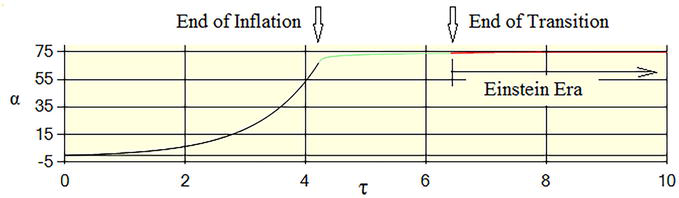
In Figure 1, we summarize the situation. The scaling is defined by $a\left(t\right)=a_P{\mathrm{e}}^{\alpha \left(t\right)}$ where $\tau =ln\left(t/t_P\right)$. The subscript “${}_P$” indicates a Planck value. The exponential expansion ended when the age of the universe became large compared to the Planck time (at about $t=6.2\times {10}^{-42}\mathrm{s}$.) Following that expansion, a transition period occurred ending at a time of about $t=6.8\times {10}^{-41}\mathrm{s}$. From that point onwards, the evolution of the universe could be described by Einstein’s equations with the understanding that Einstein’s equations have validity only for dimensions large compared to Planck dimensions. (That last statement is not an argument in support of quantum gravity which we contend does not exist. Instead, at the Planck limit, a point in spacetime does not have any precise meaning so any normal concept of dynamics cannot exist.)

Figure 1.

Initial evolution of the universe.

As we will see in the next section, in the new solution of Einstein’s equations, the scaling of the universe is entirely a consequence of the vacuum and since the model contains no free parameters, we can work backward from the present day to fix the value of the scaling at the end of the transition.

We recognize that there is no direct observational evidence that inflation existed and, in fact, there never can be for the simple reason that there was nothing to observe before nucleosynthesis. The indirect evidence for inflation, on the other hand, is overwhelming given the assumption that the Big Bang expansion began from a Planck-sized beginning. The fact that the new model solution must join onto the scaling at the end of the transition not only constrains the magnitude of the inflation, it also forces the conclusion that there was an inflation. In fact, without the inflation, the present-day size of the universe would be a small fraction of a meter.

Any discussion of a Planck era eventually brings up the point the Planck dimensions are simply dimensional constructs based on the values of certain physical constants and it would be a fantastic coincidence if the actual Planck dimensions were the same as the constructs. However, a possible resolution to this dilemma is achieved if we turn the Planck dimension formulas around giving us the origin of the physical constants, e.g. $\mathrm{c}={\mathrm{l}}_{\mathrm{P}}/{\mathrm{t}}_{\mathrm{P}}$ and so on.

3. A new model of the Einstein era

By the end of the transition period, the uncertainties would have become negligible and normal causality would have come into play. The development of the new model, [3], begins with the idea that the universe consists of a sequence of hyperspheres each of which is homogeneous and isotropic (the real universe as opposed to our preception of the universe.) The standard model goes on to assume that the curvature of each of these hyperspheres has a single, constant value but there is no physical principle that says that must be the case. We instead assert that the curvature varies with time.

We now need to connect these hyperspheres with Einstein’s equations. Given the assumptions of homogenity and istropy, the hyperspheres can have no preferred origin and all their properties are dependent only on time. Our perception of the universe, on the other hand, is concerned with signals, causality, and so on and these are dependent on both time and distance as described by Einstein’s equations. The question, then, is how do we reconcile the equations that describe our perception with a sequence of hyperspheres that have no notion of an origin or distance? The answer is that Einstein’s equations describe the universe from the viewpoint of each observer. But a hypersphere is simply the collection of all possible observer origins so Einstein’s equations become the equations that describe the hypersphere when evaluated at any observer’s origin. Said another way, separations on a hypersphere are space-like and since Einstein’s equations describe time-like events, the only possible point of contact is with a signal of zero spatial extent. Einstein’s equations have nothing to say about points with spacelike separations which is the reason that Einstein’s equations can accommodate multiple viewpoints of cosmology.

In the standard model, the additional assumption is made that not only are the hyperspheres homogeneous and isotropic but that the universe must appear homogeneous and isotropic. With time-varying curvature, on the other hand, the metric must contain an off-diagonal term connecting time with distance with the result that the universe will not appear homogeneous and isotropic to an observer. As we will show, however, the difference only becomes apparent at very large redshifts.

Putting these ideas together, the metric becomes,

$$\begin{array}{ll}{\mathit{ds}}^2& =\left(-1+\frac{r^{2}h{\left(\mathit{ct},r\right)}^2}{a{\left(\mathit{ct}\right)}^2}\left(1-k\left(\mathit{ct}\right)r^2\right)\right){\left(\mathit{cdt}\right)}^2\\ & +2h\left(\mathit{ct},r\right)\left(\mathit{cdt}\right)\mathit{rdr}+a^2\left(\mathit{ct}\right)\left(\frac{{\mathit{dr}}^2}{\left(1-k\left(\mathit{ct}\right)r^2\right)}+r^{2}d{\mathrm{\Omega }}^2\right).\end{array}$$E1

The second part of the new model concerns the vacuum energy density. Instead of the standard model concept of a vacuum described by ${\mathbf{T}}^{\mathit{\mu \nu }}=0$, the new model vacuum acts as its own source so we have

$${\mathbf{T}}^{\mathit{\mu \nu }}=\left({\rho }_{\mathit{vac}}{c}^2\left(\mathit{ct},r\right)+p_{\mathit{vac}}\left(\mathit{ct},r\right)\right){\delta }_0^{\mu }{\delta }_0^{\nu }+p_{\mathit{vac}}\left(\mathit{ct},r\right)g^{\mathit{\mu \nu }}.$$E2

After working out Einstein’s equations and taking the limit as $r\to 0$, the resulting equations can be solved in closed form. The scaling is given by,

$$a\left(\mathit{ct}\right)=a_{\ast }{\left(\frac{\mathit{ct}}{{\mathit{ct}}_0}\right)}^{{\gamma }_{\ast }}{\mathrm{e}}^{\frac{\mathit{ct}}{{\mathit{ct}}_0}{c}_1},$$E3

where

$$a_{\ast }=a_0{\mathrm{e}}^{-c_1}.$$E4

(Ref. [3] for the omitted definitions). We see that the scaling is power-law for $\mathit{ct}/{\mathit{ct}}_0\ll 1$ and exponential for $\mathit{ct}/{\mathit{ct}}_0\ge 1$. The curvature is given by

$$k\left(\mathit{ct}\right)={\overline{k}}_0{\left(\frac{a\left(\mathit{ct}\right)}{\mathit{ct}}\right)}^2$$E5

which is related to the vacuum energy density and pressure by

$$k\left(\mathit{ct}\right)=\frac{1}{2}{\gamma }_{h}a{\left(\mathit{ct}\right)}^2\kappa \left({\rho }_{\mathit{vac}}{c}^2\left(\mathit{ct},0\right)+p_{\mathit{vac}}\left(\mathit{ct},0\right)\right).$$E6

The sum is thus a fixed function of time,

$${\rho }_{\mathit{vac}}{c}^2\left(\mathit{ct},0\right)+p_{\mathit{vac}}\left(\mathit{ct},0\right)=\frac{2{\overline{k}}_0}{\kappa {\left({\mathit{ct}}_0\right)}^2{\gamma }_h}\frac{{\left({\mathit{ct}}_0\right)}^2}{{\left(\mathit{ct}\right)}^2}.$$E7

Note that there is no direct relationship between the scaling and the energy density or pressure. The present-day acceleration of the scaling is, in fact, a kinematic constraint that follows directly from the time variation of the curvature and the presence of the vacuum energy in the energy-momentum tensor. It has nothing to do with a cosmological constant or so-called dark energy. This situation is completely different from that of the standard model based on the FRW solution of Einstein’s equations. The latter does not actually predict anything based solely on being a solution to the equations. By making choices about various parameters, it is possible to predict any sort of evolution one cares to see. In the new model that is not the case. There is one solution and only one evolution is possible.

Both the energy density and the pressure contain a constant term that one might think to associate with a cosmological constant. If we must assign a meaning to these constants, they are the values of the vacuum energy and pressure at infinite time. These, however, have no physical consequences and they can be removed by simply adding a constant term to the energy-momentum tensor. Physical quantities such as the curvature are functions of the sum rather than either energy or pressure individually and in the sum, the constant terms cancel.

Aside from the present-day size and age of the universe, we need the value of the scaling at two different times to fix the parameters of the model. For one, we use a present-day value of the Hubble constant. There is some uncertainty about its value but, as we will show later, a consensus of $H_0=73{\mathrm{kms}}^{-1}{\mathrm{Mpc}}^{-1}$ is emerging from the various methods used to determine its value. For the other parameter, we use the energy density of the CMB at the time of nucleosynthesis. From this, we determine that ${\gamma }_{\ast }$ can be at most only slightly greater than ½. For the model development, we needed to assign a single value which we chose to be exactly ½. The relationship between the Hubble constant and the model parameters is $c_1=t_0{H}_0-{\gamma }_{\ast }$ from which we determine that $c_1$ always has a value close to ½. For $H_0=73$ we have $c_1=0.525$.

There appears to be one remaining parameter, namely $k_0$. During and shortly after the inflation, the curvature was maximal which motivates an additional principle that states that the curvature must always be as large as possible or equivalently, that the vacuum energy density must always be as large as possible. From the solution, it then follows that $k_0=1.41$.

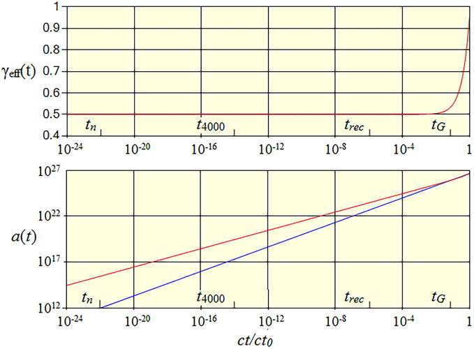
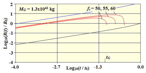
Everything is now fixed and unambiguous predictions can be made. We define an effective scaling parameter by $a\left(t\right)=a_0{e}^{{\gamma }_{\mathit{eff}}\left(t\right)}$ which we show in Figure 2. We also show the scaling as a function of time. The exponential acceleration of the scaling is clearly visible.

Figure 2.

The time-varying curvature predictions are shown in red. For comparison, the curve for $2/3^{\mathit{rds}}$ scaling is shown in blue. The indicated times are $t_n$ = the time of neutron formation to be explained below, $t_{4000}$ = the end of nucleosynthesis, $t_{\mathit{rec}}$ = the time of recombination, and $t_G$ = the time of galaxy formation.

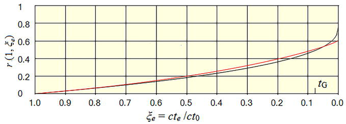
In Figure 3, we show the coordinate distance of sources whose signals are received at the present plotted as a function of the lookback time. Both time-varying and constant curvature cases are shown. The two curves are similar for small values of look-back time but they differ considerably for large redshifts which illustrates the point we made earlier about the universe not appearing homogeneous and isotropic. In particular, with time-varying curvature, there is a fundamental limitation on our ability to detect distance sources. No matter how far back in time we look, we cannot see sources with coordinate distances greater than about $r=0.6$. This is in direct contrast to the standard model where no such limitation exists.

Figure 3.

$r\left(1,{\xi }_e\right)$ vs. ${\xi }_e$. The red curve is the time-varying curvature result. For comparison, we also show in black the result computed assuming a constant value of $k=1$.

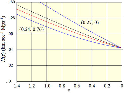
The redshift dependence of the Hubble parameter, $H\left(t\right)\equiv \dot{a}\left(t\right)/a\left(t\right)$, is shown in Figure 4.

Figure 4.

Hubble parameter vs. redshift. Time-varying curvature in red, constant curvature in black. The FRW results for two values of the densities are shown in blue. The latter were normalized to the value of the new model curve at $z=0$.

Finally, the model makes a prediction of the luminosity distances of various sources that agree with observation but we will postpone that discussion until we reach the section concerned with the Hubble tension problem.

Up to this point, we have only considered the vacuum but eventually, particles permeated space so we need to consider their interaction with the vacuum energy density. On the LHS of Einstein’s equations, the connection coefficients depend only on the metric components and these have no dependence on either the vacuum energy density or pressure. On the RHS, since the particles can be assumed to be at rest, their density is simply added to the vacuum energy density. Ordinarily, after including a new term, we would need to re-solve the equations but in this case, the equations have not changed since the particle density just becomes part of the vacuum energy sum so the original solution still holds. This means that any small variation in the particle density will be immediately canceled by the corresponding variation in the vacuum needed to keep the sum unchanged. Since the gravitational field does not change, nearby matter will not detect any difference in the field so no accretion occurs. When the vacuum energy is included, Einstein’s equations show that accretion initiated by small particle density fluctuations is impossible.

We can now address the “coincidence” problem mentioned in the introduction. From (Eq. (7)), we find that the present-day vacuum energy density sum is

$$\rho c^2\left({\mathit{ct}}_0,0\right)+p\left({\mathit{ct}}_0,0\right)=2.1\times {10}^{-10}\mathrm{j}{\mathrm{m}}^{-3}$$E8

which differs from the value of the so-called dark energy density ($6.3\times {10}^{-10}\mathrm{j}{\mathrm{m}}^{-3}$) by no more than a factor of three. Note, however, that even though the magnitudes are similar, these are in no way equivalent. The notion of dark energy driving the acceleration of the scaling just does not exist in the new model. If we assume that the average present-day particle density is about $1{\mathrm{m}}^{-3}$, we find a matter energy density equal to $E_{\text{part}}\left(t_0\right)=1.5\times {10}^{-10}\mathrm{j}{\mathrm{m}}^{-3}$ and comparing with the vacuum value, we find that they are essentially the same. Now, using the scaling of (e.g. (3)), we determine that the particle energy density at $t=1\mathrm{s}$ was $E_{\text{part}}\left(1\mathrm{s}\right)=2.1\times {10}^{17}\mathrm{j}{\mathrm{m}}^{-3}$ and from (Eq. (7)), that the vacuum energy density was $E_{\mathrm{vac}}\left(1\mathrm{s}\right)=4.0\times {10}^{25}\mathrm{j}{\mathrm{m}}^{-3}$. The latter is larger than the particle energy density by eight orders of magnitude. Thus, what is a great problem for the standard model is a non-issue in the new model. The vast change in the energy density ratio over time is an unavoidable consequence of time-varying curvature.

4. Nucleosynthesis

The next step is to account for the creation of ordinary matter. We begin by separating what is known from what is conjecture. Observations of galaxies allow the relative abundances of the light elements to be measured. Working backward in time, the abundances at the end of nucleosynthesis can then be estimated because the processes that occurred during the intervening period are known. Similarly, the nucleosynthesis reactions are also known so one can work backward again to discover what densities of protons and neutrons were necessary to account for the abundances of the light elements. We can also establish that the process began at a time of about ${10}^{-5}\mathrm{s}$. That, however, is as far as one can go. Whatever happened before that time is beyond the reach of even extrapolations of observations. This means, for example, that there is no evidence to support the standard model’s field theory beginning. There is also no evidence to support the standard model’s assumption that the initial baryon density was uniform throughout the universe.

Here, we will propose a much simpler model, [3, 4] that leads to the same nucleosynthesis starting point but which also accounts for the matter/antimatter asymmetry of the universe, the existence of the CMB, and the high density of neutrinos needed to establish the pre- nucleosynthesis proton/neutron abundance ratio. We start with the idea that there was no existence other than the vacuum prior to the time of nucleosynthesis and that at that time, a very small percentage of the vacuum energy was converted into neutron/antineutron pairs with a very small bias of 2–4 extra neutrons for every ${10}^8$ pairs. Using the formula for the energy density of the vacuum given earlier and assuming that the pair production occurred at the point in time when the vacuum energy density equaled the equivalent energy density of a neutron, we determine that the event occurred at a time of $t_n\approx 4\times {10}^{-5}\mathrm{s}$.

Initially, we have neutrons and antineutrons but we also need protons. Our original idea was that weak interactions were responsible for the existence of the protons but that turned out to be wrong. The weak interactions did play a critical role but they were not responsible for the original population of protons. Instead, the protons and antiprotons were a consequence of baryonic charge exchange reactions, [4].

Starting with the neutrons and antineutrons, particle/antiparticle annihilation and charge exchange reactions proceeded at a very high rate creating, in addition to protons and antiprotons, a very high density of mesons, neutrinos and electrons along with the radiation that became the CMB. Ultimately, the small excess of initial neutrons resulted in the matter/antimatter asymmetry of the universe. This entire process was very fast and was completed ${10}^{-12}\mathrm{s}$ after it began. At the end of this process, there were equal numbers of protons and neutrons but soon afterward, weak interactions became important and it was these that adjusted the proton/neutron ratio to the value it had when nucleosynthesis proper began.

The key point about this process is that it was not random. Instead, it was regulated by the Planck era imprint that we spoke of earlier. This imprint caused an increase relative to the average in the number of neutrons and antineutrons in the regions that became the cosmic structures and a decrease in the regions that became the voids.

For this to work, there must have been a universal violation of the baryon conservation law because the same excess had to have occurred everywhere and so cannot be the result of some random process. In fact, to account for the matter/antimatter asymmetry, some such violation must be introduced no matter what creation model is assumed. Indications of such a violation in connection with neutrons have been known for a long time. The evidence, known as the neutron enigma, comes from experiments conducted to determine the half-life of the neutron. The problem is that different values result depending on the design of the experiment, (see reference in [3]). Experiments that detect the protons that result from the neutron decay give one value and experiments that count the total number of neutrons remaining in a container as a function of time gives another value. The difference is evidence that some of the neutrons simply disappear without leaving behind any daughter particles.

Referring now to the problems listed in [1], there are several that can now be settled. There are several supposed anomalies with the CMB spectrum that are again artifacts of the $\mathrm{\Lambda CDM}$ model. Problems such as the CMB cold spot, cosmic hemispherical power asymmetry, the lack of large-angle CMB temperature correlations, the cosmic dipole problem, and the galaxy cluster count problem among others do not exist in a universe in which the creation of matter (and radiation) was regulated by a fractal vacuum imprint. The universe began with structure instead of with a uniform matter distribution.

We will discuss this initial stage of nucleosynthesis more fully in a later section but to appreciate the details of this process, we first need to examine the subsequent development of cosmic structures.

5. The origin of cosmic structures

Skipping over the details of nucleosynthesis proper, we will now consider the problem of how the proton gas that resulted from nucleosynthesis became the structures we now observe. The filament structure that defines superclusters was fixed by the nucleosynthesis process discussed above and because the filaments are vastly too large to undergo gravitational evolution, they are much the same today as they were initially. The components that make up the filaments such as galaxy clusters, on the other hand, did evolve.

To study the initial evolution of all smaller cosmic structures, we consider the motion of a particle lying at the outer edge of a volume containing the mass that eventually became the structure in question, [5]. The only accelerations acting on the particle were gravitation and the acceleration due to the expansion of the universe so the equation of motion of the particle becomes

$$\begin{array}{ll}\ddot{R}\left(t\right)& =-\frac{{\mathit{GM}}_{\mathit{eff}}\left(t\right)}{R{\left(t\right)}^2}+R_0{f}_s\frac{\ddot{a}\left(t\right)}{a_0}\\ & =-\frac{{\mathit{GM}}_{\mathit{eff}}\left(t\right)}{R{\left(t\right)}^2}+R_0{f}_s\left(-{\gamma }_{\ast }+{\left({\gamma }_{\ast }+c_1\frac{t}{t_0}\right)}^2\right)\frac{a\left(t\right)}{a_0}\frac{1}{t^2}.\end{array}$$E9

The coordinate $R\left(t\right)$ is the distance from the particle to the center of the structure and

$$M_{\mathit{eff}}\left(t\right)=M_{\mathit{\text{Struct}}}\left(1-{\left(\frac{R\left(t\right)}{R_{\mathit{Sur},s}\left(t\right)}\right)}^3\right)$$E10

is the effective mass of the structure adjusted for the presence of the background particle density.

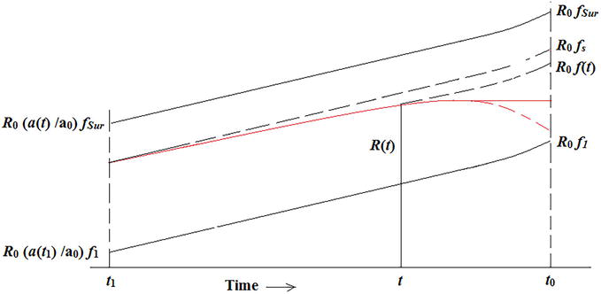
The coordinates are illustrated in Figure 5. $R_0$ is the present-day size of the structure. The parameter f is a multiplier used to define the size of any feature of interest in present-day terms. The size of the same feature at any earlier time is given by $R\left(t\right)=R_0\left(a\left(t\right)/a_0\right)f$. The black lines indicate the change in the distance due to the expansion alone. The lower black line indicates the size that would have evolved into the present-day size in the absence of gravitational acceleration (the value at $t=t_0$ is its present-day size.) The red line illustrates a possible trajectory for a particle when gravitation is included.

Figure 5.

Coordinate system for structure evolution.

If we consider a particle located at the radius of the volume needed to form any structure from the background density, nothing would happen because the density would be the same everywhere. The corresponding multiplier is $f_{\mathit{sur}}$. To get things going, we need to fix the starting radius of the volume containing the mass of the structure at a value less than the value corresponding to the background. The multiplier in this case is $f_s<f_{\mathit{sur}}$.

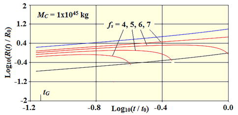
We will first consider the evolution of a galaxy cluster. In all cases, we imagine that the particles were created at rest so their initial recession velocity was fixed by the expansion. According to the accretion model of structure formation, structures could not come into existence until there was something to accrete which we take to mean that the starting time would be the generally accepted time of galaxy formation. In Figure 6, we show the model results for several values of initial over-density. The blue line is the solution for $f_s=f_{\mathit{sur}}$ and since in that case there was no gravitational acceleration, the size would follow the expansion of the universe. Considering the red lines, it is apparent that a value of $f_s<7$ is necessary for the cluster to have any chance of forming, and a value closer to 4 would be necessary to account for the present-day size. The point at which the structure ceases to expand we call the zero-velocity point (ZVP). The critical point is that the cluster must have already been a well-defined structure long before the time conventionally associated with galaxy formation.

Figure 6.

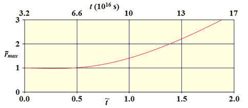
Solution for four values of the starting position with $t_s=t_G=3.2\times {10}^{16}\mathrm{s}$ and a cluster mass of $M_C={10}^{45}\mathrm{kg}$.

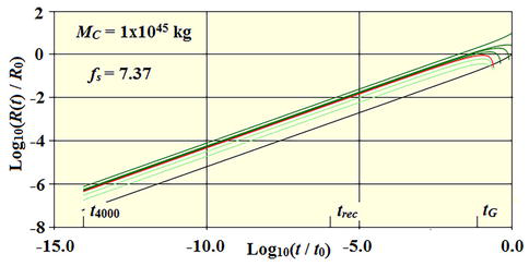
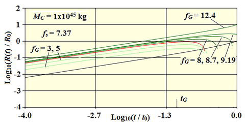
Since we have argued earlier that all structures came into existence at the time of nucleosynthesis with more or less their final mass, we recalculate the evolution beginning at the time that nucleosynthesis proper ended or about $t_s=4000\mathrm{s}$. The procedure was to run simulations with decreasing values of the initial radius but enclosing the same total mass until we obtained a structure with its present-day size. The results are shown in Figures 7 and 8. The red line shows the evolution of the cluster and we see that it reaches its ZVP at $t=t_G$ and with its present-day size. The other curves show the paths of a few internal and external galaxies. The galaxy with $f_s=12.4$ is an example of an external galaxy that was too far from the cluster to be captured.

Figure 7.

Solution with $t_{4000}=4000\mathrm{s}$ and $f_s=7.37$.

Figure 8.

Detail view of Figure 7.

The value $f_s=7.37$ corresponds to an initial compaction ratio of 1.35 or an initial density of $2.5{\mathrm{m}}^{-3}$ in present-day terms. What is apparent is that the motion of the surface was completely dominated by the expansion up until a time fairly close to $t=t_G$. Until then, the particles were moving away from each other far too rapidly for gravitation to have any effect on their evolution. The recession rate, $\dot{R}\left(t\right)=R_0\left(\dot{a}\left(t\right)/a_0\right)f$, for example, does not drop below the speed of light until a time of about ${10}^{10}\mathrm{s}$. Keep in mind that during this phase, the particles are not actually moving. Eventually, however, gravitation does begin to slow the expansion, and finally, at the time usually associated with galaxy formation, the expansion stops at the ZVP. From that point, the equations indicate that the cluster would have undergone free-fall collapse which it would have done in the absence of processes that stabilized the cluster. An interesting point about clusters is that the evolution shown for the Virgo cluster seems to apply generally to all clusters. They reach their ZVPs at a time of about $t=t_G$ with their final present-day sizes over a considerable range of masses.

6. Galaxy evolution

We will now apply the same model to galaxies, [5]. The procedure is the same as for clusters. Taking the Milky Way as our example, the outer surface parameter is $f_{\mathit{sur}}=140$. The results for three values of $f_s$ are shown in Figure 9.

Figure 9.

Galaxy evolution for three values of $f_s$ and a mass of $M_G=1.3\times {10}^{41}\mathrm{kg}$.

A value of $f_s=55$ results in a ZVP close to $t=t_G$. This corresponds to an initial proton density of about $17{\mathrm{m}}^{-3}$ in present-day terms and an initial size about 55 times its present-day size again in present-day terms. The really interesting prediction of the model, however, is that galaxies reached their ZVPs with sizes many times larger than their present-day sizes. For the Milky Way, the ratio was 5.2. This result turns out to be of critical importance. It is responsible for the existence of the observed large HI rings, [6], and as we will show below, for the existence of supermassive black holes which, in turn, were responsible for the radiation that stabilized those same galaxies and also galaxy clusters, [7].

At this point, we emphasize that in this new model of structure formation, all structures came into existence at roughly the same time with essentially all their present-day mass. Clusters had most of their complement of galaxies, and galaxies had a good supply of stars. This result is completely at odds with what has been expected based on the accretion model of galaxy formation. In the latter model, the earliest galaxies would have be fragmentary rather than fully formed. The early results from the James Webb telescope clearly support the new model viewpoint over that of the accretion model.

7. Stellar evolution

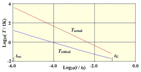
We will next move on to the stars, [5]. Although stars are extremely dense compared to everything else, that density is a consequence of their collapse. At the time of nucleosynthesis, their imprint density was only slightly larger than that of their host galaxies. For our model, we assume an initial nominal dimension of $1\mathrm{ly}$ in present-day terms. It turns out that with stars, gravitation became effective much earlier in their evolution than was the case for the larger structures. Depending on the initial value of $f_s$, stars could reach their ZVP at times even earlier than $t=t_{\mathit{rec}}$ which would imply that we could have had stars long before the formation of the galaxies or even recombination. The fact that they did not undergo early collapse is a consequence of the temperature of the gas.

According to Jean’s model of star formation, for a star to form, the sum of the potential and kinetic energies must be less than zero which results in a critical temperature of

$$T_c=\frac{0.683}{R\left(\mathit{ly}\right)}\mathrm{K}$$E11

where R is the radius of the cloud at the ZVP. Before $t_{\mathit{rec}}$, the gas was in thermal equilibrium with the CMB radiation. At $t_{\mathit{rec}}$, the gas had a temperature of about $3000\mathrm{K}$, and thereafter, the temperature of the gas decreased proportionally to $a{\left(t\right)}^{-2}$. In Figure 10, we compare the actual temperature with the critical temperature.

Figure 10.

Comparison of the actual and critical temperatures.

We find that the gas temperature did not reach the critical value until about $t=t_G$ when it had a value very close to 1 K. The result was that stars condensed into their final form at the same time as the galaxies but for a different reason.

8. Galaxy and Galaxty cluster stability

We have now established that, aside from superclusters, all structures reached their ZVPs at approximately the same time and with essentially all their present-day mass. The problem is that, without some process to prevent it, both galaxies and galaxy clusters would have undergone the gravitational free-fall collapse indicated in the figures. (The stars did undergo collapse so we are not concerned about them.). The reason that galaxies and clusters did not collapse was that their constituent gas was rapidly heated very soon after they reached their ZVPs, [7].

To model the dynamics, we used a modified form of the usual hydrodynamic equations. We assumed spherical symmetry and adopted the Lagrangian viewpoint. The final equations in terms of dimensionless coordinates are as follows;

$$\frac{\partial \overline{r}}{\partial \overline{t}}=\overline{v}$$E12

$$\frac{\partial \overline{v}}{\partial \overline{t}}=-\frac{\overline{m}}{{\overline{r}}^2}-4\pi \frac{{\tilde{\rho }}^{5/3}}{{\overline{r}}^{4/3}}\left(\frac{\partial \overline{\psi }}{\partial \overline{m}}+\frac{5}{3}\frac{\overline{\psi }}{\tilde{\rho }}\frac{\partial \tilde{\rho }}{\partial \overline{m}}\right)+\frac{10}{3}\frac{{\tilde{\rho }}^{2/3}\overline{\psi }}{{\overline{r}}^{7/3}}+\frac{\overline{r}}{{\overline{t}}^2}\left(-{\gamma }_{\ast }+{\left({\gamma }_{\ast }+c_1\frac{\overline{t}}{{\overline{t}}_0}\right)}^2\right)$$E13

$$\frac{\partial \tilde{\rho }}{\partial \overline{t}}=-4\pi {\tilde{\rho }}^2\frac{\partial \overline{v}}{\partial \overline{m}}$$E14

$$\frac{\partial \overline{\psi }}{\partial \overline{t}}=\frac{2}{3}{\left(\frac{{\overline{r}}^2}{\tilde{\rho }}\right)}^{2/3}\overline{q}.$$E15

We have defined a dimensionless time, $\overline{t}$, by

$$t=t_s\left(0.469+\overline{t}\right)$$E16

where $t_s=\sqrt{{R_c}^3/{\mathit{GM}}_C}=6.8x{10}^{16}\mathrm{s}$ so $\overline{t}$ ranges from 0 to 5.91 as t ranges from $t_G$ to $t_0$. We have eliminated the pressure in favor of the entropy function,

$$\overline{\psi }\left(\overline{t},\overline{m}\right)=\frac{p\left(\overline{t},\overline{m}\right)}{\rho {\left(\overline{t},\overline{m}\right)}^{5/3}}$$E17

and have defined an adjusted density by

$$\tilde{\rho }\left(\overline{t},\overline{m}\right)\equiv \overline{\rho }\left(\overline{t},\overline{m}\right){\overline{r}}^2.$$E18

The independent spatial coordinate, $\overline{m}$, is related to the radial coordinate by

$$\overline{m}=4\pi {\int }_0^{\overline{r}}d{\overline{r}}^{\text{'}}\tilde{\rho }\left(\overline{t},{\overline{r}}^{\text{'}}\right).$$E19

We note that these equations do not contain any dimensionless structure-dependent parameters so the solutions apply to both galaxies and clusters. Initially, the gas had a temperature of at most a few K, and because we are starting at the ZVP, $\overline{v}\left(\overline{t},\overline{m}\right)=0$. We also know their initial size and mass.

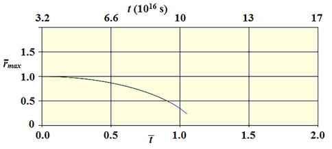
We will first consider the evolution of clusters. To establish the time scale of our problem, in Figure 11 we show the evolution of a cluster in the absence of any heating and find that the stabilization of the clusters must occur very soon after the ZVP.

Figure 11.

Cluster free-fall collapse.

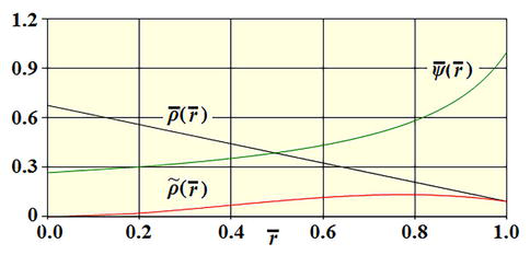
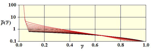
We have two problems to solve. The first is to determine what combinations of the initial density and radiation result in a cluster that neither collapses nor evaporates. The second problem is to identify the source of the radiation. We soon discovered that with a uniform initial density profile, clusters would have collapsed no matter what temperature profile is assumed. The same is also true if the profile is too sharply peaked at the origin. We tried several initial density profiles and determined that the profile must have a moderate negative slope. An example is the curve labeled $\overline{\rho }\left(\overline{r}\right)$ in Figure 12.

Figure 12.

Linear density profile with negative slope.

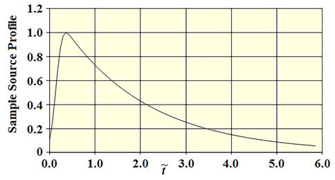
We next consider the heating. We very quickly determined that compressive heating develops far too slowly to prevent the collapse which means that a source of radiation must have been responsible. We thus needed to assume a radiation source profile and our first try was the broad profile shown in Figure 13. The sample profile has a maximum value of unity which is then scaled by a multiplier in the simulation code. With a multiplier of five, the resulting size of the cluster is shown in Figure 14. What we find is that while a significant amount of radiation is necessary to prevent the collapse, it must also be short-lived because otherwise, the cluster would have evaporated.

Figure 13.

Broad radiation profile.

Figure 14.

Solution with the density and radiation profiles of Figures 12 and 13.

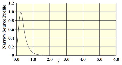
For our next try, we assumed the narrow profile shown in Figure 15 and obtained the evolution shown in Figure 16. (Narrow is a relative term, the width of the peak still amounts to $\approx {10}^9\mathrm{yr}$.) This result shows that we are on the right track. We have found a solution that neither collapses nor exhibits undue expansion. The necessary conditions are that the density profile must have a modest negative slope and that the radiation profile must rise sharply after the ZVP and then, just as quickly it must cease or nearly cease.

Figure 15.

Narrow radiation profile.

Figure 16.

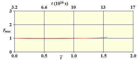
Solution with narrow radiation profile and a multiplier of 6.

The actual peak radiation intensity is given by $q_{\mathit{\text{peak}}}=f_{m}1.4x{10}^{-5}\mathrm{j}{\mathrm{kg}}^{-1}{\mathrm{s}}^{-1}$ where $f_m$ is on the order of 5 or 6. Multiplying by the mass of the cluster, the total absorbed radiation works out to be on the order of $f{10}^{40}\text{watts}$ or $f2.5\left({\mathrm{M}}_{\odot }{\mathrm{c}}^2\right){\mathrm{yr}}^{-1}$.

The final problem is to identify the source of this radiation. We need a huge power output and even more importantly, a significant lifespan and active galactic cores, or, in other words, quasars are the only real possibility. Power outputs from large quasars are on the order of ${10}^{40}\text{watts}$ which is in the range needed. A few large quasars, however, would not solve our problem. First, the released radiation would be too concentrated in some areas and insufficient in others, and second, it would have lasted too long. Instead, we need a large number of short-lived mini-quasars which would have run out of fuel in a relatively short time and become normal galaxies.

To have quasars, however, we must have supermassive black holes. We discovered earlier that galaxies would have undergone gravitational free-fall collapse soon after reaching their ZVP unless something prevented that from happening. The galaxies reached their ZVP with sizes several times larger than their present-day size and soon after did begin to collapse. Initially, the gas making up the galaxy was cold and, as was the case of the clusters, compressive heating would not have stopped the collapse. We now assert that during this contraction, all galaxies formed supermassive black holes together with accretion disks. In Figure 17, we show a calculated sequence of density profiles showing the initial phase of the collapse. We find that the density increases extremely rapidly at the origin creating the conditions necessary for the formation of a black hole and that it does so long before there is any significant reduction in the radius of the galaxy.

Figure 17.

Density profiles during the initial phase of galaxy collapse.

As the collapse continued, an accretion disk must have formed and the resulting radiation heated the galactic gas thereby stopping the collapse. The key point is that all galaxies must have formed a supermassive black hole complete with an accretion disk because they would have otherwise collapsed.

Much of that radiation would have escaped the galaxy and in the cases in which the galaxies were located inside a cluster, they would have heated the cluster gas. The Virgo cluster contains a large number of galaxies, most of which are dwarf ellipticals. References listed in [7] found that first, quasar host galaxies are all ETGs with the bulk being ellipticals and second, that dwarf ellipticals do have active nuclei. The Virgo cluster does not contain a quasar at present but it is a characteristic of active nuclei that they radiate huge amounts of energy until their supply of accretion material runs out after which they become normal galaxies. The conclusion is that clusters were heated from within by a large number of mini-quasars that collectively used up their accretion supplies within the time scale indicated in Figure 15.

9. Nucleosynthesis again

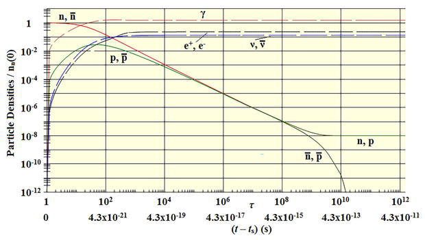
We will now return to the nucleosynthesis pair production process that we introduced earlier. To study the evolution, we created a simulation model that included neutrons, protons, electrons, neutrinos, photons, and their antiparticles. We then solved the coupled reaction rate equations to determine the evolution, [4].

As we discussed earlier, at a time of about $t_n=4\times {10}^{-5}\mathrm{s}$ a very small percentage of the vacuum energy was converted into neutron and antineutron pairs with a neutron excess of about two extra neutrons for every ${10}^8$ pairs. The list of reactions is long but the principal ones were the baryon annihilation and charge exchange reactions listed below.

$$\mathrm{n}+\overline{\mathrm{n}}\to \gamma +\text{leptons}$$E20

$$\mathrm{p}+\overline{\mathrm{p}}\to \gamma +\text{leptons}$$E21

$$\mathrm{n}+\overline{\mathrm{p}}\to \gamma +\text{leptons}$$E22

$$\overline{\mathrm{n}}+\mathrm{p}\to \gamma +\text{leptons}$$E23

$$\overline{\mathrm{p}}+\mathrm{p}\rightleftarrows \mathrm{n}+\overline{\mathrm{n}}.$$E24

(We have indicated the final states of the annihilation reactions but these actually pass through an intermediate meson state that eventually decays into the photons and leptons.) In Figure 18, we show the results for an initial density of $n_{\mathrm{n}}\left(0\right)={10}^{41}{\mathrm{m}}^{-3}$ and a neutron excess ratio of $2\times {10}^{-8}$. The whole process was completed in about ${10}^{-12}\mathrm{s}$.

Figure 18.

Initial stage of nucleosynthesis.

The simulation was primarily concerned with the baryon annihilations and the baryon curves are correct. The details of the product particle distributions, on the other hand, were of only secondary interest at the time and because we needed to keep the simulation manageable, we did not take proper account of the meson state branching ratios or the meson lifetimes which is the reason that the leptons and photon curves are shown dashed.

The annihilation decay products are primarily pions. Neutral pions decay into two photons with a relatively short mean lifetime so labeling the curve as photons is a fair representation of the actual situation. Charged pions, on the other hand, decay into muons which subsequently decay into either electrons or positrons plus neutrinos with a combined mean lifetime much larger than the time scale of the figure. That being the case, the curves labeled ${\mathrm{e}}^{+},{\mathrm{e}}^{-}$ and $\nu ,\overline{\nu }$ could more accurately be labeled ${\pi }^{+},{\pi }^{-}$ but since each charged pion eventually decays into either a single electron or positron plus neutrinos, it is fair to label the densities as those of the leptons since those are approximately the densities they would eventually have.

One of our assumptions was that this process began at the point when the vacuum energy density equaled the equivalent mass energy of a neutron. Using a value of $0.5\times {10}^{-15}\mathrm{m}$ for the radius of the neutron, we find that the vacuum energy was equivalent to a neutron number density of $2\times {10}^{45}{\mathrm{m}}^{-3}$ so that the initial density chosen corresponds to a fraction of only $5\times {10}^{-5}$ of the total vacuum energy. The combination of the charge exchange reactions and annihilations rapidly eliminated the antibaryons leaving a final baryon density of $n_{\mathit{\text{bary}}}=2\times {10}^{33}{\mathrm{m}}^{-3}$ which we compare with a value $4\times {10}^{33}{\mathrm{m}}^{-3}$ obtained by scaling a present-day density of $1{\mathrm{m}}^{-3}$. This total density thus represents a fraction of the total vacuum energy of only ${10}^{-12}$ so that, of the very small percentage of the vacuum energy that was converted into matter, only an extremely small percentage ended up as baryonic matter.

The number density of photons produced was on the order of $n_{\gamma }\sim 1.5\times {10}^{41}{\mathrm{m}}^{-3}$. The radiation had not yet reached a black-body spectrum within the period illustrated but the total energy of the created photons corresponds to a black-body temperature equal to $T_{\gamma }=2.7\times {10}^{11}\mathrm{K}$ which we compare with $T_{\mathit{CMB}}=4.3\times {10}^{11}\mathrm{K}$ obtained by scaling the present-day CMB temperature back to the time of this event.

The number density of neutrinos/antineutrinos was also large, $n_{\nu ,\overline{\nu }}\sim 1.2\times {10}^{40}{\mathrm{m}}^{-3}$. This result is a major success of this model because it explains the origin of the high density of neutrinos without which the weak interaction rates would not have been great enough to adjust the proton/neutron density ratio to the value necessary for nucleosynthesis proper.

10. CMB anisotropy

We have just seen that the model can account for the existence of radiation with a temperature corresponding to that of the CMB. To understand the anisotropy, we recall that departures of the matter densities from the background value were necessary to account for the development of all cosmic structures. For example, the Virgo cluster density excess was 1.35 and that of the Milky Way was 17. To achieve those excesses, the vacuum pair production rate must have been corresponding larger by the same factor. Conversely, in the void regions, it must have been smaller. But the number of produced photons varies in direct proportion to the initial particle density as does the total energy of the radiation. Since the temperature of black-body radiation varies as $T^4$, doubling the initial density of neutrons would increase the temperature by about 20%.

We find then that the anisotropy of the CMB was built in at the time the radiation was created. As the superclusters were created, so were the peaks and valleys of the CMB spectrum. This is another major departure from the standard model viewpoint.

Referring back to the previous section, the simulation was carried forward to the point that the baryonic annihilations were complete. Large numbers of photons, electrons, and neutrinos were then in existence, and the counts of the protons and neutrons were equal. The next step is to carry the evolution forward to the start of nucleosynthesis proper. During this period, the spectra of the radiation and particles became black body, the proton/neutron ratio was adjusted to a value of 80/20 by the weak interactions. At the end of the annihilation phase, while the reaction rates between the just created particles, photons, and neutrinos were very high, they were all in equilibrium so no net energy was being transferred. The radiation spectrum, for example, was static. What is missing in the simulation are reactions that transfer energy away from the protons because until those energies are much lower, the weak interactions remained symmetric and no adjustment of the proton/neutron ratio could occur.

To model this phase of the evolution, we must first take into account the annihilation meson branching ratios and the meson mean lifetimes mentioned earlier and then include the known deep inelastic baryon reactions in which one or more mesons are produced. An example is the set of reactions $\mathrm{p}+\mathrm{p}\to \mathrm{p}+\mathrm{p}+\text{mesons}$. Such reactions were not an important factor during the annihilation phase but they played a critical role immediately afterward because the mesons in such reactions carry away a significant amount of energy. Our work on this simulation is not complete at this point but we expect to finish it during the next few months. The simulation has advanced to the point that we can say that the CMB radiation reaches a black-body spectrum almost immediately and very soon after, the protons, neutrons, pions, and electrons reach thermal equilibirum with the radiation with a black-body rather than Maxwell-Boltzmann.

11. The connection between the CMB and superclusters

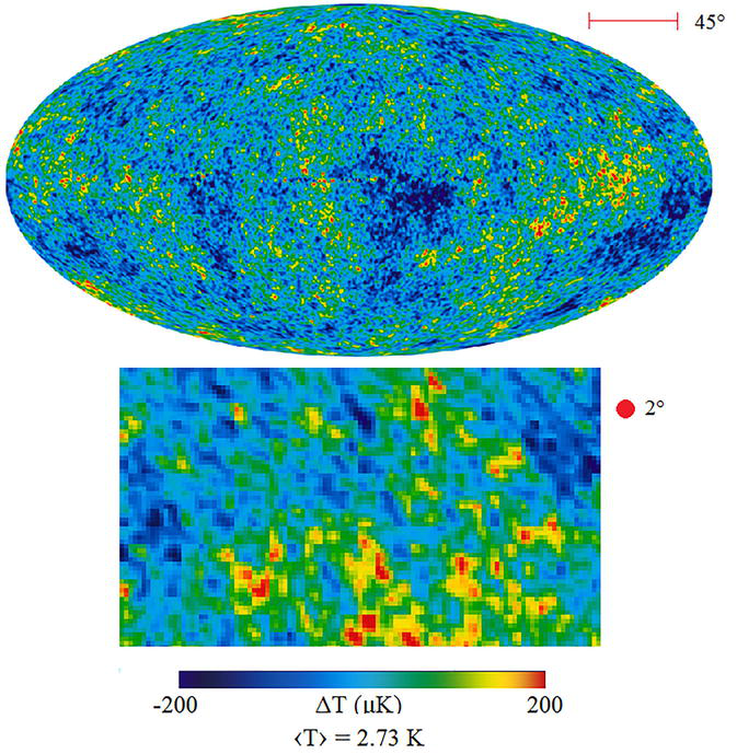
Figure 19 shows the well-known CMB anisotropy map. A portion of the map has been enlarged in the lower rectangle and two angular size references are also included.

Figure 19.

CMB anisotropy.

The CMB we receive was emitted by a spherical shell whose radius is fixed by the coordinate distance of Figure 3 when evaluated at the time of recombination, [3]. Thus, $S\left(t_{\mathit{rec}}\right)=0.6a\left(t_{\mathit{rec}}\right)$. For a structure of size, $D\left(t_{\mathit{rec}}\right)$, the subtended angle would then be

$$\theta =\frac{D\left(t_{\mathit{rec}}\right)}{S\left(t_{\mathit{rec}}\right)}\left(360/2\pi \right).$$E25

An important property of the vacuum metric is that there are no off-diagonal components linking time and the angular coordinates which means that the angle between two approaching signals does not change. This being the case, we can move this equation forward to the present day,

$$\theta =\frac{D\left(t_0\right)}{0.6a\left(t_{\mathit{rec}}\right)}\frac{a\left(t_{\mathit{rec}}\right)}{a\left(t_0\right)}\left(360/2\pi \right)=95.5\frac{D\left(t_0\right)}{a\left(t_0\right)}deg.$$E26

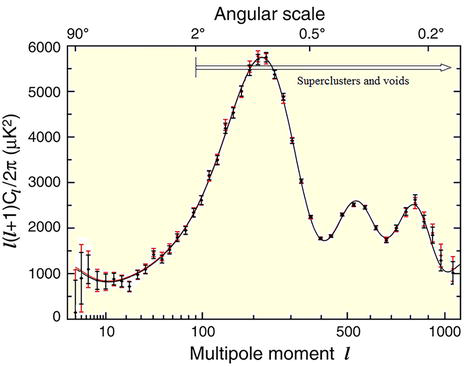
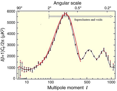
In Figure 20, we see that the first peak of the CMB spectrum has an angular size of about 1 deg.

Figure 20.

CMB spectrum.

In Table 1, we show the angular sizes of various structures and we see that superclusters (and voids) are the only structures large enough to be associated with the peak.

Object	$\theta \left(deg\right)$
Milky Way	0.0001
Groups	0.007–0.013
Clusters	0.013–0.065
Superclusters	0.2–2.0
voids	0.6–1.6
Extreme structures	> 45

Table 1.

Angular sizes of various structures.

In Figure 21, we show a plot of 71 known superclusters and voids. Using the Gaussian distribution shown, we performed a statistical calculation to determine the spectrum with the result shown in Figure 22.

Figure 21.

Count of observed superclusters (red) and voids (blue).

Figure 22.

Ensemble average supercluster/void CMB spectrum. Angles are related to the moment by $l=\pi /{\theta }_{\mathrm{rad}}=180/{\theta }_{\mathrm{deg}}$.

We find that the position of the peak is correct. The shape of the predicted peak is slightly broader than the observed peak but that is quite likely due to our assumption of spherical symmetry which is certainly not the case. The magnitude of the peak was adjusted to match the observed peak and is yet not a prediction but we do expect that a prediction will result from our new simulation mentioned previously that is still under development The second peak does not correlate with the size of any structure which is strong evidence that it is a consequence of multipole distributions within the superclusters and voids. Referring back to Figure 19, we see that the supercluster-sized structures have a range of temperatures which supports that idea.

We remind the reader that even though the superclusters have the right size, it wasn’t the superclusters per se that were responsible for the peak but rather that the process that created the superclusters simultaneously created the CMB spectrum peaks with the same dimensions.

12. Baryonic acoustic oscillations: CMB

Since this bears on the CMB anisotropy problem, this is an appropriate point to show that the baryonic acoustic oscillation model is wrong, [8]. We will first discuss the CMB issue and then the unrelated 2-point galaxy correlations model. One of the principal failings of the BAO model is that the authors assumed from the beginning that there existed a uniform distribution of radiation that needed a spectrum. We have shown, however, that that idea is simply wrong. The radiation came into existence with its spectrum in place from the beginning.

The first argument against the BAO model is simply causality. In Figure 23, we show the coordinate of a photon emitted at the time of nucleosynthesis in comparison with the coordinate size of a supercluster which we have shown has the same dimension as the spectrum peak. We see that by the time of recombination, the photon could have only traveled about 10% the distance across the supercluster.

Figure 23.

BAO causality restriction.

The second argument is concerned with the energy required to create the peaks starting from an energy source that emitted acoustic waves at the time of nucleosynthesis. At present, the relative magnitude of the CMB anisotropy is $\mathrm{\Delta }{T}_0/T_0=2\times {10}^{-4}$ and because the CMB decoupled from matter in the universe at the time of recombination, the ratio had the same value earlier at $t=t_{\mathit{rec}}$ when the temperature was 3000 K. The energy density of the anisotropy was ${\rho }_{\mathrm{\Delta }}=a_{\mathit{SB}}\left({\left(T+\mathrm{\Delta }T\right)}^4-T^4\right)=a_{\mathit{SB}}{T}^4\left(\mathrm{\Delta }T/T\right)$ which gives ${\rho }_{\mathrm{\Delta }}=4.9\times {10}^{-5}\mathrm{j}{\mathrm{m}}^{-3}$.

Also, at that time the average size of a supercluster was $4\times {10}^{21}\mathrm{m}$ so a spherical shell, with a radius of half the supercluster size and an assumed thickness equal to 10% of the radius, had a volume of $V\sim {10}^{64}{\mathrm{m}}^3$. Multiplying gives a total energy of $4.9\times {10}^{59}\mathrm{j}$. The BAO model assumes that this energy originated from a concentrated source whose size at the time of nucleosynthesis could not have been larger than $\mathrm{c}{t}_n$. The required energy density would then have been ${\rho }_{\mathrm{BAO}}=1.2\times {10}^{47}\mathrm{j}{\mathrm{m}}^{-3}$ which is $3\times {10}^{12}$ times greater than the total energy density of the universe. This argument is oversimplified but ${10}^{12}$ is a big number so it is not likely that a more sophisticated model will change the result. If one tries account for the energy by proposing a huge number of sources, one is immediately faced with the problem of specifying how to arrange, along with what did the arranging, the sources in space so that they produced the cosmic web and not some uniform distribution.

The conclusion is that baryonic acoustic oscillations on a scale needed explain the CMB spectrum are impossible.

13. Baryonic acoustic oscillations: Galaxy correlation function

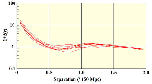
The second phenomenon attributed to BAO is the bump observed in the two-particle galaxy correlation function at a separation of $150\mathrm{Mpc}$, [8]. The existence of that bump would present a problem if BAO were the only possibility since we have argued that BAOs do not exist. There is, however, another and far simpler explanation, namely the cosmic web.

To test this idea, we built a simulation based on a cubic grid with edge lengths initially set to the average size of a supercluster. Using Gaussian statistics, we randomized the ends of the edges both in magnitude and direction according to the size distribution of superclusters. Next, we assigned a random number of galaxies to each edge with random offsets scaled by the width of a supercluster and finally, calculated the correlation function of the resulting distribution. The set of galaxies along the center grid line formed our reference set. There are a number of estimators described in the literature. The one we used is the spherically symmetric estimator given by the following (see ref. [8]),

$$1+\xi \left(r\right)=\frac{1}{N}\sum _{i=1}^N\frac{N_i\left(r\right)}{\overline{n}{V}_i\left(r\right)}$$E27

In this formula, the number of reference galaxies is N and $\overline{n}$ is the average density of all the galaxies. $N_i\left(r\right)$ is the number of galaxies lying within a thin spherical shell of radius $r$ and volume $V_i\left(r\right)$ centered on the ith reference galaxy. This ratio compares the actual number in each shell with the number expected based on the average density of galaxies. If the galaxies were distributed randomly, we would have $\xi \left(r\right)=0$.

The result of running the simulation for a number of different random number sets is shown in Figure 24. While the model is perhaps not an accurate representation of the cosmic web, the result looks very much like the observed correlation function in shape and the peak appears at the correct distance.

Figure 24.

Two-particle galaxy correlation function.

During the past two decades, a lot of effort has been spent on the galaxy correlation problem because of its potential as a standard candle for measuring distances at redshifts beyond the supernovae scale. What we have just shown is that the idea is perfectly reasonable because the coordinate dimensions of the cosmic web do not change. In all the work that has been done, one only needs to replace the wording” baryonic acoustic oscillation” with” cosmic web.”

Taken together, we have shown that BAOs are neither possible nor necessary.

14. The lithium problem

We noticed as part of our original development, [3], that certain reactions were not included in the standard BBN code and that when one in particular, ${\mathrm{Li}}^7+\mathrm{p}->{\mathrm{He}}^4+{\mathrm{He}}^4+\gamma$, was included, the predicted abundance of lithium was lower by a factor close to three. We have since come to understand, however, that missing reactions are not the most important part of the issue. We now know that the lithium problem is another issue that arises in large part because of the incorrect standard model assumption of a uniform matter distribution at the time of nucleosynthesis. We have just shown that to understand the existence of cosmic structures and the CMB, the initial densities of protons and neutrons must have varied from place to place on all length scales. The result is that the relative abundances of elements produced at any one place will vary with the location because of variations in the initial proton and neutron densities.

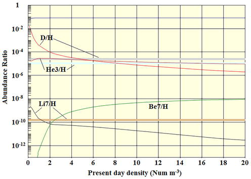
The second part of the puzzle is that the observations of the element abundances are not all taken from a single location. For example, deuterium abundances have been determined from line-of-sight observations out to distances of 100 parsecs with a result of $\mathrm{D}/\mathrm{H}=2.5\times {10}^{-5}$ but observations at much larger distances yield a value as large as $3\times {10}^{-4}$. (We note that one could with equal justification refer to the issue as the deuterium problem.) In Figure 25, we show the calculated abundances as a function of the initial baryon density, [4]. The horizontal lines are an indication of the accepted observed abundances.

Figure 25.

Nucleosynthesis abundances as a function of the initial baryon density. ${\mathrm{H}}_0=73$.

(The curves in this figure differ somewhat from those shown in [4]. The reason for this are first, that a value of $H_0=67.3$ used in [4] instead of 73 and second, that a few changes were made to the code that improves the numerical stability of the solutions for small densities. The main effect of the latter was to change the shape of the ${\mathrm{Li}}^7$ peak.)

From this figure, we see that The ${\mathrm{He}}^4$ abundance is independent of the initial density over the range considered here and consequently is only dependent on the proton/neutron density ratio. The observed ${\mathrm{He}}^4$ mass ratio is 0.245 and with $H_0=73$ we find that $\left(\mathrm{p}/\left(\mathrm{p}+\mathrm{n}\right)\right)=0.875$.

Considering now the deuterion and lithium abundances, we see that an initial baryon density of about five is necessary to match the accepted deuterium abundance but that a density of about 1 is necessary to account for the ${\mathrm{Li}}^7$ abundance so the two constraints are incompatible. We noted that measurements of the deuterium abundance in more distant regions where the initial density was lower yield a value considerably larger than the standard value and, in fact, the value $3\times {10}^{-4}$ was obtained from sources far from any galaxy (see references in [4].) Similarly, the ${\mathrm{Li}}^7$ abundance was determined from observations of low metal stars located far from the main disk of the Milky Way so a low initial density is again perfectly understandable. We also show results for ${\mathrm{He}}^3$ but since that element is very active in stars, it is questionable as to whether or not the reported abundance has any relationship to its primordial value.

We find that the new model with density variations can readily account for the observed abundances although at this point, we are not able to accurately predict the detailed initial density distribution of the Milky Way to be. The lithium problem is not a problem at all. It is only a problem if one believes that the initial baryon density was the same everywhere at the time of nucleosynthesis.

Aside from not yet being able to predict with any accuracy the initial density profile of the matter distribution of structures to be, an additional significant issue is that many of the needed reaction cross sections are not known with great accuracy. Most of the needed low energy cross sections were measured many decades ago and soon after, experimentalists moved on to higher energies. Our simulations show that choosing one data set over another can result in significant changes to the abundance curves. Our runs, however, do show that the general pattern shown in the figure remains the same. There have not been any recent efforts made to improve the situation and additional experiments are needed to fill in the gaps and resolve differences between existing cross section determinations.

15. Rotation

A long-standing although generally neglected problem in astrophysics is the source of rotation of cosmic structures. All galaxies and some galaxy clusters rotate and even though galaxies are independent entities, their rotations are not random as is evidenced by the Tully-Fisher relationship. We spoke at the beginning about the high degree of organization that exists in the universe and the rotation of galaxies is an example of that.

The standard model idea is that the infalling material during the accretion phase of galaxy development somehow managed to start the rotation. That, however, is a highly unlikely scenario because random events do not result in organized development and they certainly could not explain the correlation between the rotation rates of different galaxies.

If we assume that the rotation was initiated at the time of nucleosynthesis and that the rotation was a matter of material undergoing normal orbital motion, the rotation would have slowed as the universe expanded. But given the present-day rotation rates and working backward, we find that the initial velocities would have been orders of magnitude greater than the speed of light which is impossible. Another problem with the accretion idea is that, as we have seen, the outer regions of developing structures had no knowledge of the center until very late in their evolution which means that organizing the material into normal orbital motion could not have begun at all until sometime after the structure had evolved beyond the causality limit. By that time, however, no process could have then started the entire structure rotating.

All this indicates that the rotation is primordial. Since the rotation cannot be explained in terms of material motion, the only other possibility is that the vacuum imprint was rotating and the matter and antimatter created by the vacuum were simply carried along by the rotating vacuum. This brings us to the reality of dark matter.

16. Dark matter

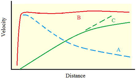
Dark matter was originally proposed to explain the motion of galaxies in galaxy clusters and later to explain the velocity distribution of the stars in spiral galaxies. Since then, it has become something of a catch-all to fix up the calculations of various cosmic phenomena that seem to defy a simple explanation.

One of the manifestations of dark matter concerns the velocity distribution of stars in spiral galaxies and the gas making up HI rings, [3, 6]. The spiral galaxy problem is illustrated by the curves in Figure 26.

Figure 26.

Typical spiral galactic velocity distribution.

The problem is that the observed distribution, curve B does not match the expected distribution, curve A. The generally accepted solution for this problem is to suppose there is a halo of dark matter surrounding the galaxy that provides the gravitation needed to match the observed velocity distribution. There are several problems with this proposal, however, not the least of which is the fact that a dark matter halo should act as a halo of stars with the lights turned off so its velocity distribution should match curve A instead of B. To get a hint about the solution, we subtract the two curves to obtain curve C and notice that it approximates the velocity profile of a rotating rigid body. What this indicates is that the observed velocity distribution of the stars can be understood in terms of some normal orbital motion riding in a rigidly rotating background.

Turning to Einstein’s equations, it is reasonable to model spiral galaxies using a stationary axisymmetric metric,

$$\begin{array}{ll}& {\mathit{ds}}^2=-A{\left(\mathit{cdt}\right)}^2+B{\left(\mathit{d\varphi }-\mathit{\omega dt}\right)}^2+{\mathit{Cdr}}^2+\mathit{Dd}{\psi }^2\\ & =-\left(A-\frac{B{\omega }^2}{c^2}\right){\left(\mathit{cdt}\right)}^2\\ & -2\frac{\mathit{B\omega }}{c}\mathit{d\psi }\left(\mathit{cdt}\right)+\mathit{Bd}{\varphi }^2+{\mathit{Cdr}}^2+\mathit{Dd}{\psi }^2\end{array}$$E28

with an energy-momentum tensor of the form

$${\mathbf{T}}^{\mathit{\mu \nu }}=\left({\rho }_{\mathit{vac}}{c}^2+p_{\mathit{vac}}\right)\frac{u^{\mu }{u}^{\nu }}{c^2}+p_{\mathit{vac}}{\mathbf{g}}^{\mathit{\mu \nu }}+{\rho }_m{c}^2\frac{v^{\mu }{v}^{\nu }}{c^2}.$$E29

A small volume of the vacuum will respond to the total gravitation field in the same way as a material particle which means that we can analyze its motion using the usual geodesic equations. The first two of these are satisfied identically as a consequence of our assumption of a stationary metric. The remaining two have the solution

$${\dot{\phi }}_{\mathit{vac}}\left(r,\psi \right)=\omega \left(r,\psi \right)$$E30

where $\omega \left(r,\psi \right)$ represents the rotation of the galaxy. We find that the vacuum must rotate and, as shown in [3], it must do so with zero angular momentum. Because of that fact, the rotation is not subject to the slowing induced by the expansion as would be normal orbital motion.

We now consider the stars whose velocity must also satisfy the geodetic equations. We separate their motion into a component that is at rest in the vacuum, and hence without angular momentum, and a residual with normal orbital motion, ${\dot{\varphi }}_m={\dot{\varphi }}_{m,r}+\overline{\omega }$. Solving the geodetic equations gives

$${\dot{\varphi }}_{m,r}\left(l,z\right)=\frac{v}{l}-\overline{\omega }\left(l,z\right)$$E31

which exhibits the behavior shown in Figure 26. On the left is the normal orbital rotation, curve A, the first term on the right is the constant velocity component, curve B, and the second is the rigid body vacuum rotation, curve C. At the outer edge of the galaxy, the constant stellar velocity $v=\overline{\omega }\left(l_G,0\right)$ equals the rotation rate so ${\dot{\varphi }}_{m,r}\left(l_G,0\right)=0$ which means that the outermost stars are at rest in a rotating vacuum.

This result dovetails quite nicely with the rotation model discussed in the previous section. In that case, the vacuum rotation carried along the material and, in this case, the material appears to drag along the vacuum but the result is the same. The vacuum rotation is a consequence of the Planck era imprint but it is likely that the residual orbital motion did not begin until after the ZVPs were reached and the galaxies began to collapse.

Another problem mentioned in [1] is known as the “angular momentum catastrophe.” The idea behind this thoery is that the development of disk galaxies, and in particular their sizes, can be understood in terms of their angular momenta [9]. The problem is that the theory does not work. The predicted sizes are an order of magnitude too small. There are a number of assumptions made that we do not accept such as the idea that their rotations are a consequence of tidal torques between neighboring galaxies instead of being primordial. The reason for that is that gravitation had no effect on the evolution of galaxies until very shortly before they began their initial collapse and certainly could not have exerted enough torque on neighboring galaxies to start them rotating within the short time interval prior to their ZVP. All galaxies rotate and it is highly unlikely that this mechanism could account for their rotations considering the variations in their separations and orientations. The reason for putting these comments in this section, however, concerns the assumption that the angular momentum of the stars increases with distance from the center of the galaxy. In this new model the exact opposite is true. The outer stars in a disk are carried along by the rotation of the vacuum and do not have any angular momentum at all.

In the references, we discuss other cases in which vacuum energy is shown to account for phenomena attributed to dark matter. Summing up, when the vacuum is included in Einstein’s equations, the dark matter problem disappears.

17. Hubble tension

During the past two decades or so, a lot of effort has gone into the problem of pinning down the value of the Hubble constant. The various methods can be grouped according to the redshift range involved. First are those based on observations in the range from about 0.01 to an upper limit of 6 or so. The significance of the lower limit is that it is the smallest redshift for which the recession velocities of galaxies have a reasonable probability of being significantly larger than their peculiar velocities. The upper limit just represents the time of galaxy formation. The Hubble constant determined by methods covering this range is settling on a value of $H_0\approx 73$, [8].

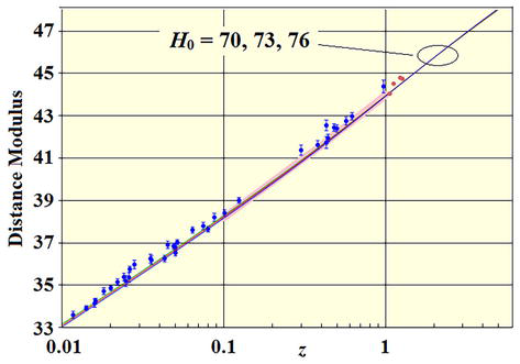
In Figure 27, we show new model luminosity distance modulus predictions for 3 values of the Hubble constant. As we see, there is only a very slight dependence on the Hubble constant. It is important to appreciate that the new model has no other adjustable parameters and that varying the Hubble constant changes the result hardly at all so a failure to fit the data would be a real problem for the model. It appears that the model predictions lie a little below the data points but the figure shows only a very limited number of the total number of data points now in existence. When the new points are included, the new model fit is extremely good.

Figure 27.

Luminosity distance predictions of the new model. Refer to [3] for a detailed description of the data points.

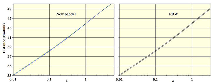
We now compare with the $\mathrm{\Lambda CDM}$ predictions which are shown in Figure 28. We see that the $\mathrm{\Lambda CDM}$ model shows a greater dependence on the value of the Hubble constant than does the new model. The predictions of the two models are, however, in no way of equal significance. As already noted, the new model prediction cannot be adjusted. The $\mathrm{\Lambda CDM}$ model results, on the other hand, aren’t predictions at all but instead are curve fits with three parameters; ${\mathrm{\Omega }}_m$, ${\mathrm{\Omega }}_{\mathrm{\Lambda }}$, and the Hubble constant.

Figure 28.

Model and FRW predictions for $H_0=70$ and $H_0=76$. The FRW parameters are ${\mathrm{\Omega }}_m=0.3$ and ${\mathrm{\Omega }}_{\mathrm{\Lambda }}=0.7$.

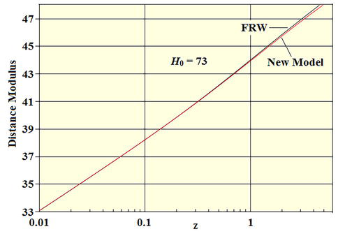
The Riess SHOES group finds a value of $H_0=73.3$ for the FRW parameters just indicated. In Figure 29 we see that with $H_0=73$, the results are essentially identical for redshifts somewhat smaller than two. Since the value $H_0=73$ gives the best fit of the data in the $\mathrm{\Lambda CDM}$ case, it validates the prediction of the new model.

Figure 29.

New model (red) and FRW (black) predictions for $H_0=73$.

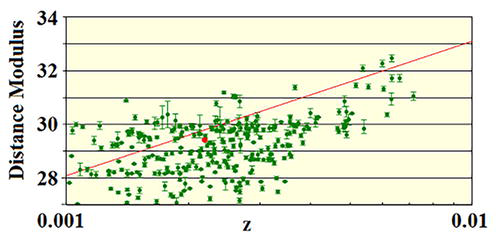
The second grouping of methods covers the redshift range from 0.01 down to some lower cutoff which we will take to be 0.001. The overriding factor in this redshift range is that the galactic pecular velocities are as large or larger than the recession velocities. The best-known results covering this redshift range are those of the Tip of the Red Giant Branch (TRGB) group. They claim that their data results in a Hubble constant of $H_0=69.8$ which comprises the second largest contributor to the Hubble tension. There are, however, problems with that result. First, the sample set used contained only 18 galaxies, and second, the results are very sensitive to the statistical model used to separate the recession velocity of each galaxy from its observed velocity.

In [8], we did a fit using all the data points in the TRGB database that had observed velocities in the redshift range we are considering. The result was a total of 291 galaxies. To determine the Hubble constant, the recession velocity of each galaxy has to be separated from the observed velocity and at present, the only way this can be done is by using a statistical model which is based on the mass distribution of the local universe. Tools that implement this process are available online in the Extragalactic Distance Database, https://edd.ifa.hawaii.edu/ which also contains the TRGB database.

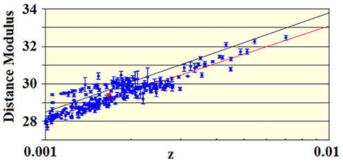
In Figure 30, we show the raw data points and in Figure 31, the same set corrected for the peculiar velocities using the probabilistic model. The red line is the new model prediction. The difference between the two distributions makes it obvious that the peculiar velocities are large so any prediction made is highly dependent on the accuracy of the correction.

Figure 30.

TRGB raw data points.

Figure 31.

TRGB data points adjusted for peculiar velocities.

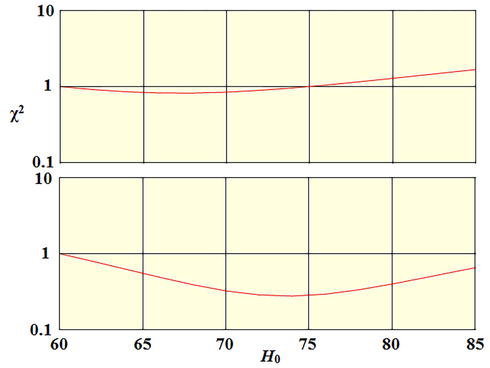
If the model were completely accurate, all the adjusted data points would lie along a single line. Since they do not, there is obviously a problem. We note that the new model prediction gives a good fit to what appears to be the correctly adjusted galaxies. In Figure 32, we show normalized ${\chi }^2$ results for two cases. In the upper panel, we show the result for the full data set of Figure 30. This indicates a Hubble constant in the range 66–67 which is not a lot different from the group’s published value. In Figure 31, we have included a black line that roughly separates the spurious points from the primary set. In the lower panel of Figure 31, we show the result when the data points above the black line are removed. This time the result is a Hubble constant close to 73 in agreement with the supernovae determinations so clearly, it is the peculiar correction model that is being tested rather than the distance determinations and with perfect corrections, there would not be any tension.

Figure 32.

${\chi }^2$ for the data points in Figure 31. The upper panel is the result with all the data points included and the lower panel with the points above the black line removed.

The third redshift grouping, commonly referred to as cosmological, groups together those methods covering redshifts greater than that of galaxy formation. The BAO model of the CMB spectrum falls under this heading and it is the only such model making a Hubble constant prediction. The consensus value is $H_0\approx 67$ which constitutes the biggest portion of the Hubble tension. We have already shown, however, that the BAO model is wrong so this Hubble constant value can be dismissed.

There are other approaches such as the Megamaser and $L-\sigma$ methods which are discussed in [8]. The results from those two methods are consistent with a value of 73. Still other methods are discussed in [1].

There is one further approach that has the potential for becoming a viable method for determining the Hubble constant. The idea is to measure the rate of recession of bodies within the solar system. At present, there is considerable interest in Moon-Earth distance because 70 years of accurate distance measurements already exist. Calculating the Hubble flow contribution to the total recession rate is very simple and the result shows that the rate is well within a range that can be measured. The difficulty comes from the fact that all the other contributors to the Moon’s recession, in particular the tidal effects, must be determined with an combined error of no more than 1 or 2 percent before a Hubble determination can be made.

Planetary recession offers other opportunities. Instead of the 3.8 cm per year recession of the Moon, the rates would be 10 meters per year or more depending on the planet. Measuring the distance becomes more difficult but, on the plus side, the planets are not as subject to the large tidal effects that make the Moon determination difficult.

Summing up, of the two principal contributors to the tension, one is just wrong and the other did not include the entire data set or properly make allowances for errors in the peculiar velocity prediction model. When the spurious values are removed, the results yield the same value as that of the larger z studies. The conclusion is that the tension has been eliminated and the correct value is very close to $H_0=73.$

18. Tying things together

We have shown that accretion initiated by small fluctuations in an otherwise uniform distribution of ordinary matter is impossible. We also showed that gravitation was ineffective until shortly before $t_G$ so the idea that accretion is the primary source of cosmic structures is wrong. Another insurmountable problem with accretion is that no process that involves communication could account for structures as large as superclusters. The conclusion we reached is that the existence of structures is a consequence of an imprint established during the initial Planck era inflation. Since the imprint regulated the material manifestation of the structures at the time of nucleosynthesis, Figure 19 is not just a map of the CMB anisotropy but is also a photograph of the vacuum as it existed at the end of the inflation.

This, however, leaves us with the question of what organized the imprint. It could not have been some random process so there must have been some rule that regulated its development. We know that causality played no part in the development and that whatever the rule was, it must have been extremely simple. In terms relative to the size of the expanding universe, the imprint structures ranged from the size of a star up to the size of superclusters with the latter being nearly as large as the universe at the end of the inflation and the beginning of the transition. The energy densities of these structures, on the other hand, were on the order of ${10}^{-4}-{10}^{-5}$ relative to the average so they were large but faint.

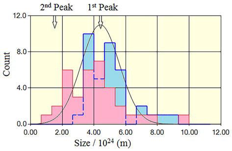
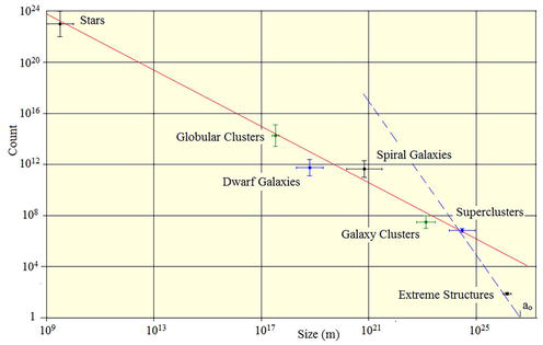
In Figure 33, we show a plot of the count of cosmic structures versus their size, [3].

Figure 33.

Count of structures vs. size.

What is remarkable is that aside from the extreme structures, all cosmic structures with their vast differences in size and numbers lie on a power-law curve and this holds all the way down to the stars. The extreme structures (size $>{45}^{\circ }$) fall below this line but this is simply a consequence of the finite size of the universe. Another point to notice is that the structures have distinct sizes with no overlap. If accretion was the process by which the structures were formed, one would expect a continuum of sizes instead. A fit to the curve has the following result

$$C\left(s\right)=5.7\times {10}^6{\left(\frac{s_{\mathit{sc}}}{s}\right)}^{1.1}$$E32

where we have scaled by the average size of a supercluster. The dashed line shows the count of structures of a given size that would fill the universe and its formula is

$$C_{\mathit{\text{filled}}}\left(s\right)={\left(a_0/s\right)}^3.$$E33

We see that superclusters fall on both lines so, in an order of magnitude sense, they fill all space.

The significant factor in the second formula is the power of three. The idea of a fractal dimension extends this concept to situations in which the power can have any value, not just an integer but this is exactly the form of (Eq. (32)) so we find that the structure imprint had a fractal dimension of about 1.1. It is generally true that the fractal dimension of any system is larger than the geometric dimension of that same structure so it follows that the cosmic structure must be 1-dimensional or in other words, that the structure of the universe must be one of filaments which gives us the cosmic web.

A defining property of fractal structures is self-similarity and this suggests that self-similarity was in some way the defining principle that regulated the formation of the imprint.

19. Conclusions

We have summarized the results contained in a series of papers published during the past 3 years. A new model of cosmology based on a universe with time-varying curvature is presented that makes a large number of predictions that agree with observation. This model includes a new model of nucleosynthesis that accounts for the existence of all cosmic structures and the CMB, the origin of galactic supermassive black holes, and the stability of galaxy clusters. It also explains the existence of very large galaxies at a time at which the standard model says they could not yet exist.

We have shown that the problems with the standard model boil down to three incorrect assumptions and one omission; the first incorrect assumption is that the curvature of spacetime is constant, the second is that the initial distribution of matter was uniform, and the third is that structure formation was a results of accretion. When those assumptions are abandoned and vacuum energy is included in the energy-momentum tensor, everything falls into place.

Here at the end, we are back at the beginning with two problems to solve. The first is to understand the evolution of the Planck era inflation. We have no clear idea of how the fractal imprint came into existence but we have demonstrated that it was responsible for the universe we observe. The second problem is to understand the breaking of the baryon conservation law that results in the creation of the very small percentage of extra neutrons at the time of nucleosynthesis.

References

1.Perivolaropoulos L, Skara F.. Challenges for ΛCDM: An update. arXiv:2105.05208v3. 6 Apr 2022
2.Abdalla E, et al. Cosmology intertwiined: A review of the particle physics, astrophysics, and cosmology associated with the cosmological tensions and anomalies. arXiv:2203.06142vf1. 2022
3.Botke JC. A different cosmology - thoughts from outside the box. Journal of High Energy Physics Gravitation and Cosmology. July 2020;6(3):473-566
4.Botke JC. The origin of cosmic structures part 4 – nucleosynthesis. Journal of High Energy Physics, Gravitation and Cosmology. 2022;8(3):768-799
5.Botke JC. The origin of cosmic structures part 1 - stars to superclusters. Journal of High Energy Physics, Gravitation and Cosmology. 2021;7(4):1373-1409
6.Botke JC. The origin of cosmic structures Part 2 - HI rings. Journal of High Energy Physics, Gravitation and Cosmology. 2021;7(4):1410-1424
7.Botke JC. The origin of cosmic structures Part 3 - Supermassive black holes and galaxy cluster evolution. Journal of High Energy Physics, Gravitation and Cosmology. 2022;8(2):345-371
8.Botke JC. The origin of cosmic structures Part 5 - Resolution of the hubble tension problem. Journal of High Energy Physics, Gravitation and Cosmology. 2023;9(1):60-82
9.van den Bosch F, C, Burkert A, Swaters RA. The angular momentum content of Dwarf galaxies: New challenges for the theory of galaxy formation. Monthly Notices of the Royal Astronomical Society. 2001;326(3):1205-1215
Written By
John C. Botke
Submitted: 23 June 2023Reviewed: 27 June 2023Published: 22 July 2023