Recent Advances on Image Edge Detection

Abstract

This chapter delves into the intricate field of image edge detection, a pivotal aspect of computer vision and image processing. It provides a comprehensive exploration of the underlying principles, methodologies, and algorithms employed in the identification and extraction of significant contours in digital images. Traditional edge detection techniques, as well as advanced approaches that are based deep learning, are thoroughly examined.

1. Introduction

In the world of computer vision and image processing, edge detection plays a fundamental role. Edge detection techniques enable computers to identify and extract important boundaries and contours from digital images, leading to numerous applications such as object recognition, image segmentation, and feature extraction.

Many research works have been conducted on this sense. In Ref [1], Ziou and tabbone proposed an edge detection algorithm based on the Robert operator introduced by Lawrence Roberts in 1963—a rudimentary yet pioneering step in the field. In Ref [2], Shrivakshan and Chandrasekar used the Prewitt operator, tailored for scenarios with high noise and fading pixel values. Then, Sobel operator [3]-based algorithm was proposed [4] and have given the differentiation algorithms a particular popularity. Xin Wang used then the Laplacian operator [5], leveraging second-order differentiation for more precise edge identification. In a significant milestone, John Canny introduced the optimal Canny operator [6]. This method continuously improved image contour information through a series of filtering, enhancement, and detection steps, ushering in a new era and establishing higher standards in the field of edge detection.

The previous mentioned differentiation approaches are now considered as traditional. In fact, with the progress of artificial intelligence, a lot of recent research has focused on edge detection and proposed deep learning-based approaches. In Ref. [7], Bertasius proposed (DeepEdge), a two branches-based deep network for edge detection. In the first one, a classification solution is applied to predict the edge likelihood. In the second one, regression criteria to predict edges based on training data. By combining multi-scale levels, Xie and Tu proposed the HED, a holistic nested edge detection [8] that can predict hierarchical representations. In Ref. [9], Deng et al. enhanced the HED using the VGG16 [10] as a backbone network and implementing a full convolution architecture. The solution named, LPCB, avoids some prediction ambiguities as thick edges allowing better detection performance. In Ref. [11], Yang et al. proposed a full convolution codec network ECDN. Such network includes a decoder through deconvolution steps aiming at resizing the encoder output map to the original image size. The decoder allows better edge localization performance. Since complexity is also a key point, Su et al. have proposed lightweight architecture named Pixel Difference Network (PiDinet) [12]. In this proposal, the authors integrate a differential operator into the network to perform a novel pixel difference convolution. In Ref. [13], Xavier Soria differentiates between edges, contours, and boundaries and consider them as three distinct visual features and propose two sub-networks: Extremely Dense initial network and an Up-sampling part. In Ref. [14], Elharrouss propose the (CHRNet) network where he maintains the high-resolution of the edge map during the network stage overcoming the down-sampling of pooling and connect consecutive scales through sub-blocks. Due to the complexity of the proposed networks, some research proposed a light-weighted solutions as in Ref. [15].

The rest of the chapter is organized as follows. First, we present in basics of image detection, edge types, applications, used dataset, and evaluation criteria in Section 2. Then, we discuss the traditional edge detection methods in Section 3. In Section 4, we describe the basics of recent deep learning-based approaches and present our conclusions in Section 5.

2. Basis of image edge detection

2.1 Definition of image edges

In the domain of digital imagery, an edge encapsulates a fundamental concept embodying the transition between contrasting regions within an image. Specifically, an edge marks the boundary where intensity or color values undergo significant and rapid changes. These variations might indicate shifts in texture, object boundaries, or underlying structures in texture area. Mathematically, an edge can be seen as a locus of points where the derivative of spatial intensity (Luminance) or color (chrominance) experiences a pronounced variation. Figure 1 illustrates the edge lines in white color.

Figure 1.

Detected edges.

2.2 Types of edges

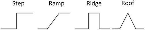
Edges in images exhibit diverse characteristics based on the nature of the underlying transitions in intensity or color. These variations lead to the classification of edges into several distinct types as presented in Figure 2, each conveying different information about the image content.

Figure 2.

Types of edges.

2.2.1 Step edges

Step edges are perhaps the most fundamental type of edge, characterized by a sudden and significant change in intensity across neighboring pixels. These transitions often correspond to object boundaries or abrupt changes in surface orientation. Step edges manifest as sharp transitions, representing a rapid shift from one color or brightness level to another.

2.2.2 Ramp edges

Ramp edges denote a smoother transition in intensity, typically resembling a linear change across adjacent pixels. This type of edge can arise from gradual shifts in illumination or material properties, such as the transition from a shadowed region to a well-lit area.

2.2.3 Ridge edges

Ridge edges represent situations where the intensity undergoes a gradual decrease before experiencing a sudden increase. This type of edge is prominent in scenarios where a transition from a brightly illuminated region to a shadowed area takes place, creating a ridge-like intensity profile.

2.2.4 Roof edges

Roof edges are characterized by a transitional phase that exhibits a gradual increase in intensity followed by an abrupt decrease. These edges often occur in images with highlight reflections or transition from shadow to highlight regions.

Understanding the different types of edges is essential, as they provide insights into the underlying content of an image. Recognizing the specific type of edge can aid in accurately interpreting the objects, materials, or lighting conditions present within the image. This categorization forms the basis for subsequent edge detection methodologies, enabling the development of techniques tailored to different edge types.

This pixel based classification based is mainly significant for traditional edge detection approaches, which will be addressed in next sections.

2.3 Applications of edge detection

Edge detection, a foundational technique in image processing and computer vision, demonstrates its significance through various applications and disciplines:

1. Image Segmentation: Edge detection frequently precedes image segmentation, delineating images into coherent regions. Edges play a pivotal role in distinguishing objects and structures.

2. Object Detection and Recognition: In identifying and recognizing objects, edge detection defines their contours, enabling subsequent classification and analysis.

3. Medical Imaging: Edge detection finds utility in medical imaging, delineating organs, vessels, and anomalies within X-rays, MRI scans, and CT images, augmenting diagnostic accuracy.

4. Robotics and Autonomous Systems: Essential for real-time processing, edge detection empowers robots and autonomous vehicles to navigate, discern obstacles, and interpret visual inputs.

5. Biometrics: In biometrics, edge detection distinguishes intricate patterns in fingerprint recognition and retinal scans, allowing better identification accuracy.

6. Document Analysis: Edge detection helps analyze documents, character recognition, processes forms, and extracts textual content.

7. Satellite Image Processing: In satellite imagery, edge detection aids in landform assessment, urban monitoring, and environmental analysis.

8. These diverse applications underscore edge detection’s pivotal role in extracting crucial insights from images, underpinning sophisticated image analysis across an array of scholarly disciplines.

3. Traditional edge detection techniques

Gradient-based edge detection techniques are cornerstone approaches in identifying abrupt changes in intensity across an image. These methods exploit the concept of gradient, which represents the variation of intensity at each pixel position. By locating areas with high gradient values, gradient-based methods can effectively locate edges.

3.1 Roberts operator

The Roberts operator [1] uses a pair of simple 2x2 kernels to compute the gradients along the diagonals. It is relatively simple to implement in comparison with other operators. However, it is sensitive to noise due to its small kernel size.

3.2 Prewitt operator

Similar to the Roberts operator, the Prewitt operator [2] employs convolution but with specific 3x3 kernels to calculate gradients along both horizontal and vertical directions. The absolute magnitude of these gradients helps detect edges.

3.3 Sobel operator

The Sobel operator [3] is a widely employed gradient-based technique for edge detection. Like the Prewitt operator, it utilizes convolution with two 3x3 kernels, one for detecting horizontal edges and the other for vertical edges. The resultant gradient magnitude and direction provide insights into the edge’s strength and orientation.

3.4 Laplacian of Gaussian (LoG)

The Laplacian of Gaussian (LoG) [5] is a prominent edge detection technique that combines the benefits of smoothing and gradient-based approaches. This method involves two key steps: applying Gaussian smoothing and then calculating the Laplacian operator.

Gaussian smoothing: The first step of LoG is to convolve the image with a Gaussian kernel. Gaussian smoothing reduces noise and emphasizes areas with significant intensity changes, effectively highlighting potential edges.

Laplacian operator: The Laplacian operator is then applied to the Gaussian-smoothed image. It computes the second derivative of intensity, highlighting regions where the intensity changes rapidly. This operation enhances edges while suppressing gradual intensity variations. Combining Gaussian smoothing and the Laplacian operator helps LoG overcome noise-related issues in gradient-based methods. However, LoG may also lead to over-detection of edges and generate multiple responses for a single edge due to the nature of the Laplacian operator. Consequently, techniques like zero-crossing detection are employed to refine the edge map and extract accurate edges from the enhanced image.

3.5 Canny edge detection

Canny edge detection [6] is a multi-step algorithm widely recognized for its effectiveness in accurately identifying edges while suppressing noise. Developed by John F. Canny in 1986, this method aims to optimize edge detection by addressing the disadvantages of earlier techniques.

Gaussian smoothing: Canny edge detection begins with applying Gaussian smoothing to the image. The Gaussian filter reduces noise and creates a smoothed representation of the image, which is crucial for accurate edge detection.

Gradient calculation: This step involves computing the derivatives of the smoothed image in both the horizontal and vertical directions. The gradient magnitude highlights regions with significant intensity changes, indicative of edges, while the gradient direction provides the edge orientation.

Non-maximum suppression: Non-maximum suppression eliminates false detection in the gradient magnitude image by thinning edges. It consist in preserving only the local maxima along the direction of the gradient.

Hysteresis thresholding: Hysteresis thresholding is the final step, classifying pixels into strong, weak, or non-edges. This step employs two threshold values: a high threshold to identify strong edges and a low threshold to detect weak edges. Weak edges are retained only if they are connected to strong edges.

The Canny edge detection algorithm produces sharp, well-defined edges while also handling noise effectively. Its adaptability through parameter tuning makes it suitable for various image types and conditions. However, setting appropriate thresholds can be challenging, and the algorithm’s multi-step nature may impact its computational efficiency. Despite these considerations, Canny edge detection remains an effective technique in image processing due to its balance between accuracy and noise robustness.

4. Deep learning-based edge detection

Deep learning represents a significant progression within machine learning, especially in image processing.

The key point is its foundation in neural networks—layered algorithms inspired by the human brain’s neural structure. This emulation empowers machines to learn more effectively than traditional machine learning models. Many deep learning-based research works rely on backbone networks, a kind of network architectures. Then, elucidating theses essential concepts is pivotal for comprehending primary approaches within edge detection.

4.1 Concept of neural network

A neural network is a computational model inspired by the structure and function of the human brain’s interconnected neurons.

It consists of interconnected nodes, or “neurons,” organized into layers. These networks are designed to process and interpret complex patterns and relationships in data.

A typical neural network includes an input layer, one or more hidden layers, and an output layer. Neurons in each layer are connected to neurons in adjacent layers through weighted connections. These weights determine the strength of the connections, enabling the network to learn from data and adjust its internal parameters during a training process. Neural networks excel in tasks such as pattern recognition, classification, regression, and feature extraction. Their capacity to learn from large amounts of data and discover intricate patterns makes them especially suitable for complex problems in fields like image.

4.2 Convolutional neural network

Convolutional Neural Network (CNN) is the main key point in deep learning-based edge detection. A CNN is a type of neural network specifically designed for processing and analyzing visual data, such as images and videos.

Indeed, CNNs play a central role in the field of computer vision by revolutionizing how machines perceive and analyze images.

Some of the main roles of CNNs are as follows:

• Feature Extraction

• Image Classification

• Object Detection

• Image Segmentation

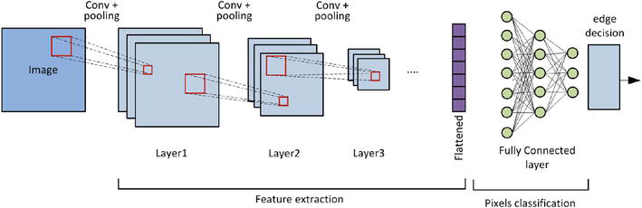
At its core, a CNN is composed of multiple layers that perform various operations on the input data. A typical CNN architecture is exposed in Figure 3.

Figure 3.

A typical CNN architecture.

The CNN components include the following:

1. Input Layer: This is the raw image data, considered as the input into the network. Images are represented as a grid of pixel values.

2. Convolutional Layer: This layer applies filters (also called kernels) to the input image. It aims to extract specific features such as edges, corners, or textures. The filters slide across the image, performing convolutions and generating feature maps.

3. Pooling Layer: Also known as subsampling or downsampling, this layer reduces the spatial dimensions of the feature maps. It helps reduce computational complexity and makes the network more invariant to small variations in position.

4. Fully Connected Layer: Toward the end of the network, one or more fully connected layers aggregate the extracted features and make decisions. In image classification, these layers connect to the output neurons representing different classes.

5. Flattening: Before the fully connected layer, the 3D feature maps are flattened into a 1D vector. This allows them to be connected to the fully connected layer.

6. Output Layer: The final layer produces the network’s output. In image classification, this might be a softmax layer that assigns probabilities to different classes.

7. Loss Function: The loss function quantifies the difference between the predicted output and the true labels. It serves as a guide for adjusting the network’s weights during training.

8. Backpropagation: The network adjusts its internal parameters (weights and biases) using backpropagation. The gradients of the loss with respect to the weights are calculated and used to update the weights through optimization algorithms like Stochastic Gradient Descent (SGD).

9. Training: The network is trained using labeled data, where it iteratively adjusts its parameters to minimize the loss function. The training data help the network learn to recognize features and patterns.

10. Prediction: After training, the network is evaluated on unseen data to assess its performance. It is then used to make predictions on new, unseen images.

11. The above steps constitute a basic overview of how a CNN operates. Depending on the architecture and specific task, the network’s structure and the number of layers may vary.

4.3 Backbone networks

In image processing, backbone networks refer to the foundational architectures that serve as the initial configurations of deep neural networks designed for tasks such as image analysis, object recognition, and segmentation.

They serve as the foundation upon which more specialized architectures and algorithms are built to perform various image processing tasks effectively. The most popular backbone are VGGs, ResNets, and Inception v1—GoogleNet.

4.3.1 AlexNet

AlexNet [16] is a pioneering CNN architecture that achieved remarkable success in the ImageNet Large Scale Visual Recognition Challenge (ILSVRC) competition in 2012. Developed by Alex Krizhevsky, Ilya Sutskever, and Geoffrey Hinton, AlexNet marked a significant breakthrough by employing deep learning techniques for image classification tasks. Notably, AlexNet consisted of eight layers, including five convolutional layers and three fully connected layers. This design was substantially deeper than previous models and facilitated the recognition of intricate features in images. AlexNet’s success was further propelled by the utilization of Rectified Linear Units (ReLU) as activation functions, dropout for regularization, and the novel implementation of Graphics Processing Units (GPUs) for accelerated training. It demonstrated the potential of deep neural networks in image classification tasks, inspiring subsequent developments of more high-performing architectures.

4.3.2 VGGs

VGG16, denoting the VGGNet model [10], represents a convolutional neural network (CNN) architecture comprising 16 layers. Its appellation originates from “Visual Geometry Group.” Proposed by K. Simonyan and A. Zisserman from Oxford University, this model has notably excelled in the ImageNet dataset, achieving a remarkable test accuracy of 92.7%. Positioned prominently in the ILSVRC-2014 competition, VGG16 stands as a remarkable achievement.

4.3.3 ResNet

In 2015, the deep residual network (ResNet) [17] emerged as an important contribution in the domain of computer vision and deep learning.

It is particularly recognized for the ability to facilitate training of networks encompassing hundreds, or even thousands, of layers while sustaining compelling performance.

ResNet introduced the innovative concept of an “identity shortcut connection.” This mechanism enables the model to bypass one or more layers, facilitating training on extensive layer configurations without compromising performance. ResNet has gained prominence as a leading architecture in diverse computer vision tasks beyond image classification, including object detection and facial recognition, owing to its robust representational capacity.

4.4 Supervised learning-based edge detection

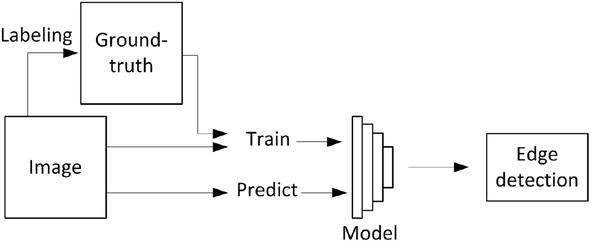
Supervised learning in image edge detection is a machine learning approach where algorithms are trained to identify and classify the boundaries or edges. The key point in such approach is the rely on a labeled dataset used to train the model. A process flow of supervised learning edge detection is presented in Figure 4.

Figure 4.

Supervised learning approach.

This approach involves the following key steps:

1. Labeled Edge Data: In supervised edge detection, we have a dataset consisting of images as input data and corresponding labels or annotations that indicate the locations of edges or boundaries within these images. The labels specify which pixels or regions in the images are part of an edge. In general, the labelling process is done manually and its output is the called ground truth. This ground-truth information serves as a reference for evaluating the performance of edge detection algorithms.

2. Training Phase: During the training phase, the algorithm uses this labeled image data to learn the relationships between the visual features in the images and the locations of edges. It aims to create a model that can accurately identify these edges within new, unlabeled images.

3. Feature Extraction: Image features, such as gradients, intensity changes, or other relevant characteristics, are extracted from the input images. These features serve as the basis for the algorithm to make edge predictions.

4. Prediction of Edges: Once the model is trained, it can be used to analyze and predict the edges on new images.

The CNN-based supervised learning approaches are hardly categorizable, as many works combine many techniques. We separate here the approaches based on two main techniques: codec-based and multi-scale fusion-based techniques. But it is not impossible to find a research work that combines these techniques for refinement purpose.

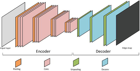
The codec-based technique is quite related to the property of the CNN itself. In fact, due to the downscaling effects of convolutional networks through successive convolutions and pooling, the ultimate output does not correspond to each pixel in the initial image. To address this, a decoder is added after the encoding. A representative process of the codec-based edge detection is presented in Figure 5.

Figure 5.

The architecture of the codec-based edge detection.

While the encoder network’s role is to generate semantic-rich feature images, the decoder task is to up-sample these low-resolution feature images through de-convolutions. The goal is to remap feature images, to match the input image’s dimensions for pixel-level matching.

Among the research works in this context, we can mention CEDN [11], CASENet [18], REDN [19], and RINDNet [20].

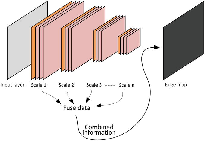
The multi-scale fusion-based technique presented in Figure 6 is related to another property of CNN. In fact, this later operates in a layer-by-layer extraction of target features, a process in which the concept of perceptual field assumes critical importance. Notably, higher layers exhibit an expanded perceptual field, facilitating robust semantic characterization, while lower layers, with a smaller perceptual scope, excel in extracting geometric details.

Figure 6.

Multi-scale typical architecture-based edge detection.

Then fusing multi-scale features enables it to capture both fine-grained details and broader contextual information simultaneously.

This approach, consisting in the integration of features across divergent scales, emerges as a pivotal modality for substantial enhancement in the research work on edge detection. Among the works in this sense, we can find DeepEdge [7], HED [8], LPCB [9], PidiNet [12], DexiNed [13], RCN [21], and DSCD [22].

We can summarize a comparison between the two approaches as follows:

• Codec-based algorithms:

  • Advantage: Better edge pixel-to-pixel localization on the output map avoiding the low resolution of pooling process.

  • Disadvantages: The decoder approximately doubles the complexity of the network

• Multi-scale fusion-based algorithms:

  • Advantage: Better combination of semantic information extracted from higher layers and the geometric details extracted from lower layers.

  • Disadvantages: Processing of many inter-layers parameters can increase complexity

5. Edge detection performance evaluation

5.1 Evaluation criteria

Evaluation criteria for edge detection techniques serve as benchmarks to assess the performance and efficacy of various algorithms. The most common metrics in recent research works are Optimal Dataset Scale (ODS) and Optimal Image Scale (OIS). But there are many other related metrics that should be considered. We present here the main common evaluation metrics used in edge detection:

1. Precision: Precision measures the ratio of correctly detected edges to the total number of detected edges.

2. Recall, also known as sensitivity, calculates the ratio of correctly detected edges to the total number of actual edges in the image.

   It is common to present a Precision-Recall Curve. This curve illustrates the relationship between precision and recall across various threshold values, offering information into an algorithm’s performance across different operating parameters.

3. F-score: This F-score [23] is a combination of precision and recall, providing a balanced assessment of algorithms performance in terms of both false positives (false-detected edges) and false negatives (non-detected edges).

$$F-\mathit{\text{scrore}}=\left(1+p^2\right)\times \frac{\mathit{Pr}\times R}{p^2\times \mathit{Pr}\times R}$$E1

Where p is a threshold value, Pr being the precision and R is the recall. Adjusting the threshold allows us to refine on the impact of precision and recall.

1. ODS (Optimal Dataset Scale): This metric represents the optimal F-score obtained at a fixed threshold for the whole dataset.

2. OIS (Optimal Image Scale): OIS is obtained from the F-score by finding the best threshold for each image in the dataset.

3. Accuracy: Accuracy evaluates the overall correctness of edge detection results, considering both true positives (correct detected edges) and true negatives (correct detected non-edges).

4. Mean Squared Error (MSE): MSE computes the average squared difference between the detected edges and the ground truth edges (The ground truth is a contours generally drawn by humans and used to evaluate the edge detection algorithms. Lower MSE values indicate better edge detection accuracy.

5. Mean Absolute Error (MAE): MAE calculates the average absolute difference between detected and ground truth edges. Similar to MSE, lower MAE values signify more accurate edge detection.

6. Receiver Operating Characteristic (ROC) Curve: The ROC [24] curve plots the true positive rate against the false-positive rate at different detection threshold levels, helping to assess the trade-off between sensitivity and specificity (true detected edges).

7. Pratt FOM: The Figure of Merit (FOM) introduced by Pratt [25] is an evaluation metric commonly used in image processing and edge detection to assess the quality of detected edges in a binary image. The main property of FOM is that it does not need the ground truth. This metric aims to provide a comprehensive measurement that takes into account both the sensitivity (true positive rate) and selectivity (false-positive rate) of an edge detection algorithm. Mathematically, the FOM is calculated as:

$$\mathit{FOM}=\frac{1}{\mathit{max}\left(n_o,n_d\right)}\times \sum \frac{1}{1+k.d{\left(e^i\right)}^2}$$E2

where $n_o$ is the optimal edge number and $n_d$ is the number of detected edges. k is a constant and $d\left(e^i\right)$ is the distance between the $i^{\mathit{th}}$ edge noted here as $e^i$ and the optimal edge point.

5.2 Datasets

Numerous datasets are prevalent for appraising the efficacy of edge detection algorithms. These datasets encompass a spectrum of image characteristics, complexities, and applications, facilitating the assessment of algorithmic performance across diverse scenarios. Some prominent datasets for edge detection assessment are listed in Table 1.

Dataset	Images	Download
BSDS500 [26]	500	[27]
NYUD [28]	1449	[29]
PASCAL-VOC [30]	11,530	[31]
Multi-cue [32]	100 scenes each (10-frame)	[33]
BIPED [34]	250	[35]

Table 1.

Main dataset list.

5.3 Performance evaluation

We present, in Table 2, the performance evaluation on BSDS500 dataset of the latest state-of-the-art algorithms. We can find in some surveys the performance on others datasets such Pascal or NYUD [36, 37].

Algorithm	ODS	OIS
Canny	0.600	0.640
DeepEdge	0.753	0.772
DexiNed	0.728	0.745
N4Fields	0.753	0.769
CEDN	0.788	0.804
COB	0.793	0.820
HED	0.788	0.808
PiDiNet	0.707	0.823
RINDNet	0.800	0.811
DSCD	0.822	0.859
RCN	0.823	0.838
EDTER	0.824	0.841
CHRNet	0.830	0.853

Table 2.

Performance evaluation of the latest deep learning edge detection algorithms on BSDS500 dataset.

From this table, we can conclude that deep learning-based edge detection far surpass the traditional methods such Canny. It should also be noted that the performances presented are in relation to a defined learning stage. In fact, their learning capacity makes their performance still improvable for certain cases such as noise cases.

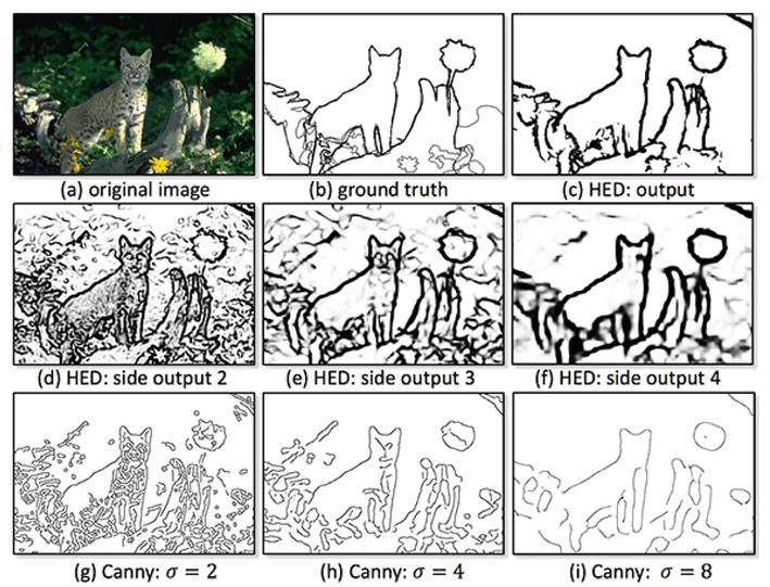
In Figure 7, we present a visual comparison between a recent algorithm (HED) and a traditional one (Canny). The HED represents deep learning algorithms well. It has gained a lot of success and has been integrated into the Opencv library. Canny, for its part, is the most recognized traditional algorithm, especially for its ability to cope with noise. From this figure, we can see the evolution of the HED output map through layers. We can see the performance limit of Canny algorithm, with three sigma parameter values. In terms of detection, HED presents very clear contours that are very close to the ground truth.

Figure 7.

Comparison of HED vs. Canny algorithms. (a) Image from the BSD500 dataset; (b) its corresponding annotated image; (c) the HED output. (d), (e), and (f), respectively, show side edge responses from layers 2, 3, and 4 of HED. (g), (h), and (i), show edge responses from the Canny detector respectively at the scales $\sigma$ = 2.0, $\sigma$ = 4.0, and $\sigma$ = 8.0.

6. Conclusions

Edge detection techniques have evolved significantly over the years, providing valuable tools for extracting important information from digital images. This chapter covered the basics of image edges, traditional edge detection algorithms, advanced techniques, challenges, and real-world applications. As technology continues to advance, especially in deep learning area, edge detection methods will continue to play a crucial role in various fields, paving the way for further research and innovation.

Despite these significant advancements, edge detection is still facing some challenges:

• Complexity: While network-based algorithms have significantly improved detection performance, they often come at the cost of increased computational complexity. In scenarios such as real-time video processing and embedded applications, the performance of these algorithms remains a limiting factor, preventing their full utilization.

• Variations in illumination conditions: Modern algorithms exhibit varying performance when applied to the same images under different lighting conditions, such as day and night. Such lack of performance underlines the challenges in achieving a consistent semantic understanding of image edges.

• Ambiguous edges: Some edges can be particularly challenging to interpret. For example, in the case of thick edges or in the case of zoomed images, some algorithms could predict these edges as two adjacent edges. This ambiguity underscores again the need for further refinement on semantic understanding of edges.

It is important to mention that the while presence of noise is a big challenge for traditional methods, supervised learning-based methods operates better in this case. This is related to the fact that these algorithms can be trained with augmented images with any kind of noise.

In light of these challenges, there is still ample room for research and improvement to enhance edge detection performance that affects other important applications that rely on edge detection such as image segmentation or object recognition.

Acknowledgments

This work was supported in part by the Imagin research team of Ecole Supérieur Privée d’Ingénierie et de Technologies. The authors would like to thank this research team for the valuable support and provided resources.

Conflict of interest

The authors declare no conflict of interest.

Abbreviations

CNN	convolutional neural network
ODS	optimal dataset scale
OIS	optimal image scale
ResNet	deep residual network
ROC	receiver operating characteristic
FOM	the figure of merit
SGD	stochastic gradient descent
ILSVRC	imagenet large scale visual recognition challenge competition

References

1.Ziou D, Tabbone S. Edge detection techniques - an overview. Pattern Recognition and Image Analysis C/C Raspoznavaniye Obrazov I Analiz Izobrazhenii. 1998;8:537-559
2.Shrivakshan GT, Chandrasekar C. A comparison of various edge detection techniques used in image processing. International Journal of Computer Science Issues (Ijcsi). 2012;9(5):269
3.Marr D, Hildreth E. Theory of edge detection. Proceedings of the Royal Society of London - Series B: Biological Sciences. 1980;207(1167):187-217. DOI: 10.1098/rspb.1980.0020
4.Sobel IE. Camera Models and Machine Perception [thesis]. Stanford: Stanford University; 1970
5.Xin Wang X. Laplacian operator-based edge detectors. IEEE Transactions on Pattern Analysis and Machine Intelligence. 2007;29(5):886-890. DOI: 10.1109/tpami.2007.1027
6.Canny J. A computational approach to edge detection. IEEE Transactions on Pattern Analysis and Machine Intelligence. 1986;PAMI-8:679-698. DOI: 10.1109/tpami.1986.4767851
7.Bertasius G, Shi J, Torresani L. Deepedge: A multi-scale bifurcated deep network for top-down contour detection. In: Proceedings of the IEEE Conference on Computer Vision and Pattern Recognition. Vol. 2015. Boston: IEEE; 2015a. pp. 4380-4389. DOI: 10.1109/cvpr.2015.7299067
8.Xie S, Tu Z. Holistically-nested edge detection. In: Proceedings of the IEEE International Conference on Computer Vision. Santiago: IEEE; 2015. pp. 1395-1403. DOI: 10.1109/iccv.2015.164
9.Deng R, Shen C, Liu S. Learning to predict crisp boundaries. In: Proceedings of the European Conference on Computer Vision (ECCV). Munich: Springer; 2018. pp. 562-578. DOI: 10.1007/978-3-030-01231-1-35
10.Simonyan K, Zisserman A. Very deep convolutional networks for large-scale image recognition. arXiv preprint. arXiv:1409.1556. 2014
11.Yang J, Price B, Cohen S. Object contour detection with a fully convolutional encoder-decoder network. In: Proceedings of the IEEE Conference on Computer Vision and Pattern Recognition. Las Vegas: IEEE; 2016. pp. 193-202. DOI: 10.1109/cvpr.2016.28
12.Su Z, Liu W, Yu Z. Pixel difference networks for efficient edge detection. arXiv preprint arXiv. 07009. 2021
13.Soria X, Sappa A, Humanante P, Akbarinia A. Dense extreme inception network for edge detection. Pattern Recognition. 2023;139:109461
14.Elharrouss O, Hmamouche Y, Idrissi AK, El Khamlichi B, El Fallah-Seghrouchni A. Refined edge detection with cascaded and high-resolution convolutional network. Pattern Recognition. 2023;138:109361
16.Krizhevsky A, Sutskever I, Hinton GE. Imagenet classification with deep convolutional neural networks. In: Advances in Neural Information Processing Systems 25. Vol. 25. San Francisco: Morgan Kaufmann Publishers Inc.; 2012. pp. 1097-1105
17.He K, Zhang X, Ren S. Deep residual learning for image recognition. In: Proceedings of the IEEE Conference on Computer Vision and Pattern Recognition. Las Vegas: IEEE; 2016. pp. 770-778. DOI: 10.1109/cvpr.2016.90
18.Yu Z, Feng C, Liu MY. Casenet: Deep category-aware semantic Edge Detection. In: Proceedings of the IEEE Conference on Computer Vision and Pattern Recognition. Honolulu: IEEE; 2017. pp. 5964-5973. DOI: 10.1109/cvpr.2017.191
19.Le T, Duan YE. REDN: A recursive encoder-decoder network for edge detection. IEEE Access. 2020;8:90153-90164. DOI: 10.1109/access.2020.2994160 Epub 2020 May 12
20.Pu M, Huang Y, Guan Q. RINDNet: Edge detection for discontinuity in reflectance. illumination, normal depth. arxiv Preprint arxiv. 00616. 2021
21.Kelm AP, Rao VS, Zolzer U. Object contour and edge detection with RefineContourNet. In: International Conference on Computer Analysis of Images and Patterns. Salerno: Springer; 2019. pp. 246-258. DOI: 10.1007/978-3-030-29888-3-20
22.Deng R, Liu S. Deep structural contour detection. In: Proceedings of the 28th ACM International Conference on Multimedia. New York: ACM; 2020. pp. 304-312
23.Martin DR, Fowlkes CC, Malik J. Learning to detect natural image boundaries using local brightness, color, and texture cues. IEEE Transactions on Pattern Analysis and Machine Intelligence. 2004;26:530-549
24.Bowyer K, Kranenburg C, Dougherty S. Edge detector evaluation using empirical ROC curves. Computer Vision and Image Understanding. 2001;84:77-103
25.Pratt WK, Wiley J. Digital Image Processing. New York: Citeseer; 1978
26.Arbelaez P, Maire M, Fowlkes C, Malik J. Contour detection and hierarchical image segmentation. IEEE Transactions on Pattern Analysis and Machine Intelligence. 2010;33:898-916
27.Berkeley Segmentation Dataset (BSDS500) download link. Available from: https://www2.eecs.berkeley.edu/Research/Projects/CS/vision/bsds/ [Accessed: September 01, 2023]
28.Silberman N, Hoiem D, Kohli P, Fergus R. Indoor segmentation and support inference from RGB-D images. In: European Conference on Computer Vision. Berlin: Springer; 2012. pp. 746-760
29.NYUD Datset download link. Available from: https://cs.nyu.edu/∼silberman/datasets/nyu_depth_v2.html [Accessed: September 01, 2023]
30.Everingham M, Eslami SA, Van Gool L, Williams CK, Winn J, Zisserman A. The pascal visual object classes challenge: A retrospective. International Journal of Computer Vision. 2015;111:98-136
31.Pascal-VOC dataset download link. Available from: http://host.robots.ox.ac.uk/pascal/VOC/voc2012/index.html [Accessed: September 01, 2023]
32.Mely DA, Kim J, McGill M, Guo Y, Serre T. A systematic comparison between visual cues for boundary detection. Vision Research. 2016;120:93-107
33.Multicue dataset download link. Available from: https://serre-lab.clps.brown.edu/resource/multicue/
34.Chollet F. Xception: Deep learning with Depthwise separable convolutions. In: Proceedings of the IEEE Conference on Computer Vision and Pattern Recognition. Las Vegas: IEEE; 2017. pp. 1251-1258. DOI: 10.1109/cvpr.2017.195
35.BIPED download link. Available from: https://xavysp.github.io/MBIPED/
36.Sun R, Lei T, Chen Q, Wang Z, Du X, Zhao W, et al. Survey of image edge detection. Frontiers in Signal Processing. 2022;2:826967
37.Jing J, Liu S, Wang G, Zhang W, Sun C. Recent advances on image edge detection: A comprehensive review. Neurocomputing. Vol. 503, No. C. 2022. pp. 259-271. DOI: 10.1016/j.neucom.2022.06.083
Written By
Anis BenHajyoussef and Asma Saidani
Submitted: 11 October 2023Reviewed: 17 October 2023Published: 15 January 2024