Perspective Chapter: Simulation and Analysis of Synthetic Aperture Radar Images

Abstract

The principal model for an image, generated by the interaction of an incident wave field with an inhomogeneous medium, is based on the ‘weak scattering approximation’. This approximation forms the basis for image processing, analysis and image understanding associated with applications over a broad range of frequencies. The physical limitations of such a model are typically overcome by introducing an additional stochastic field term that takes into account those effects that do not conform to the weak scattering approximation, coupled with background ‘system noise’. In this chapter, a solution to the scattering problem is presented, which is based on an exact scattering solution. An application of this solution is then considered which focuses on developing a model for a Synthetic Aperture Radar (SAR) image of the earth’s surface. By assuming that the surface is a fractal (a Mandelbrot surface), it is shown how an overhead optical image of the surface may be used to simulate a SAR image. The purpose of this is to generate training data for developing computer vision solutions using machine learning for autonomous navigation using SAR and for target detection in cases where only optical image data are available.

1. Introduction

Aperture synthesis is used in a wide range of applications including radar, sonar, diagnostic ultrasound and radio astronomy. The basic principle is very simple. In one form or another, the resolution of an image is determined by the size of the aperture that is used for observation. To improve the resolution, the size of the aperture must be increased. In some cases, to achieve a given resolution, an aperture must be used which is impractical either to build or utilise effectively. However, if a smaller aperture (a real aperture) is used, and its position changed while observations are being made, then, in effect, a much larger aperture can be synthesised.

Although the basic principles of aperture synthesis is the same, the details vary accord to the application. Radar (radio detection and ranging) has been used for many years (since the early 1940’s) to detect airborne objects using ground based antennas and to image the Earth’s surface using airbourne platforms.

Developments in the 1960s paved the way for a new generation of high resolution Radar systems which helped lead to the development of synthetic aperture radar (SAR) in the mid 1970s, although it had been used covertly for military and some space programmes well before that time (e.g. [1, 2]).

SAR was developed to study the surface of the Earth (and other planets) from both spacebourne and airborne platforms. Both systems attempt to classify the inhomogeneous nature of the Earth’s surface by repeatedly emitting a frequency modulated (chirped) pulse of microwave (GHz) radiation [3] and recording the back-scattered field. SAR systems essentially provide ‘microwave photographs’ of the Earth’s surface and are normally classified in terms of the wavelength that is used. Typical operational modes include X-band, with a wavelength of 2.8 cm, and L-band, with a wavelength of 24 cm. In addition to different wavelengths, different polarisations are used.

1.1 SAR imaging

A SAR image has a pixel resolution of the order of a metre or less, but the microwave scattering takes place on the scale of a centimetre. The return signals in range at each position of the moving real aperture are demodulated to base-band. Demodulation is coupled with quadrature detection, which provides the imaginary component of the real signal that is recorded, thereby generating the analytic signal [4].

The return (back-scattered) signals, which are generated by emitting a linear frequency modulated or chirped pulse of microwave radiation, are correlated with an identical chirp. This yields an Impulse Response Function (IRF) for the demodulated range signals given by a sinc function ($sinc\left(x\right)\equiv sin\left(x\right)/x$). However, the range at which the system operates is designed to exploit a model of the back-scattered microwave field that is in the Fresnel zone. Thus, the cross range (the direction at right angles to the range) response, is also a chirp function (both a down-chirp, in which the instantaneous frequency decreases, and an up-chirp, meaning that the instantaneous frequency increases). Hence, by correlating the combined return signals in cross range with the appropriate chirp function, the cross range data also becomes characterised by a sinc IRF. In this way, the two-dimensional (complex) data associated with a SAR image is classified by a point spread function (PSF) given by a separable sinc function. A grey scale image is then usually constructed by displaying the Amplitude Modulations associated with the processed data field.

1.2 Original contributions and structure

The principal focus of this work is concerned with the application of an exact scattering solution [5] and its implementation for modelling a SAR. In this respect, the material provide a ‘road map’ which starts with Maxwell’s equations for an Electromagnetic (EM) field and develops a solution that can be cast in terms of a standard model for a SAR image. This ‘standard’ involves the convolution of a characteristic Point Spread Function with an Object Function whose properties are determined by the scattering associated with the incidence of an EM wave field upon the ground surface.

The structure of the material is as follows: Section 2 provide a review of the EM field equations, casting them in a form that is suitable for generating a model for SAR. Section 3 introduces a scaler field model and the fundamental solution for the electric field. This is coupled with Section 4, which briefly discusses the differences between volume and surface scattering effects, followed by Section 5 which introduces the conventional weak scattering model. In this context, Sections 6 and 7 introduce the exact and strong scattering solutions, respectively; these sections are main components in regard to the most original themes of the material. Section 8 shows how the strong scattering solution can be used to develop a model for SAR and is followed with the introduction of another complementary idea which is concerns the use of a self-affine model for the scattering function. This is provided in Section 9, and is pivotal in the development of the approach presented in Section 10 which explores the basis for the numerical simulation of a SAR image using an optical image. The final components of the work are given in Sections 11 which investigate a vector field model, thereby introducing the effects of polarisation. It is shown how, a cross polarised field can be used to generate quantitative SAR images that differentiate between the dielectric and conductive properties of the ground surface. An Appendix is provided with a MATLAB function deigned to help readers appreciate the relative simplicity of the numerical simulations considered, to repeat the results presented, and provided the basis for further investigations and developments.

2. Electromagnetic field equations

Electromagnetic imaging systems require models to be constructed that are based on the field equations for electric and magnetic fields. These field equations are known as Maxwell’s equation, and in this section, we briefly introduce the macroscopic form of these equations for the case of an inhomogeneous conductive dielectric material. This provides a basis for the derivation of an inhomogeneous wave equation in regard to the electric field which forms the basis for the development of an EM imaging systems model.

For a linear, isotropic but inhomogeneous three-dimensional continuum with $\mathbf{r}\in {\mathrm{ℝ}}^3,r\equiv \mid \mathbf{r}\mid$, the macroscopic Maxwell’s equations are given by (for the International System of Units).

$$\nabla \cdot \epsilon \mathbf{E}=\rho$$E1

$$\nabla \cdot \mu \mathbf{H}=0$$E2

$$\nabla \times \mathbf{E}=-\mu \frac{\partial \mathbf{H}}{\partial t}$$E3

$$\nabla \times \mathbf{H}=\mathbf{J}+\epsilon \frac{\partial \mathbf{E}}{\partial t}$$E4

where $\mathbf{E}\left(\mathbf{r},t\right)$ is the electric field measured in Volts/metre, $\mathbf{H}\left(\mathbf{r},t\right)$ is the magnetic field in Amperes/metre, $\mathbf{J}\left(\mathbf{r},t\right)$ is the Current Density (Amperes/metre${}^2$), and $\rho \left(\mathbf{r},t\right)$ is the Charge Density (Coulombs/metre${}^3$). These fields are functions of space vector $\mathbf{r}$ and time $t$ and are related to the inhomogeneous (space varying) material parameters quantified by the electrical permittivity $\epsilon \left(\mathbf{r}\right)$ (Farads/metre) and the magnetic permeability $\mu \left(\mathbf{r}\right)$ (Henries/metre). Eqs. (1)–(4) represent (respectively) the differential forms of Coulombs law, the law of no magnetic monopoles, Faraday’s law of induction (electricity from magnetism) and Amperes law (magnetism from electricity) coupled with Maxwell’s additive displacement current term—the rate of change of an electric field.

The values of $\epsilon$ and $\mu$ in a vacuum (denoted by ${\epsilon }_0$ and ${\mu }_0$, respectively) are ${\epsilon }_0=8.854\times {10}^{-12}$ Farads/metre and ${\mu }_0=4\pi \times {10}^{-7}$ Henries/metre. In electromagnetic imaging problems there are two important physical models to consider, based on whether a material is conductive or non-conductive.

For a non-conductive material $\mathbf{J}=0$. In regard to a conductive material, the induced current depends on the magnitude of the electric field and the conductivity $\sigma$ (Siemens/metre) of the material. The relationship between the electric field and the current density is given by Ohm’s law which can be written in the form

$$\mathbf{J}=\sigma \mathbf{E}$$E5

Here, the current density is linearly related to the electric field alone, where for a good conductor, $\sigma >>1$. However, note that Eq. (5) is strictly only applicable to ‘Ohmic materials’ such as metals and some relatively poor conductors under specific circumstances. It is not applicable for semi-conductors, a moving Ohmic material in the presence of a magnetic field or for a plasma, for example, where, in the latter case, the generalised Ohm’s law for a plasma is required. Nevertheless, for the applications considered in this paper, Eq. (5) is sufficient for near-stationary conductive materials interacting with an EM field.

By taking the divergence of Eq. (4) and noting that

$$\nabla \cdot \left(\nabla \times \mathbf{H}\right)=0$$

then, given Eq. (1) for a constant $\epsilon$, and Eq. (5) for a constant $\sigma$, we can write

$$\frac{\partial \rho }{\partial t}+\frac{\sigma }{\epsilon }\rho =0\Rightarrow \rho \left(t\right)={\rho }_{0}exp\left(-\mathit{\sigma t}/\epsilon \right),{\rho }_0\equiv \rho \left(t=0\right)$$

This solution for the charge density shows that it decays exponentially with time. For typical values of $\epsilon \sim {10}^{-12}-{10}^{-10}$ Farads/metre, then, provided $\sigma$ is not too small, the dissipation of charge is very rapid. It is therefore physically reasonable to set the charge density to zero and, for problems involving the interaction of EM waves with good conductors, Eq. (1) can be approximated by

$$\nabla \cdot \epsilon \mathbf{E}=0$$E6

with Eq. (4) becoming

$$\nabla \times \mathbf{H}=\epsilon \frac{\partial \mathbf{E}}{\partial t}+\sigma \mathbf{E}$$

Note, that in EM imaging systems, the material may not necessarily be conductive throughout, but may be a varying dielectric with distributed conductive elements. For example, when imaging the Earth’s surface using microwave radiation, the EM scattering model can be based on a ‘ground truth’ that is predominantly a dielectric surface with localised conductors, e.g. metallic objects.

2.1 Wave equation

In electromagnetic imaging systems, a primary measurable field is the electric field, which induces a change in the voltage of the field detector. It is therefore appropriate to use a wave equation which describes the behaviour of the electric field. This can be obtained by decoupling Maxwell’s equations for the electric field $\mathbf{E}$. In regard to Eq. (3), dividing through by $\mu$ and taking the curl of the resulting equation yields

$$\nabla \times \left(\frac{1}{\mu }\nabla \times \mathbf{E}\right)=-\frac{\partial }{\partial t}\nabla \times \mathbf{H}.$$

By taking the derivative with respect to time of Eq. (4) and using Ohm’s law—Eq. (5)—we obtain

$$\frac{\partial }{\partial t}\left(\nabla \times \mathbf{H}\right)=\epsilon \frac{{\partial }^2\mathbf{E}}{\partial t^2}+\sigma \frac{\partial \mathbf{E}}{\partial t}.$$

From the previous equation we can then write

$$\nabla \times \left(\frac{1}{\mu }\nabla \times \mathbf{E}\right)=-\epsilon \frac{{\partial }^2\mathbf{E}}{\partial t^2}-\sigma \frac{\partial \mathbf{E}}{\partial t}$$E7

Expanding the first term, multiplying through by $\mu$ and noting that

$$\mu \nabla \left(\frac{1}{\mu }\right)=-\nabla ln\mu$$

we obtain

$$\nabla \times \nabla \times \mathbf{E}+\mathit{\epsilon \mu }\frac{{\partial }^2\mathbf{E}}{\partial t^2}+\mathit{\sigma \mu }\frac{\partial \mathbf{E}}{\partial t}=\left(\nabla ln\mu \right)\times \nabla \times \mathbf{E}$$

Further, expanding Eq. (6), we have

$$\epsilon \nabla \cdot \mathbf{E}+\mathbf{E}\cdot \nabla \epsilon =0\Rightarrow \nabla \cdot \mathbf{E}=-\mathbf{E}\cdot \nabla ln\epsilon$$

and hence, using the vector identity

$$\nabla \times \nabla \times \mathbf{E}=-{\nabla }^2\mathbf{E}+\nabla \left(\nabla \cdot \mathbf{E}\right)$$

we obtain the following wave equation for the electric field

$${\nabla }^2\mathbf{E}-\mathit{\epsilon \mu }\frac{{\partial }^2\mathbf{E}}{\partial t^2}-\mathit{\sigma \mu }\frac{\partial \mathbf{E}}{\partial t}=-\nabla \left(\mathbf{E}\cdot \nabla ln\epsilon \right)-\left(\nabla ln\mu \right)\times \nabla \times \mathbf{E}$$E8

This equation is inhomogeneous in $\epsilon$, $\mu$ and $\sigma$. Solutions to this equation provide information on the behaviour of the electric field in an inhomogeneous conductive dielectric environment. In electromagnetic imaging problems, interest focuses on the behaviour of the scattered EM field generated by variations in the material parameters $\epsilon$, $\mu$ and $\sigma$. The problem is to reconstruct, or to at least interpret these parameters by measuring certain properties of the scattered electric field. This is a three parameter inverse problem which requires us to solve for the electric field $\mathbf{E}$ given $\epsilon ,\mu$ and $\sigma$. In the context of the model considered, a similar type of analysis can be implemented to generate an inhomogeneous wave equation for the magnetic field which is given by

$${\nabla }^2\mathbf{H}-\mathit{\epsilon \mu }\frac{{\partial }^2\mathbf{H}}{\partial t^2}-\mathit{\sigma \mu }\frac{\partial \mathbf{H}}{\partial t}=-\nabla \left(\mathbf{H}\cdot \nabla ln\mu \right)-\left(\nabla ln\epsilon \right)\times \nabla \times \mathbf{H}-\epsilon \mathbf{E}\times \nabla \left(\frac{\sigma }{\epsilon }\right)$$

Note, that in this case, the equation for $\mathbf{H}$ is coupled to $\mathbf{E}$ through the last term on the right hand side. It is for this reason that the wave equation for the electric field given by Eq. (8) is considered. Moreover, Eq. (8) is consistent with the development of a ‘systems model’ where the imaging data is based on the detection of the electric wave field; this includes Real and Synthetic Aperture Radar’s.

2.2 Inhomogeneous wave equation

In order to solve the wave equation (focusing on the electric field) derived in the last section using the most appropriate analytical methods for imaging science (i.e. the fundamental Green function solution, as discussed later), it is typically re-cast in the form of the (time-independent) Langevin equation

$$\left({\nabla }^2+k^2\right)\mathbf{E}=-\widehat{L}\mathbf{E}$$

where $\widehat{L}$ is an inhomogeneous differential operator, $\left({\nabla }^2+k^2\right)$ is the Helmholtz operator, and $k=2\pi /\lambda$ is the wavenumber associated with the wavelength $\lambda$.

To achieved this, we first modify the time dependent equation, starting by adding the term

$${\epsilon }_0\frac{{\partial }^2\mathbf{E}}{\partial t^2}-\frac{1}{{\mu }_0}\nabla \times \nabla \times \mathbf{E}$$

to both sides of Eq. (7), so that, upon re-arranging, we can write

$$\nabla \times \nabla \times \mathbf{E}+{\epsilon }_0{\mu }_0\frac{{\partial }^2\mathbf{E}}{\partial t^2}=-{\epsilon }_0{\mu }_0{\gamma }_{\epsilon }\frac{{\partial }^2\mathbf{E}}{\partial t^2}-{\mu }_0\sigma \frac{\partial \mathbf{E}}{\partial t}+\nabla \times \left({\gamma }_{\mu }\nabla \times \mathbf{E}\right)$$E9

where

$${\gamma }_{\epsilon }=\frac{\epsilon -{\epsilon }_0}{{\epsilon }_0}={\epsilon }_r-1\text{and}{\gamma }_{\mu }=\frac{\mu -{\mu }_0}{\mu }=1-\frac{1}{{\mu }_r}$$

Here, ${\epsilon }_r\ge 1$ and ${\mu }_r\ge 1$ are dimensionless variables—the relative permittivity and the relative permeability, respectively. We can then use the result (which is valid for $\rho \sim 0$ in Eq. (1), when $\sigma >>1$)

$$\nabla \times \nabla \times \mathbf{E}=-{\nabla }^2\mathbf{E}+\nabla \left(\nabla \cdot \mathbf{E}\right)=-{\nabla }^2\mathbf{E}-\nabla \left(\mathbf{E}\cdot \nabla ln\epsilon \right)$$

so that Eq. (9) can now be written as

$${\nabla }^2\mathbf{E}-{\epsilon }_0{\mu }_0\frac{{\partial }^2\mathbf{E}}{\partial t^2}={\mu }_0{\epsilon }_0{\gamma }_{\epsilon }\frac{{\partial }^2\mathbf{E}}{\partial t^2}+{\mu }_0\sigma \frac{\partial \mathbf{E}}{\partial t}-\nabla \left(\mathbf{E}\cdot \nabla ln\epsilon \right)-\nabla \times \left({\gamma }_{\mu }\nabla \times \mathbf{E}\right)$$E10

2.3 Time independent wave equation

Construction of a time-independent wave equation can be undertaken by considering the time dependence of the electric field to be harmonic when $\mathbf{E}\left(\mathbf{r},t\right)\equiv \mathbf{E}\left(\mathbf{r},\omega \right)exp\left(\mathit{i\omega t}\right)$ where $\omega$ is a constant angular frequency, thereby allowing Eq. (10) to be cast in the form of the following inhomogeneous Helmholtz equation [6] for a vector field:

$$\left({\nabla }^2+k^2\right)\mathbf{E}=-k^2{\gamma }_{\epsilon }\mathbf{E}+{\mathit{ikZ}}_0\sigma \mathbf{E}-\nabla \left(\mathbf{E}\cdot \nabla ln\epsilon \right)-\nabla \times \left({\gamma }_{\mu }\nabla \times \mathbf{E}\right)$$E11

where

$$k=2\mathit{\pi \lambda }=\omega c_0,c_0=\frac{1}{\sqrt{{\epsilon }_0{\mu }_0}}\text{and}{Z}_0={\mu }_0{c}_0.$$

The parameter $Z_0$ is the free space wave impedance and is approximately equal to $377$ Ohms. The constant $c_0$ is the velocity at which EM waves propagate in a perfect vacuum—the speed of light$\simeq 3\times {10}^8{\mathrm{ms}}^{-1}$. In electromagnetic imaging, images are characterised by the spatial variations of the parameters ${\gamma }_{\epsilon }$, ${\gamma }_{\mu }$ and the conductivity $\sigma$.

Eq. (11) also applies to the case when the time-dependence of the electric field can be described in terms of a spectrum of frequencies when $\mathbf{E}\left(\mathbf{r},t\right)$ is related to the temporal frequency spectrum $\mathbf{E}\left(\mathbf{r},\omega \right)$ through the Fourier transform, i.e.

$$\mathbf{E}\left(\mathbf{r},t\right)\leftrightarrow \mathbf{E}\left(\mathbf{r},\omega \right),\mathbf{E}\left(\mathbf{r},t\right)=\frac{1}{2\pi }\underset{-\infty }{\overset{\infty }{\int }}\mathbf{E}\left(\mathbf{r},\omega \right)exp\left(\mathit{i\omega t}\right)\mathit{d\omega }$$

where $\leftrightarrow$ denotes the Fourier transform pair.

Eq. (11) is the wave field model upon which all of the material that follows in this article is based. This material is concerned with two distinct models for a Synthetic Aperture Radar system in association with Eq. (11). The first is a scalar field model when the last two terms on the right hand side of Eq. (11) are neglected. The second model considers a solution to Eq. (11) based on neglecting the last term on the right hand side which is consistent with imposing the condition that ${\mu }_r=1$.

3. Scalar field model

In regard to Eq. (11), a scalar wave field model is compounded in the equation

$$\left({\nabla }^2+k^2\right)E\left(\mathbf{r},k\right)=\gamma \left(\mathbf{r},k\right)E\left(\mathbf{r},k\right)$$E12

where

$$\gamma \left(\mathbf{r},k\right)=-k^2{\gamma }_{\epsilon }\left(\mathbf{r}\right)+{\mathit{ikZ}}_0\sigma \left(\mathbf{r}\right)$$E13

The field $E\left(\mathbf{r},k\right)$ denotes any component of the electric field vector $\mathbf{E}\left(\mathbf{r},k\right)=\widehat{\mathbf{x}}{E}_x\left(\mathbf{r},k\right)+\widehat{\mathbf{y}}{E}_y\left(\mathbf{r},k\right)+\widehat{\mathbf{z}}{E}_z\left(\mathbf{r},k\right)$ where ($\widehat{\mathbf{x}},\widehat{\mathbf{y}},\widehat{\mathbf{z}}$) are unit vectors in a Euclidean space and $(E_x,E_y,E_z$) are the scalar components of the field in that space.

This equation has the fundamental Green’s function solution [7].

$$E\left(\mathbf{r},k\right)=E_i\left(\mathbf{r},k\right)+E_s\left(\mathbf{r},k\right)$$E14

where $E_i\left(\mathbf{r},k\right)$ is the incident wave function, taken to be a solution of the homogenous Helmholtz equation

$$\left({\nabla }^2+k^2\right)E_i\left(\mathbf{r},k\right)=0$$E15

and $E_s\left(\mathbf{r},k\right)$ is the scattered field given by

$$E_s\left(\mathbf{r},k\right)=g\left(r,k\right){\otimes }_{\mathbf{r}}\gamma \left(\mathbf{r},k\right)E\left(\mathbf{r},k\right)\text{where}g\left(r,k\right)=\frac{exp\left(\mathit{ikr}\right)}{4\mathit{\pi r}}$$E16

The function $g\left(r,k\right)$ is the ‘out-going free-space Green’s function’ which is the solution of [7].

$$\left({\nabla }^2+k^2\right)g\left(r,k\right)={\delta }^3\left(\mathbf{r}\right)$$E17

for the three-dimensional delta function ${\delta }^3\left(\mathbf{r}\right)$ and the operator ${\otimes }_{\mathbf{r}}$ denotes the convolution integral, i.e.

$$g\left(\mathbf{r}\right){\otimes }_{\mathbf{r}}f\left(\mathbf{r}\right)\equiv \underset{-\infty }{\overset{\infty }{\int }}g\left(\mathbf{r}-\mathbf{s}\right)f\left(\mathbf{s}\right)d^n\mathbf{s}$$

where $\left[g\left(\mathbf{r}\right),f\left(\mathbf{r}\right)\right]\in L^2\left({\mathrm{ℝ}}^3\right):\mathrm{ℂ}\to \mathrm{ℂ}$. Thus, we note that

$$g\left(r,k\right){\otimes }_{\mathbf{r}}\gamma \left(\mathbf{r},k\right)E\left(\mathbf{r},k\right)\equiv \underset{-\infty }{\overset{\infty }{\int }}g\left(\mathbf{r}|\mathbf{s},k\right)\gamma \left(\mathbf{s},k\right)E\left(\mathbf{s},k\right)d^3\mathbf{s}$$

where, for notational convenience and clarity, $g\left(\mathbf{r}|\mathbf{s},k\right)\equiv g\left(|\mathbf{r}-\mathbf{s}|,k\right)$.

A simple proof of the fundamental solution given by Eq. (16) is obtained by noting that

$$\begin{array}{ll}{\nabla }^{2}E\left(\mathbf{r},k\right)& ={\nabla }^2{E}_i\left(\mathbf{r},k\right)+{\nabla }^2\left[g\left(r,k\right){\otimes }_{\mathbf{r}}\gamma \left(\mathbf{r},k\right)E\left(\mathbf{r},k\right)\right]\\ & ={\nabla }^2{E}_i\left(\mathbf{r},k\right)+{\nabla }^2\left[g\left(r,k\right)\right]{\otimes }_{\mathbf{r}}\gamma \left(\mathbf{r},k\right)E\left(\mathbf{r},k\right)\\ & ={\nabla }^2{E}_i\left(\mathbf{r},k\right)+\left[{\delta }^3\left(\mathbf{r}\right)-k^{2}g\left(r,k\right)\right]{\otimes }_{\mathbf{r}}\gamma \left(\mathbf{r},k\right)E\left(\mathbf{r},k\right)\\ & ={\nabla }^2{E}_i\left(\mathbf{r},k\right)+\gamma \left(\mathbf{r},k\right)E\left(\mathbf{r},k\right)-k^2\left[E\left(\mathbf{r},k\right)-E_i\left(\mathbf{r},k\right)\right]\\ & =-k^{2}E\left(\mathbf{r},k\right)+\gamma \left(\mathbf{r},k\right)E\left(\mathbf{r},k\right)\end{array}$$E18

given Eqs. (15) and (17), and that

$${\delta }^3\left(r\right){\otimes }_{\mathbf{r}}\gamma \left(\mathbf{r},k\right)E\left(\mathbf{r},k\right)=\gamma \left(\mathbf{r},k\right)E\left(\mathbf{r},k\right)$$

In the context of Eq. (16), the forward scattering problem is ‘Given $\gamma \left(\mathbf{r},k\right)$ evaluate $E_s\left(\mathbf{r},k\right)$’. The corresponding inverse scattering problem is ‘Given $E_s\left(\mathbf{r},k\right)$ evaluate $\gamma \left(\mathbf{r},k\right)$’. Both problems ideally require unconditional and exact solutions. If the ‘scattering function’ $\gamma \left(\mathbf{r},k\right)$ is taken to be a piecewise continuous function over all space, approaching zero at infinity say, then there are no boundary conditions that need to be taken into account. However, Eq. (14) also applies to the case of a scattering function of compact support with a defined surface for which boundary conditions apply. This is discussed in the following section.

4. Volume and surface scattering effects

Eq. (14) is valid for for $\gamma \left(\mathbf{r},k\right)\to 0\mathrm{as}r\to \infty$. In the case when $\gamma \left(\mathbf{r},k\right)$ is a function of compact support such that $\mathbf{r}\in V$ where $V$ is a finite volume of space, the fundamental solution is [7].

$$E\left(\mathbf{r},k\right)=\underset{\mathbf{s}\in V}{\int }g\left(\mathbf{r}|\mathbf{s}\right)\gamma \left(\mathbf{s},k\right)E\left(\mathbf{s},k\right)d^3\mathbf{s}+\underset{\mathbf{s}\in S}{\oint }\left[g\left(\mathbf{r}|\mathbf{s}.k\right)\nabla E\left(\mathbf{s},k\right)-E\left(\mathbf{s},k\right)\nabla g\left(\mathbf{r}|\mathbf{s},k\right)\right]\cdot \widehat{\mathbf{n}}{d}^2\mathbf{s}$$

where $S$ defines the surface of the scattering function and $\widehat{\mathbf{n}}$ is the outward unit normal at each point on $S$.

If the field does not penetrate into the volume of the scatterer, then the solution is given by the surface integral alone. The solution then depends explicitly on the values of the field (and its gradient) on the boundary of the surface alone, from which the surface integral may then be evaluated. This is a boundary value problem whose solutions describe surface scattering effects and applies to scattering problems when there is no propagation of the incident field into the interior of the scatterer.

When the incident field penetrates into the interior of the scatterer, both volume and surface scattering effects must be taken into account. This is the case when the scatterer is composed on (non-conductive) dielectric materials, for example. Thus, suppose that the field $E_i\left(\mathbf{r},k\right)$, which is a solution to Eq. (15), is incident upon the surface of the scatterer. At the point of incidence, the boundary field and its gradient will be $E_i\left(\mathbf{s},k\right)$ and $\nabla E_i\left(\mathbf{s},k\right)$, respectively. Using these boundary conditions and Green’s theorem [7], we have

$$\begin{array}{c}\underset{\mathbf{s}\in S}{\oint }\left[g\left(\mathbf{r}|\mathbf{s},k\right)\nabla E_i\left(\mathbf{s},k\right)-E_i\left(\mathbf{s},k\right)\nabla g\left(\mathbf{r}|\mathbf{s},k\right)\right]\cdot \widehat{\mathbf{n}}{d}^2\mathbf{s}\\ =\underset{\mathbf{s}\in V}{\int }\left[g\left(\mathbf{r}|\mathbf{s},k\right){\nabla }^2{E}_i\left(\mathbf{s},k\right)-E_i\left(\mathbf{s},k\right){\nabla }^{2}g\left(\mathbf{r}|\mathbf{s},k\right)\right]d^3\mathbf{s}=\underset{\mathbf{s}\in V}{\int }{\delta }^3\left(\mathbf{r}-\mathbf{s}\right)E_i\left(\mathbf{s},k\right)d^3\mathbf{s}=E_i\left(\mathbf{r},k\right)\end{array}$$

having noted that

$${\nabla }^2{E}_i\left(\mathbf{r},k\right)=-k^2{E}_i\left(\mathbf{r},k\right)\text{and}{\nabla }^{2}g\left(\mathbf{r}|\mathbf{s},k\right)=-{\delta }^3\left(\mathbf{r}-\mathbf{s}\right)-k^{2}g\left(\mathbf{r}|\mathbf{s},k\right)$$

Hence, we obtain the same solution as given by Eq. (14) for a scattering function of compact support (or otherwise) with a defined surface upon which the electric field and its gradient are taken to be that of an incident field conforming to Eq. (15). It may be argued that this is also valid for conductive scatterers unless the skin depth, given by $\delta ={\left(2/{\mathit{kZ}}_0\sigma \right)}^{1/2}$, is taken to be zero (implying that the conductivity is infinite!). In practice, however, the skin depth is finite and thus, Eq. (14) may be applied for a volume that is determined by the surface and the skin depth of the scatterer where, beyond the skin depth, the field is taken to be zero. In this way, a volume scattering model can be applied for cases involving field attenuating scatterers such conductors where $\sigma >>0$.

5. Weak scattering model: The born approximation

Eq. (14) is an integral equation obtained through application of the fundamental Green’s function solution. However, it is not a solution. This is because the $E\left(\mathbf{r},k\right)$ field is on both the left and right hand sides of the equation. The simplest, and most common solution to this problem, is obtained by applying what is commonly referred to as the Born approximation [8]. This is where it is assumed that the convolution integral for the scattered field can be approximated using the result

$$E_s\left(\mathbf{r},k\right)=g\left(r,k\right){\otimes }_{\mathbf{r}}\gamma \left(\mathbf{r},k\right)E_i\left(\mathbf{r},k\right)$$E19

Application of this approximation requires that

$$\frac{\parallel E_s\left(\mathbf{r},k\right){\parallel }_2}{\parallel E_i\left(\mathbf{r},k\right){\parallel }_2}<<1$$E20

where $\parallel •{\parallel }_2$ denotes the Euclidean norm. Essentially, Condition (20) means that the intensity of the field $E_s\left(\mathbf{r},k\right)$ (the scattering cross-section) is small compared to that of $E_i\left(\mathbf{r},k\right)$. The condition implies that the scattering is a ‘weak effect’, i.e., the scattered field is a small perturbation of the incident field. In physical terms, this means that there are no multiple scattering effects taken to be present. Thus, the Born scattered field is a model for single scattering events alone.

Multiple scattering events can be taken into account through iteration of Eq. (14) which requires that the series converges. This is a formal solution to the (multiple) scattering problem, and is quantified in terms of the series solution to Eq. (14), given by

$$E\left(\mathbf{r},k\right)=E_i\left(\mathbf{r},k\right)+g\left(r,k\right){\otimes }_{\mathbf{r}}\gamma \left(\mathbf{r},k\right)E_i\left(\mathbf{r},k\right)+g\left(r,k\right){\otimes }_{\mathbf{r}}\gamma \left(\mathbf{r},k\right)\left[g\left(r,k\right){\otimes }_{\mathbf{r}}\gamma \left(\mathbf{r},k\right)E_i\left(\mathbf{r},k\right)\right]+\dots$$

The Born approximation is then observed to be the first iteration of a series solution, each higher order term of the series representing the second, third, fourth etc. order scattering effects. In this context, we can analyse the physical limitations that the Born approximation exhibits. To do this, Condition (20) must be investigated further.

The Born approximation requires that $E_s\left(\mathbf{r},k\right)$ is ‘small’ compared to $E_i\left(\mathbf{r},k\right)$ for all $\mathbf{r}\in {\mathrm{ℝ}}^3$ and $k$. To quantify this statement, we use Young’s convolution inequality and then Hölder’s inequality, respectively. For a Euclidean, this yields the result:

$$\begin{array}{ll}\parallel E_s\left(\mathbf{r},k\right){\parallel }_2& =\parallel g\left(\mathbf{r},k\right){\otimes }_{\mathbf{r}}\gamma \left(\mathbf{r},k\right)E_i\left(\mathbf{r},k\right){\parallel }_2\le \parallel g\left(\mathbf{r},k\right){\parallel }_2\parallel \gamma \left(\mathbf{r},k\right)E_i\left(\mathbf{r},k\right){\parallel }_2\\ & \le \parallel E_i\left(\mathbf{r},k\right){\parallel }_2\parallel g\left(\mathbf{r},k\right){\parallel }_2\parallel \gamma \left(\mathbf{r},k\right){\parallel }_2\end{array}$$

It is then clear that the condition for the Born approximation to hold can be written as

$$\parallel g\left(\mathbf{r},k\right){\parallel }_2\parallel \gamma \left(\mathbf{r},k\right){\parallel }_2<<1$$

For a scatterer that is taken to be a sphere of radius $R$ say, we can write the condition as

$$⟨\gamma \left(\mathbf{r},k\right)⟩<<1R^2\text{where}⟨\gamma \left(\mathbf{r},k\right)⟩\equiv \sqrt{\frac{\int {\left|\gamma \left(\mathbf{r},k\right)\right|}^2{d}^3\mathbf{r}}{\int d^3\mathbf{r}}}$$

Thus, for a dielectric material when $\gamma \left(\mathbf{r},k\right)=-k^2{\gamma }_{\epsilon }\left(\mathbf{r}\right)$ (and $\sigma =0$), we can write the condition in terms of the wavelength $\lambda$ as

$$\lambda >>R\sqrt{⟨\gamma \left(\mathbf{r},k\right)⟩}$$

This ‘distillation’ of the condition for the Born approximation to be applicable, demonstrates that, for arbitrary values of $⟨\gamma \left(\mathbf{r},k\right)⟩$, Condition (20) holds, provided the physical scale length $L$ say, of the scattering function is small compared to the wavelength. Else, for scale lengths where $L\sim \lambda$, the condition for the Born approximation to apply is $⟨\gamma \left(\mathbf{r},k\right)⟩<<1$. This is the condition required for the scatterer to be classified as being ‘weak’.

The main point here, is that unless the scattering is taken to be weak, the Born approximation can only be satisfied if $\lambda >>L$. However, this condition is entirely incompatible with a fundamental reality concerning the structural information associated with any and all images formed from a scattering interaction. This is that information on the structure of a material is determined by the interactions that take place on the scale of a wavelength. It is this dichotomy, at least, for scattering effects that cannot be classified as being ‘weak’ which is the more common physical reality, that lies at the heart of the problem in using a Born scattering model to processes and analyse images obtained from the scattering of an EM field. For this reason, the approach considered in the following section is now presented.

6. Exact scattering model

For a scalar field, an exact scattering solution to Eq. (12) can be formulated which is compounded in the result [5].

$$E\left(\mathbf{r},k\right)=g\left(r,k\right){\otimes }_{\mathbf{r}}\gamma \left(\mathbf{r},k\right)E_i\left(\mathbf{r},k\right)$$E21

where, for spatial frequency vector $\mathbf{u}$,

$$\begin{array}{c}E\left(\mathbf{r},k\right)\leftrightarrow \frac{{\tilde{E}}_i\left(\mathbf{u},k\right){\tilde{E}}_s\left(\mathbf{u},k\right)}{{\tilde{E}}_i\left(\mathbf{u},k\right)+{\tilde{E}}_s\left(\mathbf{u},k\right)},\\ {\tilde{E}}_i\left(\mathbf{u},k\right)\leftrightarrow E_i\left(\mathbf{r},k\right),{\tilde{E}}_s\left(\mathbf{u},k\right)\leftrightarrow E_s\left(\mathbf{r},k\right)\text{and}\tilde{E}\left(\mathbf{u},k\right)=\underset{-\infty }{\overset{\infty }{\int }}E\left(\mathbf{r},k\right)exp\left(-i\mathbf{u}\cdot \mathbf{r}\right)d^3\mathbf{r}\end{array}$$E22

Equation (21) facilitates an exact (near-field) inverse scattering solution given that we can write

$$\gamma \left(\mathbf{r},k\right)=\frac{E_i^{\ast }\left(\mathbf{r},k\right)}{{\left|E_i\left(\mathbf{r},k\right)\right|}^2}h\left(r,k\right){\otimes }_{\mathbf{r}}E\left(\mathbf{r},k\right)\text{where}h\left(r,k\right){\otimes }_{\mathbf{r}}g\left(r,k\right)={\delta }^3\left(\mathbf{r}\right)$$

However, Eq. (21) is subject to Eq. (15), and, more critically, a further ‘conditioning equation’ given by [5].

$$\left({\nabla }^2+k^2\right)\gamma \left(\mathbf{r},k\right)E_i\left(\mathbf{r},k\right)=0$$E23

This is a non-standard condition that requires quantification in terms of the class of scattering functions that are applicable. In this respect, expanding Eq. (23), we can write it in the form

$${\nabla }^2\gamma \left(\mathbf{r},k\right)+2\nabla \gamma \left(\mathbf{r},k\right)\cdot \nabla ln{E}_i\left(\mathbf{r},k\right)=0$$

and thus, for an incident unit plane wave field given by $E_i\left(\mathbf{r},k\right)=exp\left(-i\mathbf{k}\cdot \mathbf{r},/,2\right)$ say, which is a solution to Eq. (15), we can write Eq. (23) as

$${\nabla }^2\gamma \left(\mathbf{r},k\right)-i\mathbf{k}\cdot \nabla \gamma \left(\mathbf{r},k\right)=0$$E24

Eq. (24) has a solution (for arbitrary constants $a$ and $b$) given by

$$\gamma \left(\mathbf{r},k\right)=a+bexp\left(i\mathbf{k}\cdot \mathbf{r}\right)$$

However under the condition that $\mathbf{k}\cdot \mathbf{u}-u^2=0$, Eq. (24) has the general solution

$$\gamma \left(\mathbf{r},k\right)=\frac{1}{{\left(2\pi \right)}^3}\underset{-\infty }{\overset{\infty }{\int }}\tilde{\gamma }\left(\mathbf{u},k\right)exp\left(i\mathbf{u}\cdot \mathbf{r}\right)d^3\mathbf{u}$$

Therefore, Eq. (23) allows Eq. (21) to hold for any scattering function for which a definable frequency spectrum $\tilde{\gamma }\left(\mathbf{u},k\right)$ exists, subject to the condition $u\equiv \mid \mathbf{u}\mid =kcos\theta$. An interpretation of this condition can be formulated for the case when $\theta \sim 0$ (i.e. $\mathbf{u}\sim \mathbf{k}$) or $k/u\sim 1$ as follows: Suppose that the temporal frequency is a constant $k_0$ where $k_0>>1$. Further, let the spatial frequency spectrum of $\gamma \left(\mathbf{r},k_0\right)$, over which spectral information is attainable, have a bandwidth $K$, such that (for the positive frequency half space) $u\in \left[k_0\pm K\right]$ where $K/k_0<<1$. Then, $k_0/u\sim 1$. This condition is compatible with the use of a narrow side-band imaging system such as a SAR, and, in this respect, the exact scattering solution is applicable for modelling such a system. This analysis applies to the case when $E_i\left(\mathbf{r},k\right)=P\left(k\right)exp\left(\pm i\mathbf{k}\cdot \mathbf{r}\right)$ for any amplitude spectrum $P\left(k\right)$. In this context, given Eq. (23), we can write Eq. (21) as

$$E\left(\mathbf{r},k\right)=-1k^{2}g\left(r,k\right){\otimes }_{\mathbf{r}}{\nabla }^2\left[\gamma \left(\mathbf{r},k\right)E_i\left(\mathbf{r},k\right)\right]$$E25

where $k\sim k_0>>1$.

In terms of Eq. (21), it is noted that, subject to the condition,

$$\parallel {\tilde{E}}_s\left(\mathbf{u},k\right){\parallel }_2<<\parallel {\tilde{E}}_i\left(\mathbf{u},k\right){\parallel }_2$$E26

then

$$\frac{{\tilde{E}}_i\left(\mathbf{u},k\right){\tilde{E}}_s\left(\mathbf{u},k\right)}{{\tilde{E}}_i\left(\mathbf{u},k\right)+{\tilde{E}}_s\left(\mathbf{u},k\right)}=\frac{{\tilde{E}}_s\left(\mathbf{u},k\right)}{1+{\tilde{E}}_s\left(\mathbf{u},k\right)/{\tilde{E}}_i\left(\mathbf{u},k\right)}\simeq {\tilde{E}}_s\left(\mathbf{u},k\right)$$

In this case, we may consider the approximate relationship

$$E\left(\mathbf{r},k\right)\leftrightarrow {\tilde{E}}_s\left(\mathbf{u},k\right)$$

and Eq. (21) reduces to

$$E_s\left(\mathbf{r},k\right)=g\left(r,k\right){\otimes }_{\mathbf{r}}\gamma \left(\mathbf{r},k\right)E_i\left(\mathbf{r},k\right)$$E27

This result is equivalent to the Born approximation discussed in Section 5. The exact scattering solution given by Eq. (21) [subject to the condition compounded in Eq. (23)] therefore reduces to the Born approximation under the condition that the spectrum of the scattered field is weaker than the spectrum of the incident field. Note, that Condition (26) is equivalent to Condition (20), given Rayleigh’s energy theorem, i.e.

$$\parallel E\left(\mathbf{r},k\right){\parallel }_2^2=\frac{1}{{\left(2\pi \right)}^3}\parallel \tilde{E}\left(\mathbf{u},k\right){\parallel }_2^2$$

7. Strong scattering model

While Eq. (21) provides an exact scattering solution, subject to Condition (23), it does not provide an expression for the scattered field itself. To achieve this, we consider the following approach: Using a binomial expansion, the scattered field spectrum can be written as

$$\begin{array}{l}{\tilde{E}}_s\left(\mathbf{u},k\right)=\frac{{\tilde{E}}_i\left(\mathbf{u},k\right)\tilde{E}\left(\mathbf{u},k\right)}{{\tilde{E}}_i\left(\mathbf{u},k\right)-\tilde{E}\left(\mathbf{u},k\right)}=\tilde{E}\left(\mathbf{u},k\right)\left(1+\frac{\tilde{E}\left(\mathbf{u},k\right)}{{\tilde{E}}_i\left(\mathbf{u},k\right)}+\dots \right),\left|\frac{\tilde{E}\left(\mathbf{u},k\right)}{{\tilde{E}}_i\left(\mathbf{u},k\right)}\right|<1\\ \end{array}$$

Given Eq. (25), we observe that the $n^{\mathrm{th}}$ term of this binomial series scales as $k^{-2n}$, and for this reason, we can write

$${\tilde{E}}_s\left(\mathbf{u},k\right)=\tilde{E}\left(\mathbf{u},k\right),\mid k\mid \to \infty$$

Thus, we obtain an expression for a high frequency scattered field, given by

$$E_s\left(\mathbf{r},k\right)=-\frac{1}{k^2}g\left(r,k\right){\otimes }_{\mathbf{r}}{\nabla }^2\left[\gamma \left(\mathbf{r},k\right)E_i\left(\mathbf{r},k\right)\right],\mid k\mid >>1$$E28

Apart from a scaling factor by $k^{-2}$, the major difference between the weak scattering solution given by Eq. (27) and Eq. (28) is compounded in the Laplacian operator ${\nabla }^2$. In this context, the scattered field given by Eq. (28) is referred to as a ‘strong scattering solution’.

Unlike the Born approximation, this solution is exact and subject only to Eq. (23) for $\mid k\mid >>1$. The high frequency condition means that Eq. (28) is not suitable for base-band imaging systems where $k\in \left[-K,K\right]$ for bandwidth $K$. However, it is appropriate for sideband systems where (for the positive frequency half-space) $k\in \left[k_0\pm K\right]$ when $k_0>>1$ and $K/k_0<<1$.

A further modification to Eq. (28) can be made by noting that, for a unit plane wave, when $E_i\left(\mathbf{r},k\right)=exp\left(i\mathbf{k}\cdot \mathbf{r}\right)$ say, which is a solution to Eq. (15), then

$$\begin{array}{ll}{\nabla }^2\left[\gamma \left(\mathbf{r},k\right)E_i\left(\mathbf{r},k\right)\right]& =exp\left(i\mathbf{k}\cdot \mathbf{r}\right)\left[{\nabla }^2\gamma \left(\mathbf{r},k\right)+2i\mathbf{k}\cdot \nabla \gamma \left(\mathbf{r},k\right)-k^2\gamma \left(\mathbf{r}\right)\right]\\ & \sim exp\left(i\mathbf{k}\cdot \mathbf{r}\right){\nabla }^2\gamma \left(\mathbf{r},k\right)\end{array}$$E29

This result is based on a further condition which is that the second order gradient of the scattering function dominates (in amplitude) the first order gradient and the scattering function itself, given that the wavelength is taken to be relatively large compared to the scale length over which a gradient occurs. Note, that this is not the same as applying the Born approximation, which is predicated on the wavelength being large compared to the scale length of the scatterer itself (and not its first and second order gradients).

8. Model for a SAR image

As briefly discussed in the introduction, a SAR is based on repeatedly emitting a frequency modulated pulse in range as the radar platform moves cross range, usually at a fixed height. The pulse forms part of an emitted beam that, in regard to the scattering events that take place, has a range that is ‘engineered’ to be in the Fresnel zone. Thus, the Green’s function given in Eq. (28) must be modified to reflect this reality. In terms of the convolution integral given in Eq. (28), and, with a slight change of notation, we consider the following expression for the Green’s function as a convolution kernel:

$$g\left(\mathbf{r}|{\mathbf{r}}_0,k\right)\equiv \frac{1}{4\pi \mid \mathbf{r}-{\mathbf{r}}_0\mid }exp\left(\mathit{ik}|\mathbf{r}-{\mathbf{r}}_0|\right),\mathbf{r}\mid {\mathbf{r}}_0\equiv \mid \mathbf{r}-{\mathbf{r}}_0\mid$$

For a SAR, the vector ${\mathbf{r}}_0$ denotes the location in space where the incident field is emitted and where the back-scattered field detected. Application of the ‘Fresnel zone condition’ $r^2/r_0^2<<1$, coupled with a binomial expansion of $\mid \mathbf{r}-{\mathbf{r}}_0\mid$ yields

$$\mid \mathbf{r}-{\mathbf{r}}_0\mid \simeq r_0\left(1-\frac{{\mathbf{r}}_0\cdot \mathbf{r}}{r_0^2}+\frac{r^2}{2r_0^2}\right)=\frac{1}{2r_0}{\left|{\mathbf{r}}_0-\mathbf{r}\right|}^2+\frac{r_0}{2}$$

Thus, the Green’s function in the Fresnel zone is reduced to the form

$$g\left(\mathbf{r}|{\mathbf{r}}_0,k\right)\equiv \frac{1}{4\pi {\mathbf{r}}_0}exp\left(\mathit{ik}{\mathbf{r}}_0/2\right)exp[\mathit{ik}\mid {\mathbf{r}}_0-\mathbf{r}\mid {}^2/2{\mathbf{r}}_0]$$

which allows the scattered electric field to be written as

$$E_s\left({\mathbf{r}}_0,k\right)=-\frac{1}{k^2}\frac{1}{4\pi r_0}exp\left({\mathit{ikr}}_0/2\right)A_s\left({\mathbf{r}}_0,k\right)$$

where

$$A_s\left({\mathbf{r}}_0,k\right)=\underset{-\infty }{\overset{\infty }{\int }}exp\left[\mathit{ik}{\left|{\mathbf{r}}_0-\mathbf{r}\right|}^2/2r_0\right]E_i\left(\mathbf{r},k\right){\nabla }^2\gamma \left(\mathbf{r},k\right)d^3\mathbf{r}$$E30

is the ‘scattering amplitude’. This model for the scattering amplitude is based on the convolution with a quadratic phase function, where ${\mathbf{r}}_0$ is the position at which the back-scattering amplitude is recorded.

8.1 Data model

In order to produce a model for SAR, Eq. (30) must be cast in terms of the ‘engineering’ of a SAR system. This involves having to make some conditional statements relating to the geometry of the system, the characteristics of the incident field that is used and those of the scattering function itself. As with the development of any applied mathematical model, such conditions can be ‘challenged’. In the analysis that follows, a governing issue has been to produce a model that is simple enough to be ‘mapped’ to the processing that is actually undertaken in SAR, while maintaining consistency with, and reference to Eq. (30). In this context, and, using a Euclidean coordinate system we consider the following:

1. The coordinates $x_0$, $y_0$ and $z_0$ are taken to denote the range, cross range and height, respectively.

2. The range is such that we can consider $r_0\sim x_0$, implying that $x/x_0<<1$ and $z/x_0<<1$.

3. The incident field (taken to propagate in range alone) is given by

   $$E_i\left(\mathbf{r},k\right)=P\left(k-k_0\right)exp\left[-i\left(k-k_0\right)x\right]$$E31

   where $P\left(k-k_0\right)$ is the spectrum of the (range) pulse and $k_0$ is the carrier frequency of the system (determined by the operational wavelength). Eq. (31) is a solution to Eq. (15) for the one-dimensional (range) case, which has the more general solution $E_i\left(\mathbf{r},k\right)=P\left(k\pm k_0\right)exp\left[\pm i\left(k\pm k_0\right)x\right]$. Eq. (31) is chosen for the case of a wave travelling from left to right in the electromagnetism convention [9].

4. All functions of $k$ given in Eq. (30), except for the incident field, are taken to be functions of $k_0$, given that the carrier frequency is the dominant frequency component.

5. The scattering function represents a relatively flat surface, whose spatial extent (in range and cross range) is much larger than the ‘depth’ of the scatterer in terms of relevance to the scattering model. The purpose of this is to introduce a separable scattering function where $\gamma \left(\mathbf{r},k_0\right)=\gamma \left(x,y,k_0\right)\gamma \left(z,k_0\right)$ thereby facilitating the result

   $${\nabla }^2\gamma \left(\mathbf{r},k_0\right)=\gamma \left(z,k_0\right){\nabla }^2\gamma \left(x,y,k_0\right)+\gamma \left(x,y,k_0\right)\frac{{\partial }^2}{\partial z^2}\gamma \left(z,k_0\right)$$

In regard to points (ii) and (iv), we can now write the convolution kernel in Eq. (30) as

$$\begin{array}{rcl}exp\left[\mathit{ik}{\left|{\mathbf{r}}_0-\mathbf{r}\right|}^2/2r_0\right]& =& exp\left[{\mathit{ik}}_0{\left(x_0-x\right)}^2/2x_0\right]exp\left[{\mathit{ik}}_0{\left(y_0-y\right)}^2/2x_0\right]exp\left[{\mathit{ik}}_0{\left(z_0-z\right)}^2/2x_0\right]\\ & \simeq & exp\left({\mathit{ik}}_0{x}_0/2\right)exp\left({\mathit{ik}}_0{z}_0^2/2x_0\right)exp\left(-{\mathit{ik}}_{0}x\right)exp\left[{\mathit{ik}}_0{\left(y-y_0\right)}^2/2x_0\right]exp\left(-{\mathit{ik}}_0{z}_{0}z/x_0\right)\end{array}$$

Thus, in regard to points (i)-(v), the scattering amplitude is given by

$$\begin{array}{l}{A}_s\left(x_0,y_0,z_0,k\right)=exp\left({\mathit{ik}}_0{x}_0/2\right)exp\left({\mathit{ik}}_0{z}_0^2/2x_0\right)P\left(k-k_0\right)\\ \times \underset{-\infty }{\overset{\infty }{\int }}\underset{-\infty }{\overset{\infty }{\int }}\underset{-\infty }{\overset{\infty }{\int }}exp\left(-{\mathit{ik}}_{0}x\right)exp\left[{\mathit{ik}}_0{\left(y-y_0\right)}^2/2x_0\right]\\ exp\left(-{\mathit{ik}}_0{z}_{0}z/x_0\right)exp\left[-i\left(k-k_0\right)x\right]\left[\gamma \left(z,k_0\right){\nabla }^2\gamma \left(x,y,k_0\right)+\gamma \left(x,y,k_0\right){\partial }^2\partial z^2\gamma \left(z,k_0\right)\right]\mathit{\text{dxdydz}}\\ =exp\left({\mathit{ik}}_0{x}_0/2\right)exp\left({\mathit{ik}}_0{z}_0^2/2x_0\right)P\left(k-k_0\right)\\ \times \underset{-\infty }{\overset{\infty }{\int }}\underset{-\infty }{\overset{\infty }{\int }}exp\left(-\mathit{ikx}\right)exp\left[{\mathit{ik}}_0{\left(y-y_0\right)}^2/2x_0\right]\left[C_1{\nabla }^2\gamma \left(x,y,k_0\right)+C_2\gamma \left(x,y,k_0\right)\right]\mathit{\text{dxdy}}\end{array}$$

where

$$C_1=\underset{-\infty }{\overset{\infty }{\int }}\gamma \left(z,k_0\right)exp\left(-{\mathit{ik}}_0{z}_{0}z/x_0\right)\mathit{dz}$$E32

and

$$C_2=\underset{-\infty }{\overset{\infty }{\int }}\frac{{\partial }^2}{\partial z^2}\left[\gamma \left(z,k_0\right)\right]exp\left(-{\mathit{ik}}_0{z}_{0}z/x_0\right)\mathit{dz}=-\frac{k_0^2{z}_0^2}{x_0^2}\underset{-\infty }{\overset{\infty }{\int }}\gamma \left(z,k_0\right)exp\left(-{\mathit{ik}}_0{z}_{0}z/x_0\right)\mathit{dz}$$E33

Since we have considered the case where, $z_0<<x_0$, we can further simplify this result, by letting

$$C_1{\nabla }^2\gamma \left(x,y,k_0\right)+C_2\gamma \left(x,y,k_0\right)\sim C_1{\nabla }^2\gamma \left(x,y,k_0\right)$$

thereby reducing the scattering amplitude to the form

$$\begin{array}{l}{A}_s\left(x_0,y_0,z_0,k\right)=exp\left({\mathit{ik}}_0{x}_0/2\right)exp\left({\mathit{ik}}_0{z}_0^2/2x_0\right)P\left(k-k_0\right)\\ \times \underset{-\infty }{\overset{\infty }{\int }}\underset{-\infty }{\overset{\infty }{\int }}exp\left(-\mathit{ikx}\right)exp\left[{\mathit{ik}}_0{\left(y-y_0\right)}^2/2x_0\right]C_1{\nabla }^2\gamma \left(x,y,k_0\right)\mathit{\text{dxdy}}\end{array}$$

Application of the inverse Fourier transform, coupled with the convolution theorem and the shift theorem for the frequency domain, then allows us to construct the following result:

$$A_s\left(x_0,z_0,x,y,k_0\right)=exp\left({\mathit{ik}}_0{x}_0/2\right)exp\left({\mathit{ik}}_0{z}_0^2/2x_0\right)S\left(x,y\right)$$

where is the SAR signal given by

$$\begin{array}{ll}S\left(x,y\right)& =exp\left({\mathit{ik}}_0{y}^2/2x_0\right){\otimes }_{y}p\left(x\right)exp\left({\mathit{ik}}_{0}x\right){\otimes }_x{C}_1{\nabla }^2\gamma \left(x,y,k_0\right)\\ & =exp\left({\mathit{ik}}_{0}x\right)\left[p\left(x\right){\otimes }_{x}q\left(y\right){\otimes }_{y}exp\left(-{\mathit{ik}}_{0}x\right)C_1{\nabla }^2\gamma \left(x,y,k_0\right)\right]\end{array}$$E34

and

$$q\left(y\right)=exp\left(\mathit{i\beta }{y}^2\right),\beta =k_0/2x_0$$

Here, ${\otimes }_x$ and ${\otimes }_y$ denote the convolution integrals over $x$ and $y$, respectively, and $p\left(x\right)\leftrightarrow P\left(k\right)$.

In order to complete the model compounded in Eq. (34), the range pulse $p\left(x\right)$ needs to be specified and the ‘width’ of the cross-range response defined. In the latter case, we consider the beam width to be given by $Y$, so that the cross range response is taken to be specified for $y\in \left[-Y/2,Y/2\right]$. In both real and synthetic aperture systems, the range pulse is typically given by a linear frequency modulated ‘chirp’, i.e. for a unit amplitude pulse, with a ‘length’ of $X$,

$$p\left(x\right)=exp\left(\mathit{i\alpha }{x}^2\right),x\in \left[-X/2,X/2\right]$$

where $\alpha$ is the ‘chirp rate’. It is then clear that the characteristics of a SAR are the same in both range and cross range, i.e. a linear frequency modulation. This is because the instantaneous frequency is defined as the derivative of the instantaneous phase, which varies linearly with the independent variables $x$ and $y$—the frequency modulations being defined by the modulus of the instantaneous frequency [4].

8.2 Data processing model

The processing of a SAR signal now being modelled by Eq. (34), is based on three principal steps, namely:

1. Demodulation with quadrature detection in range, which yields complex data—the ‘analytic signal’—obtained from the detection of a real signal.

2. Correlation in range with the complex conjugate of the range pulse $p\left(x\right)$.

3. Correlation in cross range with the complex conjugate of the cross range response $q\left(y\right)$.

Demodulation essentially eliminates the factor $exp\left({\mathit{ik}}_{0}x\right)$ from Eq. (34). In regard to the correlation processes, we note that

$$\begin{array}{ll}{p}^{\ast }\left(x\right){\odot }_{x}p\left(x\right)& =\underset{-X/2}{\overset{X/2}{\int }}exp\left(-\mathit{i\alpha }{y}^2\right)exp\left[\mathit{i\alpha }{\left(x+y\right)}^2\right]\mathit{dy}=exp\left(\mathit{i\alpha }{x}^2\right)\underset{-X/2}{\overset{X/2}{\int }}exp\left(2\mathit{\text{iαxy}}\right)\mathit{dy}\\ & =exp\left(\mathit{i\alpha }{x}^2\right)Xsinc\left(\mathit{\alpha Xx}\right)\simeq Xsinc\left(\mathit{\alpha Xx}\right),X>>1\end{array}$$

Similarly,

$$q^{\ast }\left(y\right){\odot }_{y}q\left(y\right)\simeq Ysinc\left(\mathit{\alpha Yy}\right),Y>>1$$

Thus, following demodulation, the processed data $s\left(x,y\right)$ can be modelled as

$$s\left(x,y\right)=q^{\ast }\left(y\right){\odot }_y{p}^{\ast }\left(x\right){\odot }_{x}S\left(x,y\right)=p\left(x,y\right){\otimes }_x{\otimes }_{y}exp\left(-{\mathit{ik}}_{0}x\right)C_1{\nabla }^2\gamma \left(x,y,k_0\right)$$

where, after ignoring the scaling factor $\mathit{XY}$, and with $\alpha \equiv \mathit{\alpha X}$ and $\beta \equiv \mathit{\beta Y}$,

$$p\left(x,y\right)=sinc\left(\mathit{\alpha x}\right)sinc\left(\mathit{\beta y}\right)$$

The function $p\left(x,y\right)$ is the Point Spread Function (PSF) for the SAR data. A SAR image is typically a display (a grey level image) of the Amplitude Modulations, given by

$$I_{\mathrm{SAR}}\left(x,y\right)=\mid p\left(x,y\right){\otimes }_x{\otimes }_{y}exp\left(-{\mathit{ik}}_{0}x\right)C_1{\nabla }^2\gamma \left(x,y,k_0\right)\mid$$E35

whose characteristics will depend on the operational wavelength of the system, i.e. ${\lambda }_0=2\pi /k_0$. Note, that Eq. (35) is a strong scattering model for a SAR image and that the equivalent weak scattering model is obtained by replacing the Laplacian of the scattering function with the scattering function alone.

The values of $\alpha$ and $\beta$ depend on a specific SAR system but typically, a SAR image is based on $\alpha \sim \beta$ so that the range and cross range resolutions are compatible. The coherent nature of such an image (real or simulated) yields a texture that is dominated by a ‘speckle pattern’. However, it should be noted, that the model compounded in Eq. (35) does not take into account issues such as the three-dimensional nature of the ground surface and hence, ‘shadow effects’, for example. It is a scalar field model for the two-dimensional scattering function $\gamma \left(x,y,k_0\right)$, designed specifically to provide dimensional compatibility with SAR data.

9. Fractal scattering functions

The evaluation of Eq. (35) is determined by the scattering function ${\nabla }^2\gamma \left(\mathbf{r},k_0\right),\mathbf{r}\in {\mathrm{ℝ}}^2$. This function has a spatial frequency spectrum $-u^2\tilde{\gamma }\left(\mathbf{u},k_0\right)$ where $\tilde{\gamma }\left(\mathbf{u},k_0\right)\leftrightarrow \gamma \left(\mathbf{r},k_0\right)$ and $\mathbf{u}=\widehat{\mathbf{x}}{u}_x+\widehat{\mathbf{y}}{u}_y$. The component of the range spectrum that characterises the scale length over which scattering occurs, is determined by the carrier frequency of the incident field $k_0$, i.e. the scale of the wavelength. This is because

$$exp\left(-{\mathit{ik}}_{0}x\right){\nabla }^2\gamma \left(\mathbf{r},k_0\right)\leftrightarrow -\left[{\left(u_x+k_0\right)}^2+u_y^2\right]\tilde{\gamma }\left(u_x+k_0,u_y,k_0\right)$$

In the approach to simulating a SAR image (subject to any scattering model), the variations in space of a scattering function (on the scale of a wavelength) may not necessary be known quantitatively. This is of course, precisely why solutions to the inverse scattering problem are important; in order to estimate the spatial characteristics of the scattering function from measurements of the scattered field.

In the case of a remote sensing system such as SAR, the wavelength scale variations of the scatterer may be required over very large regions of space compared to the wavelength. This is not a practical proposition, i.e. to know relatively precisely the variation in values of the relative permittivity and/or conductivity for a wide variety of surface features on a centimetric scale over an area covering tens of kilometres.

The surface of the earth has of course a wide variety of naturally occurring (and man-made) features. Consequently, we can argue that such features confirm to the ‘Fractal Geometry of Nature’ [10]. This idea allows us to consider the case when $\gamma \left(\mathbf{r},k_0\right),\mathbf{r}\in {\mathrm{ℝ}}^2$ is a fractal surface—a Mandelbrot surface [11].

In this case, the surface features are taken to have the same distribution of amplitudes at all scales. Consequently, the Laplacian of a Mandelbrot surface will also be a self-affine function (at least within a finite level of detail) and therefore exhibit the same distributional characteristics at all scales. In this context, we can consider a random fractal model where

$$exp\left(-{\mathit{ik}}_{0}x\right){\nabla }^2\gamma \left(\mathbf{r},k_0\right)\sim {\nabla }^2\gamma \left(\mathbf{r},k_0\right)$$

given that for any scale length $\lambda$ (the wavelength of an incident wave field)

$$Pr\left[\gamma \left(\lambda \mathbf{r},k_0\right)\right]={\lambda }^{\alpha }Pr\left[\gamma \left(\mathbf{r},k_0\right)\right]$$

where $Pr$ denotes the Probability Density Function (PDF) and $\alpha$ is related to the Fractal Dimension $D$ (for $\mathbf{r}\in {\mathrm{ℝ}}^2$) by $D=4-\alpha$ [11]. The ‘signature spectrum’ for such a self-affine surface is compounded in the result [11].

$$\gamma \left(\mathbf{r},k_0\right)\leftrightarrow \frac{S\left(\mathbf{u}\right)}{{\left|\mathbf{u}\right|}^{\alpha }}$$

where $S\left(\mathbf{u}\right)$ is the spectrum of a ‘white’ stochastic field $s\left(\mathbf{r}\right)$ with a constant Power Spectral Density Function (PSDF). We may therefore consider a strong self-affine scattering function to be characterised by

$${\nabla }^2\gamma \left(\mathbf{r},k_0\right)\leftrightarrow -{\left|\mathbf{u}\right|}^{D-2}S\left(\mathbf{u}\right)$$

which, for $D\in \left(2,3\right)$, is a fractional Laplacian according to the Riesz definition [12]. Thus, with reference to Eq. (13) and Eq. (35), by ignoring the scaling factor associated with the coefficient $k_0^2{C}_1$, this self-affine model for a SAR image yields the equation

$$I_{\mathrm{SAR}}\left(x,y\right)=\mid p\left(x,y\right){\otimes }_x{\otimes }_y{\nabla }^2\gamma \left(x,y\right)\mid$$E36

where, we redefine $\gamma \left(x,y\right)$ as

$$\gamma \left(x,y\right)={\gamma }_{\epsilon }\left(x,y\right)-i\frac{Z_0}{k_0}\sigma \left(x,y\right)$$E37

This model presupposes that the analytical signal (in range $x$) has been obtained. This is because a SAR image is formed from complex data generated by the demodulation and quadrature detection of each (range) signal.

There is an interesting similarity between Eq. (36) and the Marr-Hildreth model for second order edge detection where the PSF $p\left(x,y\right)$ is a Gaussian function [13]. This is because, in addition to the algorithm being an edge detector, it is the result of one of the first approaches in pattern recognition to be based on a model for the human visual system where edges associated with different frequency bands are taken to be the basis for object recognition over different scales.

10. SAR image simulation using aerial optical images of the ground

Excepting the limitations associated with the model compounded in Eq. (36), coupled with the scattering function being a self-affine function, let us consider the non-conductive case (so that $\sigma =0$), where the function ${\gamma }_{\epsilon }\left(x,y\right)$ is a fractal surface. The question then remains as to how we can quantify such a surface. One way is through simulation using techniques developed in [11], for example, and references therein, including the applications of stochastic field theory for modelling the sea surface, for example [14]. However, this approach requires significant attention to detail in terms of quantifying variations in the permittivity associated with the ‘ground truth’. Instead, suppose we consider an overhead aerial optical (grey level) image of the ground to be a model representation of the function ${\gamma }_{\epsilon }\left(x,y\right)$; crucially, in respect of the function being a fractal surface. A SAR image simulation can then very easily be generated on the basis that

$${\gamma }_{\epsilon }\left(x,y\right)\sim I_{\text{Optical}}\left(x,y\right)$$

The optical image is taken to be an aerial image of the region over which a SAR simulation is required. The idea associated with this phenomenology, is that the ‘ground truth’ tends to be composed of self-affine dielectric structures such a trees, grasslands and other natural features that contribute to the fractal geometry of the surface as a whole. Thus, in the context of the fractal model described in Section 9, the scattering characteristics are taken to be invariant of wavelength and an optical image is taken to be a self-affine characterisation for the ground surface.

Assuming that a (grey level) optical image is a scale invariant representation of the ground truth based on dielectric properties of the surface alone is of course not entirely compatible with physical reality. However, given the practical issues associated with obtaining detailed knowledge on the scattering function over the scale of a wavelength, then, in terms of generating a simulation that is texturally compatible with a SAR image, the approach may have value. This ‘value’ is especially relevant in regard to using optical images to generate training data required for applications in pattern recognition for SAR when SAR data is unavailable a priori. In this context, the simulation considered is compounded in a model that is quantified by the simple equation

$$I_{\mathrm{SAR}}\left(x,y\right)=\mid p\left(x,y\right){\otimes }_x{\otimes }_y{\nabla }^2{I}_{\text{Optical}}\left(x,y\right)\mid$$E38

The inclusion of variations in the conductivity in such a model, means that the scattering function becomes a complex function and an optical image is a real only function. In this regard, using a conductive dielectric model is incompatible with a simulation compounded in Eq. (38), even though it can be expected that conductive elements will contribute to features in an optical image of the ground surface. We shall return to this issue later on in the paper.

Figure 1 provides an example simulation of a SAR image using Eq. (38) and the MATLAB code provided in Appendix A. In this example, the optical image is a 1175$\times$1173 (i.e. width$\times$hight) 8-bit grey level image of a predominantly urban area. The PSF is evaluated for sinc functions computed using an array consisting of ${10}^3$ elements with $\alpha =\beta =1/3$. The Laplacian is computed using the convolution kernel

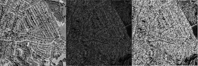
Figure 1.

A montage providing an example simulation of a SAR image (the amplitude modulations) before (centre) and after (right) histogram equalisation. The simulation is based on the application of an optical image (left) using the .m code provided in Appendix A for size = 1000 and width = 3. The result is predicated on Eq. (38), where the optical image is interpreted to be a map of the self-affine variations in the dielectric properties of the ground surface.

$$\left(\begin{array}{ccc}0& 1& 0\\ 1& -4& 1\\ 0& 1& 1\end{array}\right)$$

The optical image is normalised before application of the convolution operations with the Laplacian and PSF (using the MATLAB function conv2). The analytic signals are then computed using a Hilbert Transform (with MATLAB function hilbert) to simulate the quadrature detection process which occurs in range alone (in practice, this is coupled with demodulation). For a real function $f\left(x\right)$, the analytic signal is given by [4].

$$s\left(x\right)=f\left(x\right)+\mathit{i\pi x}{\otimes }_{x}f\left(x\right)$$E39

where the imaginary component is, by definition, the Hilbert transform of $f\left(x\right)$. However, the MATLAB function hilbert actually computes the analytic signal and not just the Hilbert transform (which is then given by the imaginary component of the function’s output).

The range and cross range directions given in Figure 1 are the vertical and horizontal components of the image, respectively. The simulated SAR image given in Figure 1 is normalised and histogram equalised [15] (using MATLAB function histeq) in order to enhance the dark field image features (which is a relatively standard practice in SAR image analysis).

The prototype MATLAB function used to generate this simulation—SARSIM—as given in the Appendix A is presented to allow interested readers to repeat the simulation for different input (8-bit grey level) images and control parameters, specifically the array length and the width of the sinc IRF. It provides the basis for further modifications associated with interrogating the processes used, and, as an aid to further improving the simulation based on refinements to the model conceived. This is discussed further in Section 12.1.

Figure 2 shows the IRF in range (and cross range), and a 256-bin histogram of the grey-levels for $I_{\mathrm{SAR}}\left(x,y\right)$—Eq. (38)—as given in Figure 1. The histogram is characteristic of a Rayleigh distribution which is the ‘signature distribution’ of a SAR image (and coherent images in general). The fact that the distribution of grey levels for $I_{\mathrm{SAR}}\left(x,y\right)$ is Rayleigh distributed can be quantified using the MATLAB function fitdist, for example, which returns the parameter value $B=0.0047$ for an assumed (and normalised) Rayleigh distribution given by

Figure 2.

The sinc IRF used to generate the SAR image simulation given in Figure 1 (left) and a 256-bin histogram of the amplitude modulations (normalised to values between 0 and 1) as shown in Figure 1 (right).

$$Pr\left[I_{\mathrm{SAR}}\left(x,y\right)\right]={\mathit{xB}}^{2}exp\left(-\frac{x^2}{2B^2}\right)$$

The simulation produces a result that is statistically compatible with a SAR image but with ‘structural features’ determined by those associated with the optical image. A simulation of this type must not be expected to provide a detailed resemblance of a real SAR image on a pixel-by-pixel basis. However, the structural and textural properties of the simulation may have similarities with a genuine SAR image, given that the ground surface is taken to be a Mandelbrot surface.

10.1 Texture simulation

A genuine SAR image is the product of a multitude of highly complex three-dimensional interactions (including polarisation effects), that transcend the model given by Eq. (38) based on the application of an areal optical image. However, in the context of assuming a fractal model for the ground surface, the approach considered provides a simulation that is at least texturally compatible with a real SAR image. In this respect, there are a range of texture comparators that can be used to assess the simulated image with respect to genuine data such as those given in [11], for example. It is a ‘solution’ to the problem of simulating SAR images that goes beyond the conventional approach of generating speckle patterns based on a weak point scattering model, for example [16]. Further, it may also provide value in terms of target detection (e.g. [17, 18]).

10.2 Target detection

Target detection is typically concerned with the interpretation of features in a SAR image that are isolated, but a with high intensities due to increased microwave back-scattering from objects that are conductors, for example, with a high Radar Cross Sections (RCS) [19]. In the context of the scalar EM field model considered here, to take into account back-scattering from conductive objects, we are required to consider a conductive dielectric model, and, more specifically, a scattering function where $\sigma \left(x,y\right)\cancel{=}0$ for specific locations. In this case, the scattered intensity (the RCS) can be expected to be significantly larger than that generated by variations is the relative permittivity alone [20]. This can be appreciated using an order of magnitude calculation as follows.

Consider a SAR with a wavelength of 1 cm, a relative permittivity for surface features with a Root Mean Square (RMS) value of $\sim 10$ say, and, an electrical conductivity for isolated metalic objects composed of steel, for example, with a RMS of $\sim {10}^6$ Siemens/metre. With reference to the definition of the scattering function given in Eq. (37), then, for a unit area of 1 square metre say, we can write (using the Minkowski inequality for a Euclidean norm)

$$\parallel \gamma \left(x,y,k_0\right){\parallel }_2\le \parallel {\gamma }_{\epsilon }\left(x,y\right){\parallel }_2+\frac{Z_0}{k_0}\parallel \sigma \left(x,y\right){\parallel }_2\simeq 10+0.6\times {10}^6=600010$$

which should be compared with $\sim 10$ for the case of a non-conductive dielectric and the same wavelength for the same unit area. In this respect, the simulation of a SAR image based on Eq. (38), may be used as a texture comparator with a genuine SAR image of the same area (for which an overhead aerial optical image is available) in order to identify conductive agents, should they exist in the a genuine SAR image.

In order to make such a comparator effective, the optical image can be median filtered to eradicate any form of salt-and-pepper noise (impulse noise), that may generate what appears to be isolated back-scattering events from conductive agents. This approach is most relevant to terrain that is relatively flat where conductive agents (such tanks and other military vehicles, for example) may be most likely to operate. Nevertheless, it should be noted that specular reflections from non-conductive dielectric features are capable of generating ‘false targets’. In the following section an approach to eradicating false targets is considered using a cross polarisation effect.

11. SAR image modelling with cross polarisation effects

Polarisation effects are compounded in solutions to Eq. (11). In regard to modelling a SAR image, we consider an approach where variations in the permittivity contribute significantly more to the cross polarisation effects of the electric field than do variations in the magnetic permeability. The purpose of this, is that it allows us to consider a reduced model based on the wave equation

$$\left({\nabla }^2+k^2\right)\mathbf{E}\left(\mathbf{r},k\right)=\gamma \left(\mathbf{r},k\right)\mathbf{E}\left(\mathbf{r},k\right)-\nabla \left[\mathbf{E}\left(\mathbf{r},k\right)\cdot \nabla ln\epsilon \left(\mathbf{r}\right)\right]$$

where it is assumed that ${\mu }_r\left(\mathbf{r}\right)\sim 1,\forall \mathbf{r}$. To implement the strong scattering solution to this equation, we note that Eq. (23) is also applicable for a vector field. i.e.

$$\left({\nabla }^2+k^2\right)\gamma \left(\mathbf{r},k\right){\mathbf{E}}_i\left(\mathbf{r},k\right)=0$$

given that this equation is valid for any scalar field component of the electric vector. Thus, we consider an equation for the strong scattering vector field ${\mathbf{E}}_s\left(\mathbf{r},k\right)$ in terms of the incident field ${\mathbf{E}}_i\left(\mathbf{r},k\right)$ given by

$$\left({\nabla }^2+k^2\right){\mathbf{E}}_s\left(\mathbf{r},k\right)=-1k^2{\nabla }^2\left[\gamma \left(\mathbf{r},k\right){\mathbf{E}}_i\left(\mathbf{r},k\right)\right]-\nabla \left[{\mathbf{E}}_i\left(\mathbf{r},k\right)\cdot \nabla ln\epsilon \left(\mathbf{r}\right)\right]$$E40

This equation only takes into account polarisation effects in the context of the Born approximation, which is, in effect, taken to be a second order effect compounded in the second term on the right hand side of Eq. (40). In this sense, Eq. (40) is a hybrid model for polarisation effects, although it is still possible to consider a solution for $E_s\left(\mathbf{r},k\right)$ with strong polarisation, given that we can write

$$\nabla \left[{\mathbf{E}}_i\left(\mathbf{r},k\right)\cdot \nabla ln{\epsilon }_r\left(\mathbf{r}\right)\right]=-\frac{1}{k^2}\nabla \left[\frac{{\nabla }^2\left[\gamma \left(\mathbf{r},k\right){\mathbf{E}}_i\left(\mathbf{r},k\right)\right]\gamma }{\left(\mathbf{r},k\right)}\cdot \nabla ln\epsilon \left(\mathbf{r}\right)\right]$$

Nevertheless, the analysis that follows is predicated on the hybrid model given by Eq. (40).

Using the same coordinate geometry considered in Section 8.1, we consider an incident vector field given by

$${\mathbf{E}}_i\left(\mathbf{r},k\right)=\widehat{\mathbf{z}}cos\varphi E_z\left(\mathbf{r},k\right)+\widehat{\mathbf{x}}sin\varphi E_x\left(\mathbf{r},k\right)\sim \widehat{\mathbf{z}}{E}_i\left(x,k\right)$$

where $E_i\left(x,k\right)$ is given by Eq. (31) and $\varphi \sim 0$ is the ‘Depression Angle’. The condition on the Depression Angle means that the approach that follows is only valid for relatively low Depression Angles which typically occur on military SAR platforms operating at a low altitudes and a long ranges. Moreover, the condition significantly helps to simplify the model in preparation for the analysis that follows, given that, Eq. (40), can now be written in the form

$$\left({\nabla }^2+k^2\right){\mathbf{E}}_s\left(\mathbf{r},k\right)=-\widehat{\mathbf{z}}\frac{1}{k^2}{\nabla }^2\left[\gamma \left(\mathbf{r},k\right)E_i\left(x,k\right)\right]-\nabla \left[E_i\left(x,k\right)\frac{\partial }{\partial z}ln\epsilon \left(\mathbf{r}\right)\right]$$

In this case, the scattered field that is measured in the same direction of polarisation as the incident field, denoted $E_{\mathit{sz}}\left(\mathbf{r},k\right)$, is given by the solution of

$$\left({\nabla }^2+k^2\right)E_{\mathit{sz}}\left(\mathbf{r},k\right)=-\frac{1}{k^2}{\nabla }^2\left[\gamma \left(\mathbf{r},k\right)E_i\left(x,k\right)\right]-\mathrm{\partial \partial }z\left[E_i\left(x,k\right)\frac{\partial }{\partial z}ln\epsilon \left(\mathbf{r}\right)\right]$$E41

This field are referred to as the VV (Vertical-Vertical) mode field. In addition to this, there is a cross-polarised scattered field, denoted by $E_{\mathit{sy}}\left(\mathbf{r},k\right)$, which is given by the solution of

$$\left({\nabla }^2+k^2\right)E_{\mathit{sy}}\left(\mathbf{r},k\right)=-\frac{\partial }{\partial y}\left[E_i\left(x,k\right)\frac{\partial }{\partial z}ln\epsilon \left(\mathbf{r}\right)\right]$$E42

and is referred to as the VH (Vertical-Horizontal) mode field.

11.1 Conditional solution

A condition which is of particular value in solving Eq. (41) and Eq. (42) using the methods presented in Section 8.1 is to consider the case when $ln\epsilon \left(\mathbf{r}\right)\sim \epsilon \left(\mathbf{r}\right)-1={\gamma }_{\epsilon }\left(\mathbf{r}\right)$ which is actually only valid for values of $\epsilon \left(\mathbf{r}\right)\sim 1,\forall \mathbf{r}$. Nevertheless, by repeating the analysis given in Section 8.1 (including application of exactly the same conditions), it can be shown that the equivalent solutions to Eq. (41) and Eq. (42) yield the following models for the real component of the processed SAR data (subject to application of a self-affine surface model as discussed in Section 9):

$$s_{\mathit{VV}}\left(x,y\right)=p\left(x,y\right){\otimes }_x{\otimes }_y{C}_1{\nabla }^2\gamma \left(x,y\right)$$

and

$$s_{\mathit{VH}}\left(x,y\right)=p\left(x,y\right){\otimes }_x{\otimes }_y{C}_3\frac{\partial }{\partial y}{\gamma }_{\epsilon }\left(x,y\right)$$

where

$$C_3=-k_0^2\underset{-\infty }{\overset{\infty }{\int }}\frac{\partial }{\partial z}\left[{\gamma }_{\epsilon }\left(z\right)\right]exp\left(-{\mathit{ik}}_0{z}_{0}z/x_0\right)\mathit{dz}=\frac{{\mathit{iz}}_0{k}_0^3}{x_0}\underset{-\infty }{\overset{\infty }{\int }}{\gamma }_{\epsilon }\left(z\right)exp\left(-{\mathit{ik}}_0{z}_{0}z/x_0\right)\mathit{dz}$$E43

Scaling both equations for $s_{\mathit{VV}}\left(x,y\right)$ and $s_{\mathit{VH}}\left(x,y\right)$ by $C_1{k}_0^2$, and redefining the conductivity as $\sigma \equiv Z_0\sigma /k_0$, we derived the data models

$$s_{\mathrm{VV}}\left(x,y\right)=p\left(x,y\right){\otimes }_x{\otimes }_y{\nabla }^2\left[-{\gamma }_{\epsilon }\left(x,y\right)+\mathit{i\sigma }\left(x,y\right)\right]$$E44

and

$$s_{\mathrm{VH}}\left(x,y\right)=p\left(x,y\right){\otimes }_x{\otimes }_y{\mathit{ik}}_0\frac{z_0}{x_0}\frac{\partial }{\partial y}{\gamma }_{\epsilon }\left(x,y\right)$$E45

The SAR images associated with these equation are given by

$$I_{\mathrm{VV}}\left(x,y\right)=\mid s_{\mathrm{VV}}\left(x,y\right)\mid \text{and}{I}_{\mathrm{VH}}\left(x,y\right)=\mid s_{\mathrm{VH}}\left(x,y\right)\mid$$

respectively, where, it is again presupposed, that the analytic signals have been generated in range for $s_{\mathrm{VV}}\left(x,y\right)$ and $s_{\mathrm{VH}}\left(x,y\right)$ before computation of the SAR images, thereby, providing display’s of the Amplitude Modulations.

11.2 Quantitative imaging

For a conductive dielectric, the scattering function is composed of two independent variables, namely ${\gamma }_{\epsilon }\left(x,y\right)$ and $\sigma \left(x,y\right)$. Consequently, a single VV SAR image is not able to quantitatively differentiate between these variables and can only rely on the expected increase in the RCS associated with a localised conductor in an other non-conductive dielectric environment to identify such a ‘target’. However, the VH data model given by Eq. (45) does not include the function $\sigma \left(x,y\right)$. In other words, according the model proposed, a SAR image based on the VH mode provides a measure of the variation in permittivity alone. Moreover, the models compounded in Eqs. (44) and (45), provide an option for quantitatively imaging the conductivity of the ground surface. This is important in the military applications of SAR, because isolated targets tend to be conductive agents due to the materials from which they are composed (assuming that stealth technologies have not been implemented).

From Eq. (45), we note that

$$s_{\mathit{VH}}^{\text{'}}\left(x,y\right)=\left(\frac{{\partial }^2}{\partial x^2}+\frac{\partial }{\partial y}\right)s_{\mathit{VH}}\left(x,y\right)=p\left(x,y\right){\otimes }_x{\otimes }_y{\mathit{ik}}_0{z}_0{x}_0{\nabla }^2{\gamma }_{\epsilon }\left(x,y\right)$$

Thus, using Eq. (44), we can write

$$I_{\mathrm{SAR}}^{\sigma }\left(x,y\right)=\left|{\mathit{ik}}_0\frac{z_0}{x_0}{s}_{\mathit{VV}}\left(x,y\right)+s_{\mathit{VH}}^{\text{'}}(x,y)\right|=\mid p\left(x,y\right){\otimes }_x{\otimes }_y{\nabla }^2\sigma \left(x,y\right)\mid$$E46

where $\sigma \equiv k_0{z}_0\sigma /x_0$. It should be noted that, for the case when the functions $s_{\mathrm{VV}}\left(x,y\right)$ and $s_{\mathrm{VH}}\left(x,y\right)$ are taken to be analytic (i.e. analytic signals in range $x$), then, using Eq. (39), Eq. (46) has the modified form

$$I_{\mathrm{SAR}}^{\sigma }\left(x,y\right)=\left|p\left(x,y\right){\otimes }_x{\otimes }_y\left[\frac{1}{\mathit{\pi x}}{\otimes }_x{\nabla }^2\sigma \left(x,y\right)\right]\right|$$

A simulation using Eqs. (44) and (45) and the data processing required to yield an image given by Eq. (46) is provided in Figure 3 for $k_0{z}_0/x_0=1$. For this example, an optical image of a port city has been chosen with a defined coastline. The simulated VV image $I_{\mathit{VV}}\left(x,y\right)$ is based on using Eq. (44) where

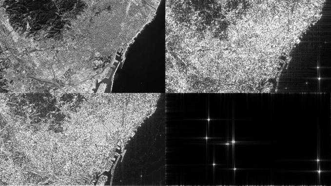
Figure 3.

Simulation of SAR images using the optical image (top left). The VV SAR image $I_{\mathit{VV}}\left(x,y\right)$ (top right) includes the effect of scattering from isolated targets. The VH SAR image $I_{\mathit{VH}}\left(x,y\right)$ (lower left) is based on the application of Eq. (45). Application of the Eq. (46) then yields the lower right hand image, which provides a quantitative image of the targets.

$${\gamma }_{\epsilon }\left(x,y\right)=I_{\text{Optical}}\left(x,y\right)+\mathit{i\sigma }\left(x,y\right)$$

for $I_{\text{Optical}}\in \left[0,1\right]$ and $\sigma \in \left[0,1\right]$. In the latter case, the function is taken to be zero except for some random and sparsely located ‘targets’ (when $\sigma =1$ for a small cluster of pixels). The simulated VH image $I_{\mathit{VH}}\left(x,y\right)$ is based on the application of Eq. (45) with $k_0{z}_0/x_0=1$. Application of the Eq. (46) then yields an image showing the location of the targets alone.

The simulations provided in Figure 3 are based on a modification of the code given in Appendix A. The cross range gradient given in Eq. (45) is computed using forward differencing through application of the MATLAB conv2 function; specifically, for image array I say, we apply I = conv2([1 -1], [1], I, ’same’). Thus, for compatibility with this process, the Laplacian is computed by applying the convolution process I = conv2([1 -1], [1 -1], I, ’same’) two-fold.

Any application of this quantitative imaging ‘solution’ using real SAR data requires Eq. (45) to be scaled by the (system specific) value of $z_0{k}_0/x_0$. For a 1 cm wavelength SAR, assuming that $z_0/x_0=k_0^{-1}$, as used for the simulation of $s_{\mathit{VH}}\left(x,y\right)$, implies a vary shallow depression angle of $\sim 2^{\mathrm{o}}$. An investigation into the use of different digital filters (using Finite Impulse Response and/or Fast Fourier Transform based filters) for computing the (digital) gradients is also necessary to determine an optimum data processing algorithm; research that lies beyond the scope of this work.

12. Summary and conclusions

The main contribution reported in this work is an application of the exact scattering solution developed in [5] to SAR image modelling. This solution cannot be used directly (in a generic sense) for modelling imaging systems (based on recording a scattered field) directly, but must be modified accordingly in relation to the physical configuration of the system, primarily the geometry and frequency of operation. In this regard, the strong scattering solution developed in Section 7 and then implemented for a SAR system in Section 8, provides a very simplified expression for modelling side band systems. In this case, the essential difference between a strong and weak scattering solution is quantified in terms of the use or otherwise of the Laplacian operator, respectively.

A fractal model for the scattering function has been introduced in Section 9. This allows a base band model to be considered, compounded in Eq. (36). An application of this solution has been considered whose aim is to provide a texturally compatible simulation of a SAR image for which a corresponding overhead aerial optical image is available. In this regard, some demonstratives examples have been provided based on the MATLAB code provided in Appendix A. The code is provide as a basis for the reader to repeat the simulations provided, and to further modify, improve and extend the code, subject to further developments of the model as considered in the following section.

12.1 Further developments

The reader will have observed that in evolving the model quantified by Eq. (36), a number of simplifications have been implemented. These are based on conditions that are reasonably compatible with a SAR system, at least, under certain operational conditions. They include, for example, a condition whereby the range is taken to be significantly larger than the operational height of the radar platform (i.e. $z_0/x_0<<1$). This is the basis for quantifying the relative contributions of terms whose scale is determined by the coefficients $C_1$, $C_2$ and $C_3$ given by Eqs. (32), (33) and (43), respectively. These coefficients are a result of introducing a separation of variables in regard to the scattering function $\gamma \left(x,y,z,k_0\right)$ as a function of height. It is key to generating a two-dimensional solution that is designed to be compatible with a SAR data, and relies on a model where $\gamma \left(z,k_0\right)\in \left(-\infty ,\infty \right)$. However, this model can be modified in order to introduce the effect of height variations, for example. Thus, suppose we consider the case where $\gamma \left(z,k_0\right)={\gamma }_0\in \left[0,h\left(x,y\right)\right]$ where ${\gamma }_0$ is a constant and $h\left(x,y\right)$ describes the variations in height of the surface at a point $\left(x,y\right)$ above a common based line $z=0$ say. Suppose $h\left(x,y\right)\in \left[0,1\right]\forall \left(x,y\right)$, then the integral over $\gamma \left(z,k_0\right)$ that is common to Eqs. (32), (33) and (43) is given by

$$\underset{0}{\overset{h\left(x,y\right)}{\int }}exp\left(-{\mathit{ik}}_0{z}_{0}z/x_0\right)\mathit{dz}=h\left(x,y\right)-i\frac{k_0{z}_0}{2x_0}{h}^2\left(x,y\right)+\dots \sim h\left(x,y\right)$$

Consequently, the strong scattering function ${\nabla }^2\gamma \left(x,y,k_0\right)$ can be replaced with $h\left(x,y\right){\nabla }^2\gamma \left(x,y,k_0\right)$. The incorporation of height variations in this way may be served in cases where a stereo optical image of the surface is available, for example.

This is just one example of other developments that can be considered to make the model increasingly more realistic, but necessarily more complicated, e.g. the inclusion of depression angles where $\varphi \in \left(0,\pi /2\right)$ radians, the inclusion of the second and third terms in Eq. (29), and using an incident field that includes the beam profile. In this respect, and, in addition to further developments of the model as discussed above, the relative simplicity of the result quantified in Eq. (38) can be further investigate through the introduction of additive stochastic fields [21] which are taken to account for the physical limitations of the model as well as ‘system noise’.

12.2 Final statement

The goal of attempting to simulate one imaging modality from another is becoming a common theme in imaging science, especially for applications in computer vision. This includes the simulation of one image from another whose physical formation and characteristics are entirely different.

Solutions to this problem can be used to help in the training of deep learning systems, for example [22]. In this context, the strong scattering solution developed in this paper, coupled with a fractal model for the scattering function, may provide an additional tool in the analysis and interpretation of SAR images. More generally, the solution may complement the processing of images formed from strong scattering interactions whose interpretation is undertaken using statistical modelling techniques alone (e.g. [23, 24]).

Acknowledgments

The author acknowledges the Science Foundation Ireland and the Technological University Dublin for supporting the Stokes Professorship program.

Conflict of interest

The author declares no conflict of interest.

Thanks

The author would like to thank Dr. Marek Rebow, Technological University Dublin for his continued support.

Appendix: MATLAB function for SAR image simulation

function SARSIM(size,width)%FUNCTION: SAR image simulation using optical images.%INPUTS: size - array length for computing the IRF.%width (>1) - width of IRF (sinc function).%OUTPUT: Display’s of three images in Figures 1–3.%Read optical image (default: 8-bit grey level image),I = imread(’filename’); %covert to double, normalise and show.I=double(im2gray(I)); I=I./max(max(I)); figure(1), imshow(I);%Define Laplacian filter and convolve it with the image.Laplace=[0 1 0; 1 -4 1; 0 1 0]; I=conv2(I, Laplace,’same’);%Compute the sinc function for inputs ’size’ and ’width’.x=round(size/2)-size:round(size/2); p=sinc(x/width);%Convolve data with the sinc function in range and%cross range, compute the analytic signals (columns)%with function hilbert and display Amplitude Modulations.s = conv2(p,p,I,’same’); s=hilbert(s); I = abs(s);I=I./max(max(I)); figure(2), imshow(I); %Display result.figure(3), imshow(histeq(I));%Apply histogram equalisation.

Nomenclature

EM	electromagnetic
IRF	impulse response function
PDF	probability density function
PSDF	power spectral density function
PSF	point spread function
RCS	radar cross section
RMS	root mean square
SAR	synthetic aperture radar
VV	vertical-vertical (polarisation)
VH	vertical-horizontal (polarisation)

References

- 1.
Harger RO. Synthetic Aperture Radar Systems: Theory and Design. New York: Academic Press; 1971 - 2.
Kovaly JJ. Synthetic Aperture Radar. London: Artech House; 1976. ISBN: 9780890060568 - 3.
Blackledge J. On the chirp function, the Chirplet transform and the optimal communication of information. IAENG International Journal of Applied Mathematics. 2020; 50 (2):285-319. Available from:https://arrow.tudublin.ie/engscheleart2/218/ [Accessed: August 22, 2023] - 4.
Blackledge JM. Digital Signal Processing (Second Edition). Cambridge: Woodhead Publishing; 2006. ISBN: 1-904275-26-5. Available from: https://arrow.tudublin.ie/engschelebk/4/ [Accessed: June 16, 2023] - 5.
Blackledge JM. A solution to the Schrödinger scattering problem. Mathematica Aeterna. 2015; 5 (2):273-283. Available from:https://www.longdom.org/articles-pdfs/a-solution-to-theschrodinger-scattering-problem.pdf [Accessed: July 3, 2023] - 6.
Jean-Claude Nédélec JC. The Helmholtz equation. In: Acoustic and Electromagnetic Equations: Integral Representations for Harmonic Problems. New York: Springer; 2001. pp. 9-109 - 7.
Evans GA, Blackledge JM, Yardley PD. Analytic Methods for Partial Differential Equations. In: Springer Undergraduate Mathematics Series (SUMS). Springer-Verlag Berlin and Heidelberg GmbH & Co. KG; 1999. ISBN: 9783540761242 - 8.
Hecht KT. The born approximation. In: Quantum Mechanics, Graduate Texts in Contemporary Physics. New York: Springer; 2000. [Online]. DOI: 10.1007/978-1-4612-1272-0 46 [Accessed: March 17, 2023] - 9.
Jones JA. Wave Conventions: The Good, the Bad and the Ugly. 2015. Available from: https://nmr.physics.ox.ac.uk/teaching/wavecon.pdf . [Accessed: September 17, 2023] - 10.
Mandelbrot B. The Fractal Geometry of Nature. New York: W. H. Freeman and Co.; 1982. ISBN: 0-7167-1186-9 - 11.
Turner MJ, Blackledge JM, Andrews P. Fractal Geometry in Digital Imaging. Cambridge, Massachusetts: Academic Press; 1998. ISBN: 0-12-703970-8 - 12.
Blackledge JM. A new definition, a generalisation and an approximation for a fractional derivative with applications to stochastic time series modelling. IAENG, Engineering Letters. 2021; 29 (1):138-150. Available from:https://arrow.tudublin.ie/engscheleart2/245/ [Accessed: August 21, 2023] - 13.
Marr D, Hildreth E. On the theory of edge detection. Proceedings of the Royal Society of London, Series B, Biological Sciences. 1980; 207 (1167):187-217. Available from:https://www.researchgate.net/publication/17083076_Theory_of_Edge_Detection [Accessed: August 22, 2023] - 14.
Blackledge J. A generalised nonlinear model for the evolution of low frequency freak waves. IAENG International Journal of Applied Mathematics. 2011; 41 (1):33-55. Available from:https://arrow.tudublin.ie/engscheleart2/41 [Accessed: August 21, 2023] - 15.
Blackledge JM. Digital image processing. Series in Electronic and Optical Materials. Cambridge: Woodhead Publishing; 2005. ISBN: 1-898563-49-7. Available from: https://arrow.tudublin.ie/engschelebk/3/ [Accessed: August 3, 2023] - 16.
Mitchell RL. Radar Signal Simulation. Massachusetts and London: Artech House, Inc.; 1976 - 17.
Shunjun W et al. HRSID: A high-resolution SAR images dataset for ship detection and instance segmentation. IEEE Access. 2020; 8 :120234-120254. Available from:https://ieeexplore.ieee.org/document/9127939 [Accessed: August 17, 2023] - 18.
Wang Y et al. A SAR dataset of ship detection for deep learning under complex backgrounds. Remote Sensing. 2019; 11 :765. DOI: 10.3390/rs11070765 - 19.
El-Darymli K, McGuire P, Power D, Moloney C. Target detection in synthetic aperture radar imagery: A state-of-the-art survey. Journal of Applied Remote Sensing. 2013; 7 (1):071598. Available from:https://arxiv.org/ftp/arxiv/papers/1804/1804.04719.pdf [Accessed: June 23, 2023] - 20.
Guo Q, Wang H, Xu F. Scattering enhanced attention pyramid network for aircraft detection in SAR images. IEEE Transactions on Geoscience and Remote Sensing. 2021; 59 (9):7570-7758. DOI: 10.1109/TGRS.2020.3027762 - 21.
Barton DK. Radar System Analysis and Modelling. London: Artech House; 2005. ISBN: 9781580536813 - 22.
Merkle N et al. Exploiting deep matching and SAR data for the geo-localization accuracy improvement of optical satellite images. Journal of Remote Sensing, MDPI. 2017; 9 (6). DOI: 10.3390/rs9060586. Available from:https://www.mdpi.com/2072-4292/9/6/586 [Accessed: June 24, 2023] - 23.
Korotkova O. Theoretical Statistical Optics. Singapore: World Scientific; 2021. ISBN-13: 9789811234972 - 24.
Frery AC, Wu J, Gomez L. SAR Image Analysis—A Computational Statistics Approach: With R Code, Data, and Applications. New Jersey: Wiley-IEEE Press; 2022. ISBN-10:111979529X