Dissolution of Porous Media and Underground Cavities: A Multi-Scale View

Abstract

To better understand the dissolution of porous media and underground cavities is very important in various applications. In this chapter, pore-scale dissolution model, which involves thermodynamic equilibrium or nonlinear reactive boundary conditions, is upscaled into Darcy-scale using the method of volume averaging. In the Darcy-scale model, several effective parameters are employed to describe the average behaviors of the pore-scale features, and they can be obtained by solving specific closure problems. The developed Darcy-scale model is validated by taking the dissolution of a gypsum pillar as an example. The results show that when Péclet and Reynolds number are within the assumptions to apply volume averaging, computation results using Darcy-scale model agree very well with direct numerical simulations. However, when they go beyond certain limits, 3D effects have to be taken into consideration.

1. Introduction

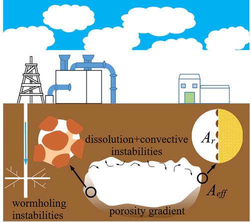
Dissolution of underground cavities and porous media are encountered in various subsurface processes, such as the evolution of karst formations [1], solutional salt mining [2], the geological sequestration of ${\mathrm{CO}}_2$ [3, 4], the improved oil recovery [5, 6, 7, 8], and so on. Many challenges we face in such problems relate to the crucial need of better description of reactive transport. Generally speaking, the evolution of underground cavities involves multiple scales. Figure 1 schematically shows the various scales associated to the injection of a dissolving fluid in a geological site (e.g., acid injection in oil recovery and solution mining of salt). On the one hand, it is possible to have the dissolution of a porous formation, which may lead to a porous dissolved region before the formation of a true fluid cavity. On the other hand, it may be the dissolution of an impervious rock formation with a more direct route to a fluid cavity. The heterogeneities generated during the process will make the multi-scale feature even more complicated [9].

Figure 1.

Schematic illustration of the multiple scales encountered in the dissolution of underground cavities.

It is a common sense that pore-scale model is the most accurate way to get deep insight into dissolution processes, in which the chemical-physical interactions take place and the full physics of dissolution is considered [10, 11, 12, 13]. In pore-scale modeling, the governing equations are solved with specific boundary conditions at the receding interfaces, without any assumption about the geometric structures of the porous media. And different phases are separated by the sharp interfaces [11, 12]. Such kind of pore-scale modeling was carried out using different methods, such as the Arbitrary-Lagrangian–Eulerian (ALE) framework [11, 14], level set method [15, 16], phase-field method [17], pore network models (PNM) [18, 19], and so on. However, pore-scale modeling is numerically difficult and expensive because of several reasons. Firstly, it is often very difficult to get the small-scale information, such as the structure of the skeleton and the voids. Secondly, people are more interested in large-scale behaviors in industrial or geological applications, which may range from decimeter to meter. However, to take all the microscopic pore-scale details into consideration is impractical and even impossible. Moreover, it is also a big chanllenge to explicitly treat the moving interface with large deformations, which may be created by the dissolution process [11, 13, 20]. To overcome this difficulty, an efficient way is to apply some sort of upscaling to the pore-scale models to study the dissolution problem from a macro-scale viewpoint. The macro-/Darcy-scale models filter pore-scale details below a cut-off length while representing them by several macro-scale effective parameters instead. These effective paramters can be solved through corresponding “closure problems” generated during the upscaling process. Since the middle of the last century, there appears a large number of studies on the upscaling of transport equations for a given chemical species. For example, the early fundamental works of Taylor [21, 22] and Aris [23] dealt with passive dispersion in porous media, i.e., advection and diffusion, without consideration of interaction at the fluid-solid interfaces. This problem was studied later using various upscaling tools [24, 25, 26], which led to the classical macro-scale dispersion theory and the proposition of local closure problems used to calculate the dispersion tensor components for various representative unit cells. An important progress was made by extending this theory to investigate active dispersion [27, 28, 29, 30], i.e., mass transport at the phase interface. Thereby, this led to the generation of an effective mass exchange term in the resulting Darcy-scale models, which incorporates the pore-scale thermodynamic equilibrium or reactive boundary condition at the interface [29].

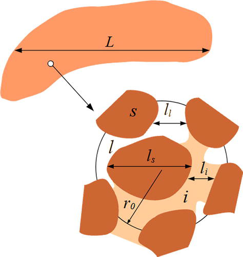
In this chapter, we consider a heterogeneous system as schematically illustrated in Figure 2. The pore-scale characteristic lengths are denoted as ${\mathrm{\ell }}_{\alpha }$, where $\alpha =l,i$ and s for the the liquid phase (in general water + dissolved species) flowing into the pore-space, the insoluble material, and the soluble material (which is assumed to contain only one component here), respectively. The macro-scale characteristic length is denoted as L. A third length-scale is defined as $r_0$, which is the radius of the representative elementary volume (REV). Upscaling can be done to develop a Darcy-scale model only when the hypothesis of scale separation expressed by

Figure 2.

Schematic illustration of the multiple scales associated with dissolution in a porous medium.

$${\mathrm{\ell }}_{\alpha }\ll r_0\ll L$$E1

is fulfilled.

The rest of this chapter is organized as follows. The pore-scale model to describe a dissolution problem will be presented at first. Then, volume averaging method will be used to upscale this pore-scale model into macro-scale. Closure problems used to solve the effective parameters emerging in the macro-scale model will be introduced subsequently and examples to show the validation and robustness of the macro-scale model will be given at last.

2. Pore-scale model

In this section, the pore-scale model is developed. The focus is on the mass transport problem, leaving aside the momentum and energy eqs. A hierarchical, multi-scale system is considered as schematically depicted in Figure 2. The momentum balance equations in the fluid phase are written as

$$\frac{\partial {\rho }_l{\mathbf{v}}_l}{\partial t}+{\rho }_l{\mathbf{v}}_l\cdot \nabla {\mathbf{v}}_l=-\nabla p_l+{\rho }_l\mathbf{g}+{\mu }_l{\nabla }^2{\mathbf{v}}_l\text{in\hspace{0.17em}\hspace{0.17em}the\hspace{0.17em}\hspace{0.17em}liquid\hspace{0.17em}\hspace{0.17em}phase}$$E2

$${\mathbf{v}}_l-{\mathbf{n}}_{\mathit{ls}}{\mathbf{n}}_{\mathit{ls}}\cdot {\mathbf{v}}_l=0\mathrm{at}{A}_{\mathit{ls}}$$E3

where ${\rho }_l$ is the liquid density, ${\mathbf{v}}_l$ the pore-scale liquid velocity, g the gravity, ${\mu }_l$ the dynamic viscosity, and $A_{\mathit{ls}}$ the interfacial area between the soluble solid and the liquid phase. For most underground dissolution processes, the density variation is negligible. For example, as the second most soluble rock, gypsum has a solubility in water of about 2.63 $\mathrm{kg}{\mathrm{m}}^{-3}$, which leads to the water density variation of less than 0.3%. However, when considering the dissolution of salt, buoyancy effects may be significant because of the large density variation. Nevertheless, considering the assumption that the liquid density is a constant, mass balance equations for the liquid phase and the dissolved species can be given by

$$\nabla \cdot {\mathbf{v}}_l=0\text{in\hspace{0.17em}\hspace{0.17em}the\hspace{0.17em}\hspace{0.17em}liquid\hspace{0.17em}\hspace{0.17em}phase}$$E4

$$\frac{\partial {\omega }_l}{\partial t}+{\mathbf{v}}_l\cdot \nabla {\omega }_l=\nabla \cdot \left(D_l\nabla {\omega }_l\right)\text{in\hspace{0.17em}\hspace{0.17em}the\hspace{0.17em}\hspace{0.17em}liquid\hspace{0.17em}\hspace{0.17em}phase}$$E5

with ${\omega }_l$ the mass fraction of the followed ion (e.g., ${\mathrm{Ca}}^{2+}$ in the context of gypsum dissolution) in the liquid phase and $D_l$ the molecular diffusion coefficient.

When considering a reactive boundary condition at the solid-liquid interface, the following kinetic condition can be written

$$\begin{array}{ll}{\mathbf{n}}_{\mathit{ls}}\cdot \left({\rho }_l{\omega }_l\left({\mathbf{v}}_l-{\mathbf{w}}_{\mathit{sl}}\right)-{\rho }_l{D}_l\nabla {\omega }_l\right)& =-M_c{k}_s{\left(1-\frac{{\omega }_l}{{\omega }_{\mathit{eq}}}\right)}^n\\ & ={\mathbf{n}}_{\mathit{ls}}\cdot \left({\rho }_s{\omega }_s\left({\mathbf{v}}_s-{\mathbf{w}}_{\mathit{sl}}\right)\right)\mathrm{at}{A}_{\mathit{ls}}\end{array}$$E6

In this equation, ${\rho }_s$ is the solid density, ${\omega }_s$ is the mass fraction of the followed component in the solid phase, ${\mathbf{v}}_s$ is the solid velocity, ${\mathbf{w}}_{\mathit{sl}}$ is the interface velocity, $M_c$ is the molar weight of the followed ion, $k_s$ is the reaction rate coefficient, and n is the nonlinear reaction order. The following boundary condition can be written from the mass balance of the solid phase

$$\begin{array}{ll}{\mathbf{n}}_{\mathit{ls}}\cdot \left({\rho }_s\left({\mathbf{v}}_s-{\mathbf{w}}_{\mathit{sl}}\right)\right)& ={\nu }_s{\mathbf{n}}_{\mathit{ls}}\cdot \left({\rho }_l{\omega }_l\left({\mathbf{v}}_l-{\mathbf{w}}_{\mathit{sl}}\right)-{\rho }_l{D}_l\nabla {\omega }_l\right)\\ & =-{\nu }_s{M}_c{k}_s{\left(1-\frac{{\omega }_l}{{\omega }_{\mathit{eq}}}\right)}^n\mathrm{at}{A}_{\mathit{ls}}\end{array}$$E7

where ${\nu }_s=M_s/M_c$ and $M_s$ is the molar weight of solid phase. The total mass balance boundary condition writes

$${\mathbf{n}}_{\mathit{ls}}\cdot \left({\rho }_l\left({\mathbf{v}}_l-{\mathbf{w}}_{\mathit{sl}}\right)\right)={\mathbf{n}}_{\mathit{ls}}\cdot \left({\rho }_s\left({\mathbf{v}}_s-{\mathbf{w}}_{\mathit{sl}}\right)\right)\mathrm{at}{A}_{\mathit{ls}}$$E8

In this chapter, the solid phase is assumed not moving, i.e., ${\mathbf{v}}_s=0$, thus ${\mathbf{v}}_s$ can be discarded in the boundary conditions. Consequently, Eqs. (7) and (8) can be transformed into

$${\mathbf{n}}_{\mathit{ls}}\cdot {\mathbf{w}}_{\mathit{sl}}={\rho }_s^{-1}{M}_s{k}_s{\left(1-\frac{{\omega }_l}{{\omega }_{\mathit{eq}}}\right)}^n\mathrm{at}{A}_{\mathit{ls}}$$E9

to calculate the interface velocity, and

$${\mathbf{n}}_{\mathit{ls}}\cdot {\rho }_l{\mathbf{v}}_l={\mathbf{n}}_{\mathit{ls}}\cdot \left({\rho }_l-{\rho }_s\right){\mathbf{w}}_{\mathit{sl}}=-\left(1-\frac{{\rho }_l}{{\rho }_s}\right)M_s{k}_s{\left(1-\frac{{\omega }_l}{{\omega }_{\mathit{eq}}}\right)}^n\mathrm{at}{A}_{\mathit{ls}}$$E10

to get the liquid velocity, respectively. Eqs. (7) and (8) also lead to

$${\mathbf{n}}_{\mathit{ls}}\cdot {\mathbf{w}}_{\mathit{sl}}=\frac{{\nu }_s}{{\rho }_s\left(1-{\nu }_s{\omega }_l\right)}{\mathbf{n}}_{\mathit{ls}}\cdot \left({\rho }_l{D}_l\nabla {\omega }_l\right)\mathrm{at}{A}_{\mathit{ls}}$$E11

in the case of an equilibrium condition, which provides a more convenient way to calculate the interface velocity. For gypsum dissolution, ${\mathbf{w}}_{\mathit{sl}}$ is in the order of ${10}^{-7}\mathrm{m}{\mathrm{s}}^{-1}$ and it is even smaller for the dissolution of carbonate rocks, which is usually negligible compared to the liquid velocity. Considering also Eq. (3), Eq. (6) can be simplified into

$${\mathbf{n}}_{\mathit{ls}}\cdot \left(-{\rho }_l{D}_l\nabla {\omega }_l\right)\approx -M_c{k}_s{\left(1-\frac{{\omega }_l}{{\omega }_{\mathit{eq}}}\right)}^n\mathrm{at}{A}_{\mathit{ls}}$$E12

Collect the above mass balance equations and boundary conditions, the pore-scale problem can be written as

$$\frac{\partial {\rho }_l}{\partial t}+\nabla \cdot \left({\rho }_l{\mathbf{v}}_l\right)=0\text{in\hspace{0.17em}the\hspace{0.17em}liquid\hspace{0.17em}phase}$$E13

$$\frac{\partial {\rho }_l{\omega }_l}{\partial t}+\nabla \cdot \left({\rho }_l{\omega }_l{\mathbf{v}}_l\right)=\nabla \cdot \left({\rho }_l{D}_l\nabla {\omega }_l\right)\text{in the liquid phase}$$E14

$${\mathbf{n}}_{\mathit{ls}}\cdot \left({\rho }_l{\omega }_l\left({\mathbf{v}}_l-{\mathbf{w}}_{\mathit{sl}}\right)-{\rho }_l{D}_l\nabla {\omega }_l\right)=-M_c{k}_s{\left(1-\frac{{\omega }_l}{{\omega }_{\mathit{eq}}}\right)}^n\mathrm{at}{A}_{\mathit{ls}}$$E15

$$\begin{array}{ll}{\mathbf{n}}_{\mathit{ls}}\cdot \left(-{\rho }_s{\mathbf{w}}_{\mathit{sl}}\right)& ={\mathbf{n}}_{\mathit{ls}}\cdot \left({\rho }_l\left({\mathbf{v}}_l-{\mathbf{w}}_{\mathit{sl}}\right)\right)\\ & ={\nu }_s{\mathbf{n}}_{\mathit{ls}}\cdot \left({\rho }_l{\omega }_l\left({\mathbf{v}}_l-{\mathbf{w}}_{\mathit{sl}}\right)-{\rho }_l{D}_l\nabla {\omega }_l\right)\\ & =-M_s{k}_s{\left(1-\frac{{\omega }_l}{{\omega }_{\mathit{eq}}}\right)}^n\mathrm{at}{A}_{\mathit{ls}}\end{array}$$E16

$$\frac{\partial {\rho }_s}{\partial t}=0\text{in the solid phase}$$E17

$${\mathbf{n}}_{\mathit{li}}\cdot \left({\rho }_l{\omega }_l{\mathbf{v}}_l-{\rho }_l{D}_l\nabla {\omega }_l\right)=0\mathrm{at}{A}_{\mathit{li}}$$E18

$${\mathbf{n}}_{\mathit{li}}\cdot {\mathbf{v}}_l=0\mathrm{at}{A}_{\mathit{li}}$$E19

Here, $A_{\mathit{li}}$ denotes the interfacial area between the insoluble solid and the liquid phase.

This pore-scale model should be completed with the momentum balance equations, such as Eqs. (2) and (3). Moreover, the momentum balance equations are independent of the mass balance equations, because the characteristic time for the relaxation of viscous flow is much shorter than the dissolution characteristic time, and the liquid velocity and viscosity are assumed constant. Thus, the focus of this chapter is on the mass transport problem.

Finally, when the boundary condition is thermodynamic equilibrium instead of the reactive condition discussed above, Eq. (15) should be replaced by

$${\omega }_l={\omega }_{\mathit{eq}}\mathrm{at}{A}_{\mathit{ls}}$$E20

3. Darcy-scale model

For the dissolution taking place in a porous medium such as illustrated in Figure 1, it is often not practical to take into account of all the pore-scale details by direct numerical modeling in a L-scale problem, even if this is the more secure way of handling the geometry evolution [10]. Consequently, attempts have been made to filter the pore-scale information below a cutoff length through upscaling techniques. In the past decades, several upscaling methods have been developed, such as volume averaging [31], ensemble averaging [32, 33], moments matching [34, 35], and multi-scale asymptotic [36]. In this section, the macro-scale model is developed using the technique of volume averaging, and this present work extends the contribution of Refs. [30, 37, 38].

3.1 Averages and averaged equations

The superficial and intrinsic average of the pore-scale liquid velocity, i.e., V and ${\mathbf{U}}_l$, are defined as

$${\mathbf{V}}_l=⟨{\mathbf{v}}_l⟩=\frac{1}{V}{\int }_{V_l}{\mathbf{v}}_l\mathit{dV}$$E21

and

$${\mathbf{U}}_l=\frac{1}{V_l}{\int }_{V_l}{\mathbf{v}}_l\mathit{dV}=\frac{{\mathbf{V}}_l}{{\epsilon }_l}$$E22

respectively, where V denotes the volume of the representative unit cell as illustrated in Figure 2, $V_l$ is the volume of the liquid phase within it, and ${\epsilon }_l$ is the porosity given by

$${\epsilon }_l=\frac{1}{V}{\int }_{V_l}\mathit{dV}$$E23

The intrinsic average of the mass fraction of the followed species in the liquid phase is written as

$${\mathrm{\Omega }}_l={⟨{\omega }_l⟩}^l=\frac{1}{V_l}{\int }_{V_l}{\omega }_l\mathit{dV}$$E24

The pore-scale and macro-scale variables are related through deviations by

$${\omega }_l={\mathrm{\Omega }}_l+{\tilde{\omega }}_l$$E25

$${\mathbf{v}}_l={\mathbf{U}}_l+{\tilde{\mathbf{v}}}_l$$E26

with ${\tilde{\omega }}_l$ and ${\tilde{\mathbf{v}}}_l$ representing the deviation of mass fraction of the followed component and the velocity of the liquid phase, respectively.

Averaging Eq. (13) leads to

$$\frac{\partial {\epsilon }_l{\rho }_l}{\partial t}+\nabla \cdot \left({\rho }_l{\mathbf{V}}_l\right)=-K_s$$E27

Here, the mass exchange term is given by

$$K_s=\frac{1}{V}\underset{A_{\mathit{ls}}}{\int }{\mathbf{n}}_{\mathit{ls}}\cdot {\rho }_l\left({\mathbf{v}}_l-{\mathbf{w}}_{\mathit{sl}}\right)\mathit{dA}$$E28

Applying average to the solid mass balance equation gives

$$\frac{\partial {\epsilon }_s{\rho }_s}{\partial t}=K_s$$E29

where Eq. (16) has been used to obtain

$$\begin{array}{ll}{K}_s= \frac{1}{V}{\int }_{A_{\mathit{ls}}}{\mathbf{n}}_{\mathit{ls}}\cdot \left(-{\rho }_s{\mathbf{w}}_{\mathit{sl}}\right)\mathit{dA}& =\frac{1}{V}{\int }_{A_{\mathit{ls}}}{\mathbf{n}}_{\mathit{ls}}\cdot {\rho }_l\left({\mathbf{v}}_l-{\mathbf{w}}_{\mathit{sl}}\right)\mathit{dA}\\ & =-a_{\mathit{vl}}{M}_s{k}_s{⟨{\left(1-\frac{{\omega }_l}{{\omega }_{\mathit{eq}}}\right)}^n⟩}_{\mathit{ls}}\end{array}$$E30

with the surface average and specific area defined as

$${⟨\star ⟩}_{\mathit{ls}}=\frac{1}{A_{\mathit{ls}}}\underset{A_{\mathit{ls}}}{\int }\star \mathit{dA}$$E31

and

$$a_{\mathit{vl}}=\frac{1}{V}\underset{A_{\mathit{ls}}}{\int }\mathit{dA}$$E32

respectively.

Finally, the mass balance equation for the followed ion writes

$$\begin{array}{l}\frac{\partial {\epsilon }_l{\rho }_l{\mathrm{\Omega }}_l}{\partial t}+\nabla \cdot \left({\epsilon }_l{\rho }_l{\mathrm{\Omega }}_l{\mathbf{U}}_l\right)+\underset{\text{dispersion}}{\underbrace{\nabla \cdot \left({\rho }_l⟨{\tilde{\omega }}_l{\tilde{\mathbf{v}}}_l⟩\right)}}=\\ \nabla \cdot \left({\epsilon }_l{\rho }_l{D}_l\nabla {\mathrm{\Omega }}_l+\underset{\text{tortuosity}}{\underbrace{\frac{1}{V}{\int }_{A_{\mathit{ls}}}{\mathbf{n}}_{\mathit{ls}}{\rho }_l{D}_l{\tilde{\omega }}_l\mathit{dA}+\frac{1}{V}{\int }_{A_{\mathit{li}}}{\mathbf{n}}_{\mathit{li}}{\rho }_l{D}_l{\tilde{\omega }}_l\mathit{dA}}}\right)-K_c\end{array}$$E33

The total mass exchange term $K_c$ is given by

$$K_c=\frac{M_c}{M_s}{K}_s=-a_{\mathit{vl}}{M}_c{k}_s{⟨{\left(1-\frac{{\omega }_l}{{\omega }_{\mathit{eq}}}\right)}^n⟩}_{\mathit{ls}}$$E34

Using Eq. (27), Eq. (33) can be written as

$$\begin{array}{l}{\epsilon }_l{\rho }_l\frac{\partial {\mathrm{\Omega }}_l}{\partial t}+{\epsilon }_l{\rho }_l{\mathbf{U}}_l\cdot \nabla {\mathrm{\Omega }}_l+\underset{\text{dispersion}}{\underbrace{\nabla \cdot \left({\rho }_l⟨{\tilde{\omega }}_l{\tilde{\mathbf{v}}}_l⟩\right)}}=\\ \nabla \cdot \left({\epsilon }_l{\rho }_l{D}_l\nabla {\mathrm{\Omega }}_l+\underset{\text{tortuosity}}{\underbrace{\frac{1}{V}{\int }_{A_{\mathit{ls}}}{\mathbf{n}}_{\mathit{ls}}{\rho }_l{D}_l{\tilde{\omega }}_l\mathit{dA}+\frac{1}{V}{\int }_{A_{\mathit{li}}}{\mathbf{n}}_{\mathit{li}}{\rho }_l{D}_l{\tilde{\omega }}_l\mathit{dA}}}\right)-K_c+K_s{\mathrm{\Omega }}_l\end{array}$$E35

3.2 Deviation equations and closure problems

Up to now, the equations are still macro- and micro-scale coupled, and we need to find out an estimation for the concentration deviations. This is done through the following steps. Firstly, substituting Eq. (25) into the pore-scale mass balance equations. Secondly, dividing the averaged equation (Eq. (35)) by ${\epsilon }_l$ and thirdly subtracting it from the pore-scale mass balance equations. It is noteworthy that the spatial variations of the volume fraction and liquid density over the REV are neglected. Using the following equations

$$\nabla \cdot \left({\rho }_l{\omega }_l{\mathbf{v}}_l\right)={\rho }_l{\omega }_l\nabla \cdot {\mathbf{v}}_l+{\rho }_l{\mathbf{v}}_l\cdot \nabla {\omega }_l={\rho }_l{\mathbf{v}}_l\cdot \nabla {\mathrm{\Omega }}_l+{\rho }_l{\mathbf{v}}_l\cdot \nabla {\tilde{\omega }}_l$$E36

$$\begin{array}{l}-{\epsilon }_l^{-1}\nabla \cdot \left({\epsilon }_l{\rho }_l{D}_l\nabla {\mathrm{\Omega }}_l+\frac{1}{V}{\int }_{A_{\mathit{ls}}}{\mathbf{n}}_{\mathit{ls}}{\rho }_l{D}_l{\tilde{\omega }}_l\mathit{dA}+\frac{1}{V}{\int }_{A_{\mathit{li}}}{\mathbf{n}}_{\mathit{li}}{\rho }_l{D}_l{\tilde{\omega }}_l\mathit{dA}\right)\approx \\ -\nabla \cdot \left({\rho }_l{D}_l\nabla {\mathrm{\Omega }}_l+\frac{{\epsilon }_l^{-1}}{V}{\int }_{A_{\mathit{ls}}}{\mathbf{n}}_{\mathit{ls}}{\rho }_l{D}_l{\tilde{\omega }}_l\mathit{dA}+\frac{{\epsilon }_l^{-1}}{V}{\int }_{A_{\mathit{li}}}{\mathbf{n}}_{\mathit{li}}{\rho }_l{D}_l{\tilde{\omega }}_l\mathit{dA}\right)\end{array}$$E37

$$\begin{array}{l}{\epsilon }_l^{-1}{K}_c-{\epsilon }_l^{-1}{K}_s{\mathrm{\Omega }}_l={\epsilon }_l^{-1}\frac{1}{V}{\int }_{A_{\mathit{ls}}}{\mathbf{n}}_{\mathit{ls}}\left({\rho }_l{\tilde{\omega }}_l\left({\mathbf{v}}_l-{\mathbf{w}}_{\mathit{sl}}\right)-{\rho }_l{D}_l\nabla {\tilde{\omega }}_l\right)\mathit{dA}\\ -{\rho }_l{D}_l{\epsilon }_l^{-1}\frac{1}{V}{\int }_{A_{\mathit{ls}}}{\mathbf{n}}_{\mathit{ls}}\mathit{dA}\cdot \nabla {\mathrm{\Omega }}_l\end{array}$$E38

$$\nabla \cdot \left(\frac{{\epsilon }_l^{-1}}{V}{\int }_{A_{\mathit{ls}}}{\mathbf{n}}_{\mathit{ls}}{\rho }_l{D}_l{\tilde{\omega }}_l\mathit{dA}+\frac{{\epsilon }_l^{-1}}{V}{\int }_{A_{\mathit{li}}}{\mathbf{n}}_{\mathit{li}}{\rho }_l{D}_l{\tilde{\omega }}_l\mathit{dA}\right)\ll \nabla \cdot \left({\rho }_l{D}_l\nabla {\tilde{\omega }}_l\right)$$E39

one obtains

$$\begin{array}{l}{\rho }_l\frac{\partial {\tilde{\omega }}_l}{\partial t}+{\rho }_l{\mathbf{v}}_l\cdot \nabla {\tilde{\omega }}_l+{\rho }_l{\tilde{\mathbf{v}}}_l\cdot \nabla {\mathrm{\Omega }}_l-{\epsilon }_l^{-1}\nabla \cdot \left({\rho }_l⟨{\tilde{\omega }}_l{\tilde{\mathbf{v}}}_l⟩\right)=\nabla \cdot \left({\rho }_l{D}_l\nabla {\tilde{\omega }}_l\right)\\ +\frac{{\epsilon }_l^{-1}}{V}{\int }_{A_{\mathit{ls}}}{\mathbf{n}}_{\mathit{ls}}\cdot {\rho }_l{\tilde{\omega }}_l\left({\mathbf{v}}_l-{\mathbf{w}}_{\mathit{sl}}\right)\mathit{dA}-\frac{{\epsilon }_l^{-1}}{V}{\int }_{A_{\mathit{ls}}}{\mathbf{n}}_{\mathit{ls}}\cdot {\rho }_l{D}_l\nabla {\tilde{\omega }}_l\mathit{dA}\\ -{\rho }_l{D}_l{\epsilon }_l^{-1}\frac{1}{V}{\int }_{A_{\mathit{ls}}}{\mathbf{n}}_{\mathit{ls}}\mathit{dA}\cdot \nabla {\mathrm{\Omega }}_l\end{array}$$E40

In addition, the assumption

$${\mathrm{\Omega }}_{\mathit{ls}}={⟨{\omega }_l⟩}_{\mathit{ls}}=\frac{1}{A_{\mathit{ls}}}{\int }_{A_{\mathit{ls}}}{\omega }_l\mathit{dA}\approx {\mathrm{\Omega }}_l$$E41

is used, so any integral of the form $\frac{1}{V}{\int }_{A_{\mathit{ls}}}{\omega }_l\mathit{dA}$ will be approximated by

$$\frac{1}{V}{\int }_{A_{\mathit{ls}}}{\omega }_l\mathit{dA}\approx a_{\mathit{vl}}{\mathrm{\Omega }}_l$$E42

Using Eq. (15), the boundary condition for the deviation can be written as

$$\begin{array}{l}{\mathbf{n}}_{\mathit{ls}}\cdot \left({\rho }_l{\mathrm{\Omega }}_l\left({\mathbf{v}}_l-{\mathbf{w}}_{\mathit{sl}}\right)\right)+{\mathbf{n}}_{\mathit{ls}}\cdot \left({\rho }_l{\tilde{\omega }}_l\left({\mathbf{v}}_l-{\mathbf{w}}_{\mathit{sl}}\right)\right)+{\mathbf{n}}_{\mathit{ls}}\cdot \left(-{\rho }_l{D}_l\nabla {\tilde{\omega }}_l\right)\\ +{\mathbf{n}}_{\mathit{ls}}\cdot \left(-{\rho }_l{D}_l\nabla {\mathrm{\Omega }}_l\right)=-M_c{k}_s{\left(1-\frac{{\mathrm{\Omega }}_l+{\tilde{\omega }}_l}{{\omega }_{\mathit{eq}}}\right)}^n\mathrm{at}{A}_{\mathit{ls}}\end{array}$$E43

The crucial assumption now, which will be tested quantitatively against DNS, is to estimate the nonlinear reaction rate by a first-order Taylor expansion, i.e.,

$$\begin{array}{l}{\mathbf{n}}_{\mathit{ls}}\cdot \left({\rho }_l{\mathrm{\Omega }}_l\left({\mathbf{v}}_l-{\mathbf{w}}_{\mathit{sl}}\right)\right)+{\mathbf{n}}_{\mathit{ls}}\cdot \left({\rho }_l{\tilde{\omega }}_l\left({\mathbf{v}}_l-{\mathbf{w}}_{\mathit{sl}}\right)\right)+{\mathbf{n}}_{\mathit{ls}}\cdot \left(-{\rho }_l{D}_l\nabla {\tilde{\omega }}_l\right)\\ +{\mathbf{n}}_{\mathit{ls}}\cdot \left(-{\rho }_l{D}_l\nabla {\mathrm{\Omega }}_l\right)=-M_c{k}_s{\left(1-\frac{{\mathrm{\Omega }}_l}{{\omega }_{\mathit{eq}}}\right)}^n+\frac{{\mathit{nM}}_c{k}_s}{{\omega }_{\mathit{eq}}}{\left(1-\frac{{\mathrm{\Omega }}_l}{{\omega }_{\mathit{eq}}}\right)}^{n-1}{\tilde{\omega }}_l\mathrm{at}{A}_{\mathit{ls}}\end{array}$$E44

or

$$\begin{array}{l}{\mathbf{n}}_{\mathit{ls}}\cdot \left({\rho }_l{\mathrm{\Omega }}_l\left({\mathbf{v}}_l-{\mathbf{w}}_{\mathit{sl}}\right)\right)+{\mathbf{n}}_{\mathit{ls}}\cdot \left({\rho }_l{\tilde{\omega }}_l\left({\mathbf{v}}_l-{\mathbf{w}}_{\mathit{sl}}\right)\right)+{\mathbf{n}}_{\mathit{ls}}\cdot \left(-{\rho }_l{D}_l\nabla {\tilde{\omega }}_l\right)\\ +{\mathbf{n}}_{\mathit{ls}}\cdot \left(-{\rho }_l{D}_l\nabla {\mathrm{\Omega }}_l\right)=-\frac{M_c{k}_s}{{\omega }_{\mathit{eq}}}{\left(1-\frac{{\mathrm{\Omega }}_l}{{\omega }_{\mathit{eq}}}\right)}^{n-1}\left({\omega }_{\mathit{eq}}-{\mathrm{\Omega }}_l-n{\tilde{\omega }}_l\right)\mathrm{at}{A}_{\mathit{ls}}\end{array}$$E45

Similarly, Eq. (18) gives

$${\mathbf{n}}_{\mathit{li}}\cdot \left(-{\rho }_l{D}_l\nabla {\tilde{\omega }}_l\right)+{\mathbf{n}}_{\mathit{li}}\cdot \left(-{\rho }_l{D}_l\nabla {\mathrm{\Omega }}_l\right)=0\mathrm{at}{A}_{\mathit{li}}$$E46

Following the developments described in the literature [30, 37, 38], $\left({\mathrm{\Omega }}_l-{\omega }_{\mathit{eq}}\right)$ and $\nabla {\mathrm{\Omega }}_l$ appeared in the above governing equations can be considered as source terms because they can be generated from the deviation terms. The mathematical structure of the above macro- and micro-scale coupled equations enables to write an approximate solution, using the expansion of the source terms and their higher derivatives as follows

$${\tilde{\omega }}_l=s_l\left({\mathrm{\Omega }}_l-{\omega }_{\mathit{eq}}\right)+{\mathbf{b}}_l\cdot \nabla {\mathrm{\Omega }}_l+\dots$$E47

which gives for the first-order derivatives

$$\nabla {\tilde{\omega }}_l=\nabla s_l\left({\mathrm{\Omega }}_l-{\omega }_{\mathit{eq}}\right)+\left(\nabla {\mathbf{b}}_l+s_l\mathbf{I}\right)\cdot \nabla {\mathrm{\Omega }}_l+\dots$$E48

According to the length-scale constraints $l_s,l_i,l_l\ll r_0\ll L$, terms involving higher-order derivatives than $\nabla {\mathrm{\Omega }}_l$ in Eq. (48) can be neglected. Substituting Eqs. (47) and (48) into Eq. (40), collecting terms for $\left({\mathrm{\Omega }}_l-{\omega }_{\mathit{eq}}\right)$ and $\nabla {\mathrm{\Omega }}_l$ and then employing the fundamental lemma stated in Ref. [30], two closure problems shown below were obtained, which are dependent on the macro-scale mass fraction ${\mathrm{\Omega }}_l$.

Problem I:

$${\rho }_l\frac{\partial s_l}{\partial t}+{\rho }_l{\mathbf{v}}_l\cdot \nabla s_l=\nabla \cdot \left({\rho }_l{D}_l\nabla s_l\right)+{\epsilon }_l^{-1}{\rho }_l{X}_l\text{in the liquid phase}$$E49

$$\begin{array}{l}{\mathbf{n}}_{\mathit{ls}}\cdot \frac{{\mathrm{\Omega }}_l}{{\mathrm{\Omega }}_l-{\omega }_{\mathit{eq}}}{\rho }_l\left({\mathbf{v}}_l-{\mathbf{w}}_{\mathit{sl}}\right)+{\mathbf{n}}_{\mathit{ls}}\cdot \left({\rho }_l{s}_l\left({\mathbf{v}}_l-{\mathbf{w}}_{\mathit{sl}}\right)-{\rho }_l{D}_l\nabla s_l\right)\\ =\frac{M_c{k}_s}{{\omega }_{\mathit{eq}}}{\left(1-\frac{{\mathrm{\Omega }}_l}{{\omega }_{\mathit{eq}}}\right)}^{n-1}\left(1+n{s}_l\right)\mathrm{at}{A}_{\mathit{ls}}\left(t\right)\end{array}$$E50

$${\mathbf{n}}_{\mathit{li}}\cdot \left(-{\rho }_l{D}_l\nabla s_l\right)=0\mathrm{at}{A}_{\mathit{li}}$$E51

$$⟨s_l⟩=0\text{in the liquid phase}$$E52

$$s_l\left(\mathbf{x}+{\mathbf{l}}_i\right)=s_l\left(\mathbf{x}\right)$$E53

here, $A_{\mathit{ls}}\left(t\right)$ was used to indicate the geometry evolution and the following notations were defined

$$\begin{array}{ll}{\rho }_l{X}_l=& \frac{1}{V}{\int }_{A_{\mathit{ls}}}{\mathbf{n}}_{\mathit{ls}}\cdot {\rho }_l{s}_l\left({\mathbf{v}}_l-{\mathbf{w}}_{\mathit{sl}}\right)\mathit{dA}-\frac{1}{V}{\int }_{A_{\mathit{ls}}}{\mathbf{n}}_{\mathit{ls}}\cdot {\rho }_l{D}_l\nabla s_l\mathit{dA}\\ & -\frac{1}{V}{\int }_{A_{\mathit{li}}}{\mathbf{n}}_{\mathit{li}}\cdot {\rho }_l{D}_l\nabla s_l\mathit{dA}\end{array}$$E54

Making average to Eq. (49) and considering ${\rho }_l⟨{\mathbf{v}}_l\cdot \nabla s_l⟩={\rho }_l\nabla \cdot ⟨{\mathbf{v}}_l{s}_l⟩=0$, we can write

$$\begin{array}{ll}{\rho }_l\frac{\partial ⟨s_l⟩}{\partial t}=& -\frac{1}{V}{\int }_{A_{\mathit{ls}}}{\mathbf{n}}_{\mathit{ls}}\cdot {\rho }_l{s}_l\left({\mathbf{v}}_l-{\mathbf{w}}_{\mathit{sl}}\right)\mathit{dA}+\frac{1}{V}{\int }_{A_{\mathit{ls}}}{\mathbf{n}}_{\mathit{ls}}\cdot {\rho }_l{D}_l\nabla s_l\mathit{dA}\\ & +\frac{1}{V}{\int }_{A_{\mathit{li}}}{\mathbf{n}}_{\mathit{li}}\cdot {\rho }_l{D}_l\nabla s_l\mathit{dA}+{\rho }_l{X}_l\equiv 0\end{array}$$E55

which confirms the consistency of the proposed closure problem.

Problem II:

$${\rho }_l\frac{\partial {\mathbf{b}}_l}{\partial t}+{\rho }_l{\mathbf{v}}_l\cdot \left(\nabla {\mathbf{b}}_l+s_l\mathbf{I}\right)+{\rho }_l{\tilde{\mathbf{v}}}_l-{\epsilon }_l^{-1}{\rho }_l⟨{\tilde{\mathbf{v}}}_l{s}_l⟩=\nabla \cdot \left({\rho }_l{D}_l\left(\nabla {\mathbf{b}}_l+s_l\mathbf{I}\right)\right)+{\epsilon }_l^{-1}{\rho }_l{\mathbf{u}}_l\text{in}\text{the}\text{liquid}\text{phase}$$E56

$$\begin{array}{l}{\mathbf{n}}_{\mathit{ls}}\cdot \left({\rho }_l\left({\mathbf{v}}_l-{\mathbf{w}}_{\mathit{sl}}\right){\mathbf{b}}_l-{\rho }_l{D}_l\left(\nabla {\mathbf{b}}_l+s_l\mathbf{I}\right)\right)-{\rho }_l{D}_l{\mathbf{n}}_{\mathit{ls}}\\ =n\frac{M_c{k}_s}{{\omega }_{\mathit{eq}}}{\left(1-\frac{{\mathrm{\Omega }}_l}{{\omega }_{\mathit{eq}}}\right)}^{n-1}{\mathbf{b}}_l\mathrm{at}{A}_{\mathit{ls}}\left(t\right)\end{array}$$E57

$${\mathbf{n}}_{\mathit{li}}\cdot \left(-{\rho }_l{D}_l\left(\nabla {\mathbf{b}}_l+s_l\mathbf{I}\right)\right)={\rho }_l{D}_l{\mathbf{n}}_{\mathit{li}}\mathrm{at}{A}_{\mathit{li}}$$E58

$$⟨{\mathbf{b}}_l⟩=0\text{in}{V}_l$$E59

$${\mathbf{b}}_l\left(\mathbf{x}+{\mathbf{l}}_i\right)={\mathbf{b}}_l\left(\mathbf{x}\right)$$E60

in which

$$\begin{array}{l}{\rho }_l{\mathbf{u}}_l=\frac{1}{V}{\int }_{A_{\mathit{ls}}}{\mathbf{n}}_{\mathit{ls}}\cdot {\rho }_l\left({\mathbf{v}}_l-{\mathbf{w}}_{\mathit{sl}}\right){\mathbf{b}}_l\mathit{dA}-\frac{1}{V}{\int }_{A_{\mathit{ls}}}{\mathbf{n}}_{\mathit{ls}}\cdot {\rho }_l{D}_l\left(\nabla {\mathbf{b}}_l+s_l\mathbf{I}\right)\\ -\frac{1}{V}{\int }_{A_{\mathit{ls}}}{\mathbf{n}}_{\mathit{ls}}{\rho }_l{D}_l\mathit{dA}\end{array}$$E61

Using the following relation

$$-\nabla {\epsilon }_l=\frac{1}{V}{\int }_{A_{\mathit{ls}}}{\mathbf{n}}_{\mathit{ls}}\mathit{dA}+\frac{1}{V}{\int }_{A_{\mathit{li}}}{\mathbf{n}}_{\mathit{li}}\mathit{dA}=0$$E62

it may be written that

$$-\frac{1}{V}{\int }_{A_{\mathit{ls}}}{\mathbf{n}}_{\mathit{ls}}{\rho }_l{D}_l\mathit{dA}=\frac{1}{V}{\int }_{A_{\mathit{li}}}{\mathbf{n}}_{\mathit{li}}{\rho }_l{D}_l\mathit{dA}$$E63

which becomes

$$-\frac{1}{V}{\int }_{A_{\mathit{ls}}}{\mathbf{n}}_{\mathit{ls}}{\rho }_l{D}_l\mathit{dA}=-\frac{1}{V}{\int }_{A_{\mathit{li}}}{\mathbf{n}}_{\mathit{li}}\cdot \left({\rho }_l{D}_l\left(\nabla {\mathbf{b}}_l+s_l\mathbf{I}\right)\right)\mathit{dA}$$E64

because of Eq. (58). Then, Eq. (61) may be recast into a more convenient form

$$\begin{array}{c}{\rho }_l{\mathbf{u}}_l=\frac{1}{V}{\int }_{A_{\mathit{ls}}}{\mathbf{n}}_{\mathit{ls}}\cdot {\rho }_l\left({\mathbf{v}}_l-{\mathbf{w}}_{\mathit{sl}}\right){\mathbf{b}}_l\mathit{dA}-\frac{1}{V}{\int }_{A_{\mathit{ls}}}{\mathbf{n}}_{\mathit{ls}}\cdot {\rho }_l{D}_l\left(\nabla {\mathbf{b}}_l+s_l\mathbf{I}\right)\mathit{dA}\\ -\frac{1}{V}{\int }_{A_{\mathit{li}}}{\mathbf{n}}_{\mathit{li}}\cdot {\rho }_l{D}_l\left(\nabla {\mathbf{b}}_l+s_l\mathbf{I}\right)\mathit{dA}\end{array}$$E65

which can be used to check the consistency relationship

$${\rho }_l\frac{\partial ⟨{\mathbf{b}}_l⟩}{\partial t}\equiv 0$$E66

In the above closure problems, the zero average conditions on $s_l$ and ${\mathbf{b}}_l$ make sure that the deviation of the mass fraction is zero. The initial conditions are essential to make the problem complete, but they are still not specified. Since they are dependent on the specific problem to be solved in the transient case, while in the fllowing we only consider the steady-state behavior, this discussion is left open here.

We can notice that the two problems are still coupled by the terms involving $s_l$. It is believed essential to keep such a coupling to better estimate the flux exchange. Up to this point, the interface velocity has been kept in the equations, which makes the mass balance equations consistent. However, if we want to solve these problems, the interface position, interface velocity, and the macro-scale mass fraction have to be known properties. Assuming that mass fluxes near the interface are triggered by the diffusive flux, which is acceptable in most dissolution problems, approximate closure problems may be developed as done in Ref. [29].

3.3 Macro-scale equations and effective parameters

Substituting the deviation of the mass fraction Eq. (47) in the averaged equation Eq. (33), we get

$$\begin{array}{l}\frac{\partial {\epsilon }_l{\rho }_l{\mathrm{\Omega }}_l}{\partial t}+\nabla \cdot \left({\epsilon }_l{\rho }_l{\mathrm{\Omega }}_l{\mathbf{U}}_l\right)+\nabla \cdot \left({\rho }_l⟨{\tilde{\mathbf{v}}}_l{s}_l⟩\left({\mathrm{\Omega }}_l-{\omega }_{\mathit{eq}}\right)+{\rho }_l⟨{\tilde{\mathbf{v}}}_l{\mathbf{b}}_l⟩\cdot \nabla {\mathrm{\Omega }}_l\right)\\ =\nabla \cdot \left({\epsilon }_l{\rho }_l{D}_l\nabla {\mathrm{\Omega }}_l\right)+\nabla \cdot \left(\frac{1}{V}{\int }_{A_{\mathit{ls}}}{\mathbf{n}}_{\mathit{ls}}{\rho }_l{D}_l\left({\mathbf{b}}_l\cdot \nabla {\mathrm{\Omega }}_l+s_l\left({\mathrm{\Omega }}_l-{\omega }_{\mathit{eq}}\right)\right)\mathit{dA}\right)\\ +\nabla \cdot \left(\frac{1}{V}{\int }_{A_{\mathit{li}}}{\mathbf{n}}_{\mathit{li}}{\rho }_l{D}_l\left({\mathbf{b}}_l\cdot \nabla {\mathrm{\Omega }}_l+s_l\left({\mathrm{\Omega }}_l-{\omega }_{\mathit{eq}}\right)\right)\mathit{dA}\right)-K_c\end{array}$$E67

with $K_c$ defined by Eq. (34).

It is convenient to write Eq. (67) under the form of a generalized dispersion equation such as

$$\frac{\partial {\epsilon }_l{\rho }_l{\mathrm{\Omega }}_l}{\partial t}+\nabla \cdot \left({\epsilon }_l{\rho }_l{\mathrm{\Omega }}_l{\mathbf{U}}_l+{\epsilon }_l{\rho }_l\left({\mathrm{\Omega }}_l-{\omega }_{\mathit{eq}}\right){\mathbf{U}}_l^{\ast }\right)=\nabla \cdot \left({\epsilon }_l{\rho }_l{\mathbf{D}}_l^{\ast }\cdot \nabla {\mathrm{\Omega }}_l\right)-K_c$$E68

with the dispersion tensor given by

$${\mathbf{D}}_l^{\ast }=D_l\left(\mathbf{I}+\frac{1}{V_l}{\int }_{A_{\mathit{ls}}}{\mathbf{n}}_{\mathit{ls}}{\mathbf{b}}_l\mathit{dA}+\frac{1}{V_l}{\int }_{A_{\mathit{li}}}{\mathbf{n}}_{\mathit{li}}{\mathbf{b}}_l\mathit{dA}\right)-{⟨{\tilde{\mathbf{v}}}_l{\mathbf{b}}_l⟩}^l$$E69

and the non-traditional effective velocity given by

$${\mathbf{U}}_l^{\ast }={⟨{\tilde{\mathbf{v}}}_l{s}_l⟩}^l-\frac{1}{V_l}{\int }_{A_{\mathit{ls}}}{\mathbf{n}}_{\mathit{ls}}{D}_l{s}_l\mathit{dA}-\frac{1}{V_l}{\int }_{A_{\mathit{li}}}{\mathbf{n}}_{\mathit{li}}{D}_l{s}_l\mathit{dA}$$E70

The mass exchange term can be calculated as (neglecting higher-order derivatives than $\nabla {\mathrm{\Omega }}_l$)

$$\begin{array}{ll}{K}_c=& {\mathrm{\Omega }}_{\mathit{ls}}{K}_s+\left({\mathrm{\Omega }}_l-{\omega }_{\mathit{eq}}\right)\frac{1}{V}{\int }_{A_{\mathit{ls}}}{\mathbf{n}}_{\mathit{ls}}\cdot \left({\rho }_l{s}_l\left({\mathbf{v}}_l-{\mathbf{w}}_{\mathit{sl}}\right)-{\rho }_l{D}_l\nabla s_l\right)\mathit{dA}\\ & +\left(\frac{1}{V}{\int }_{A_{\mathit{ls}}}{\mathbf{n}}_{\mathit{ls}}\cdot \left({\rho }_l\left({\mathbf{v}}_l-{\mathbf{w}}_{\mathit{sl}}\right){\mathbf{b}}_l-{\rho }_l{D}_l\left(\nabla {\mathbf{b}}_l+s_l\mathbf{I}\right)\right)\mathit{dA}\right)\cdot \nabla {\mathrm{\Omega }}_l\\ & -{\rho }_l{D}_l\left(\frac{1}{V}{\int }_{A_{\mathit{ls}}}{\mathbf{n}}_{\mathit{ls}}\mathit{dA}\right)\cdot \nabla {\mathrm{\Omega }}_l\end{array}$$E71

This equation is important because it illustrates the structure of the mass exchange term, no mater the boundary condition is reactive or thermodynamic equilibrium. Particularly, it indicates that the mass exchange term is dependent on both the the averaged concentration and its gradient. Moreover, if relate this term to the reaction rate expression of Eq. (34), we obtain the expression below

$$K_c=-a_{\mathit{vl}}{M}_c{k}_s{⟨{\left(1-\frac{{\mathrm{\Omega }}_l+s_l\left({\mathrm{\Omega }}_l-{\omega }_{\mathit{eq}}\right)+{\mathbf{b}}_l\cdot \nabla {\mathrm{\Omega }}_l}{{\omega }_{\mathit{eq}}}\right)}^n⟩}_{\mathit{ls}}$$E72

Like Eq. (45), the linearized version can be written as

$$K_c=-a_{\mathit{vl}}\frac{M_c{k}_s}{{\omega }_{\mathit{eq}}}{\left(1-\frac{{\mathrm{\Omega }}_l}{{\omega }_{\mathit{eq}}}\right)}^{n-1}\left({\omega }_{\mathit{eq}}-{\mathrm{\Omega }}_l-n{\mathrm{\Omega }}_{\mathit{ls}}\right)$$E73

or

$$K_c=-a_{\mathit{vl}}{M}_c{\left(1-\frac{{\mathrm{\Omega }}_l}{{\omega }_{\mathit{eq}}}\right)}^n{k}_{s,\mathit{eff}}+a_{\mathit{vl}}{M}_c{\left(1-\frac{{\mathrm{\Omega }}_l}{{\omega }_{\mathit{eq}}}\right)}^{n-1}{\mathbf{h}}_l^{\ast }\cdot \nabla {\mathrm{\Omega }}_l$$E74

where the effective reaction rate coefficient is given by

$$k_{s,\mathit{eff}}=k_s\left(1+n{⟨s_l⟩}_{\mathit{ls}}\right)$$E75

in a similar form as in Ref. [39] for the first-order reaction case. The additional gradient term coefficient is

$${\mathbf{h}}_l^{\ast }=n\frac{k_s}{{\omega }_{\mathit{eq}}}{⟨{\mathbf{b}}_l⟩}_{\mathit{ls}}$$E76

One must remember that the macro-scale problem also involves the following averaged equations

$$\frac{\partial {\epsilon }_l{\rho }_l}{\partial t}+\nabla \cdot \left({\rho }_l{\mathbf{V}}_l\right)=-K_s,\frac{\partial {\epsilon }_s{\rho }_s}{\partial t}=K_s$$E77

The resulting macro-scale model is a generalization to nonlinear reaction rates of non-equilibrium models previously published. Such models are useful in many circumstances, for instance as diffuse interface models for modeling the dissolution of cavities [11, 40] or for studying instability of dissolution fronts [5].

4. Numerical examples

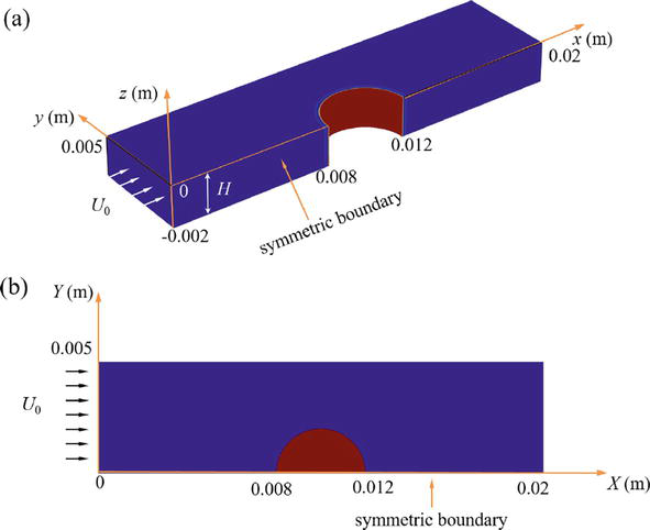
In this section, we validate the Darcy-scale model developed in the above section using the dissolution of a pillar located in a Hele-Shaw structure as an example and the computations were performed with the finite element software COMSOL Multiphysics^®. Only half of the symmetric geometries were used in the simulations for the sake of simplicity, as presented in Figure 3. In the direct numerical simulations using the pore-scale model, the geometry is three-dimensional as shown in Figure 3(a), with Poiseuille flow (average velocity of $U_0$) and zero mass fraction at the inlet (left surface), thermodynamic equilibrium mass fraction and no-slip boundary condition at the pillar surface (curved), zero mass flux and no-slip boundary conditions at the top, bottom and back surfaces, convective flux, and zero pressure at the outlet (right surface). After vertical averaging, the 3D geometry became 2D as presented in Figure 3(b). Moreover, the whole medium was considered as a continuum in Darcy-scale model, different from at pore-scale that the solid and liquid spaces were considered separately. The pore-scale boundary condition at the solid/fluid interface was incorporated into the effective parameters when upscaled into Darcy-scale. Therefore, boundary conditions were only prescribed for other borders and they were the same as done in pore-scale modeling. In some previous studies [1, 12, 41], it was demonstrated that Darcy-Brinkmann equation

Figure 3.

The 3D geometry used for the DNS (a) and the 2D geometry used for the macro-scale model (b).

$$-\left(\nabla P_l-{\rho }_l\mathbf{g}\right)+{\mu }_l^{\ast }{\nabla }^2{\mathbf{V}}_l-{\mu }_l{\mathbf{K}}_l^{-1}\cdot {\mathbf{V}}_l=0$$E78

is a better choice of the macro-scale momentum equation than Darcy’s law, because it includes both a viscous and a Darcy term. When the permeability tends to infinity the equation simplifies to Stokes equation

$$-\left(\nabla P_l-{\rho }_l\mathbf{g}\right)+{\mu }_l^{\ast }{\nabla }^2{\mathbf{V}}_l=0$$E79

and when the permeability is small enough Darcy’s equation is recovered

$${\mathbf{V}}_l=-\frac{{\mathbf{K}}_l}{{\mu }_l}\cdot \left(\nabla P_l-{\rho }_l\mathbf{g}\right)$$E80

For the computations of these two systems, without losing generality, we use pure gypsum dissolution in water as an example while it could also be other soluble materials, such as halite and carbonates in geological structures. The parameters used are presented in Table 1 and the thermodynamic equilibrium mass fraction of the followed ${\mathrm{Ca}}^{2+}$ is estimated as

Parameter	Value
${\rho }_l$	1000 $\mathrm{kg}{\mathrm{m}}^{-3}$
${\rho }_s$	2310 $\mathrm{kg}{\mathrm{m}}^{-3}$
${\mu }_l$	${10}^{-3}$ Pa s
$D_l$	${10}^{-9}{\mathrm{m}}^2{\mathrm{s}}^{-1}$
$L_r$	2 mm

Table 1.

Simulation parameters.

$${\omega }_{\mathit{eq}}=M_{\mathit{Ca}}\left(1.32\times {10}^{-2}+1.31\times {10}^{-4}T-1.47\times {10}^{-6}{T}^2\right)$$E81

where $M_{\mathit{Ca}}$ is the molar weight of Ca and T is the common temperature in $°\mathrm{C}$.

To describe the conditions used for the simulations, we introduce Darcy-scale Reynolds number ${Re}_M$ and Péclet number ${\mathrm{Pe}}_M$, i.e.,

$${Re}_M=\frac{{\rho }_r{U}_0{L}_r}{{\mu }_l};{\mathrm{Pe}}_M=\frac{U_0{L}_r}{D_l}$$E82

where $L_r$ is a characteristic length such as the aperture of the Hele-Shaw structure. These two dimensionless parameters were changed by varying the inlet velocity $U_0$ from ${10}^{-6}\mathrm{m}{\mathrm{s}}^{‐1}$ to $5\times {10}^{-2}\mathrm{m}{\mathrm{s}}^{‐1}$.

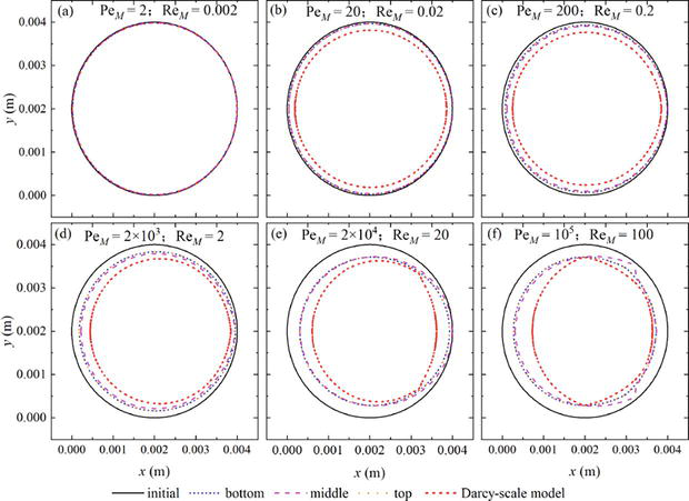
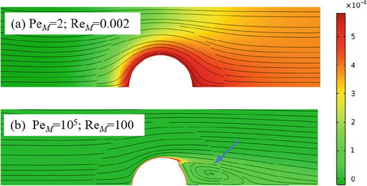
Three cross sections, namely the bottom, the middle and the top of the pillar obtained from DNS, are compared with Darcy-scale computations, after dissolution for ${10}^5$ s. As shown in Figure 4(a)–(c), the pillar first maintains circular cross sections and dissolves uniformly as observed at small ${\mathrm{Pe}}_M$ and ${Re}_M$. Then, the increases of ${\mathrm{Pe}}_M$ and ${Re}_M$ lead to the formation of a small cusp in the downstream of the pillar (see Figure 4(d)), where dissolution is slower than the upstream of the pillar because the liquid is much more saturated with dissolved minerals, which agrees well with the experimental observations reported [12, 42, 43]. However, when ${\mathrm{Pe}}_M$ reaches ${10}^5$ (and ${Re}_M$ reaches 100), the dissolution in the downstream of the pillar is flattened, as also observed in Ref. [44]. This is because that in the case of large ${Re}_M$, the back side of the pillar is within the region of steady-state inertia vortices that were observed to appear for a large enough Reynolds number, where the solute is well mixed rapidly. Comparing the streamlines as shown in Figure 5, we see that, unlike the attached flow in the case of small ${\mathrm{Pe}}_M$ and ${Re}_M$, there appear indeed steady vortices at the backside of the pillar when ${\mathrm{Pe}}_M$ and ${Re}_M$ are relatively large (indicated by the arrow in Figure 5 (b)).

Figure 4.

Geometry comparison between Darcy-scale model results and cross sections at three levels of the gypsum pillar after dissolution of ${10}^5$ s for different ${\mathrm{Pe}}_M$ and ${Re}_M$.

Figure 5.

Surface plotting of the mass fraction of ${\mathrm{Ca}}^{2+}$ and corresponding streamlines.

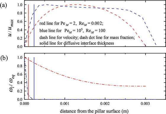
Regarding the accuracy of the Darcy-scale model, one can observe that when ${\mathrm{Pe}}_M$ and ${Re}_M$ are small, i.e., the mass transport process is dominated by diffusion and inertia and 3D effects are negligible, there is little difference between the size and circular shape of the three cross sections, which are remarkably well described by the Darcy model (see Figure 4(a)–(d)). However, when ${\mathrm{Pe}}_M\ge 2\times {10}^4$, even though the variation in the vertical direction is not profound, the Darcy-scale model failed to capture either the position or the shape of the dissolution interface and this discrepancy is increased dramatically from the condition with ${\mathrm{Pe}}_M=2\times {10}^4$ (${Re}_M=20$) to that with ${\mathrm{Pe}}_M={10}^5$ (${Re}_M=100$). This can be attributed to the fact that such conditions go beyond the assumption of small Reynolds number to develop the Darcy-scale model. In addition, as discussed in our previous work [1], to make sure the macro-scale model correctly reproduce the dissolution flux, the diffuse interface must not significantly affect the velocity and the mass fraction boundary layers, which means that the thickness of the diffuse interface (denoted as ${\delta }_D$), which can be defined by the zone where the porosity varies between the two limits, must be much smaller than the thicknesses of the velocity boundary layer $\left({\delta }_v\right)$ and the mass fraction boundary layer $\left({\delta }_{\omega }\right)$. From the results presented in Figure 6, one sees that this is indeed the case for diffusion dominated case, where we have ${\delta }_D\approx 0.0001$ m, ${\delta }_v\approx 0.0015$ m and ${\delta }_{\omega }\approx 0.003$ m, giving ${\delta }_D\ll {\delta }_v,{\delta }_{\omega }$. However, in the convection dominated case (see Figure 6), such a hypothesis breaks down, where the three lengths are comparable, i.e., ${\delta }_D\approx {\delta }_{\omega }\approx 0.0002$ m and ${\delta }_v\approx 0.0005$ m. The above results demonstrate that there is an upper limit of the applicability range of the Dary-scale model in terms of Péclet and Reynolds numbers, i.e., $\mathcal{O}\left({10}^3\right)$ and $\mathcal{O}\left(1\right)$, respectively, for the case considered here.

Figure 6.

Comparison of the velocity and mass fraction boundary layer thickness with that of the diffusive interface.

5. Conclusions

In this chapter, the upscaling of a mass transport problem involving a nonlinear heterogeneous reaction typical of dissolution problems has been carried out using a first-order Taylor’s expansion for the reaction rate when developing the equations for the concentration deviation. A full model including all couplings and the interface velocity has been obtained, and the closure problems providing the effective properties have been presented. To validate the Darcy-scale model, we have investigated the case of the dissolution of a cylindrical pillar located in a Hele-Shaw structure. In principle, the resulting pillar shape during the dissolution process becomes three dimensional. However, the shape remains nearly cylindrical for low Péclet and Reynolds numbers. It was found that a Darcy-Brinkman formulation with a no-slip condition on the pillar surface and the same dispersion equation managed to reproduce the pillar surface evolution up to relatively large Péclet and Reynolds numbers.

Additional information

Parts of this chapter were previously published in the doctoral thesis by the same author: Jianwei Guo. Numerical modelling of the dissolution of karstic cavities. 2015. Institut National Polytechnique de Toulouse. Available from: http://ethesis.inp-toulouse.fr/archive/00003105/.

Thanks

The author expresses her thanks to the financial supports from the National Natural Science Foundation of China (Grant 12102371), the Natural Science Foundation of Sichuan Province, China (Grant 2022NSFSC1932) and the Fundamental Research Funds for the Central Universities (Grant 2682022KJ049).

References

1.Guo J, Laouafa F, Quintard M. A theoretical and numerical framework for modeling gypsum cavity dissolution. International Journal for Numerical and Analytical Methods in Geomechanics. 2016;40:1662-1689
2.Cooper A. Halite karst geohazards (natural and man-made) in the United Kingdom. Environmental Geology. 2002;42(5):505-512
3.Hao Y, Smith M, Carroll S. Multiscale modeling of CO2-induced carbonate dissolution: From core to meter scale. International Journal of Greenhouse Gas Control. 2019;88:272-289
4.Li Q, Lin Z, Cai WH, Chen C-Y, Meiburg E. Dissolution-driven convection of low solubility fluids in porous media. International Journal of Heat and Mass Transfer. 2023;217:124624
5.Golfier F, Zarcone C, Bazin B, Lenormand R, Lasseux D, Quintard M. On the ability of a Darcy-scale model to capture wormhole formation during the dissolution of a porous medium. Journal of Fluid Mechanics. 2002;457:213-254
6.Kalia N, Balakotaiah V. Effect of medium heterogeneities on reactive dissolution of carbonates. Chemical Engineering Science. 2009;64(2):376-390
7.Liu P, Yan X, Yao J, Sun S. Modeling and analysis of the acidizing process in carbonate rocks using a two-phase thermal-hydrologic-chemical coupled model. Chemical Engineering Science. 2019;207:215-234
8.Panga MKR, Ziauddin M, Balakotaiah V. Two-scale continuum model for simulation of wormholes in carbonate acidization. AICHE Journal. 2005;51(12):3231-3248
9.Li X, Yang X. Effects of physicochemical properties and structural heterogeneity on mineral precipitation and dissolution in saturated porous media. Applied Geochemistry. 2022;146:105474
10.Békri S, Thovert JF, Adler PM. Dissolution of porous media. Chemical Engineering Science. 1995;50:2765-2791
11.Luo H, Quintard M, Debenest G, Laouafa F. Properties of a diffuse interface model based on a porous medium theory for solid-liquid dissolution problems. Computational Geosciences. 2012;16(4):913-932
12.Soulaine C, Roman S, Kovscek A, Tchelepi HA. Mineral dissolution and wormholing from a pore-scale perspective. Journal of Fluid Mechanics. 2017;827:457-483
13.Soulaine C, Roman S, Kovscek A, Tchelepi HA. Pore-scale modelling of multiphase reactive flow: Application to mineral dissolution with production of CO2. Journal of Fluid Mechanics. 2018;855:616-645
14.Starchenko V, Marra CJ, Ladd AJC. Three-dimensional simulations of fracture dissolution. Journal of Geophysical Research Solid Earth. 2016;121(9):6421-6444
15.Olsson E, Kreiss G. A conservative level set method for two phase flow. Journal of Computational Physics. 2005;210(1):225-246
16.Olsson E, Kreiss G, Zahedi S. A conservative level set method for two phase flow II. Journal of Computational Physics. 2007;225:785-807
17.Li H, Wang F, Wang Y, Yuan Y, Feng G, Tian H, et al. Phase-field modeling of coupled reactive transport and pore structure evolution due to mineral dissolution in porous media. Journal of Hydrology. 2023;619:129363
18.Békri S, Renard S, Delprat-Jannaud F. Pore to core scale simulation of the mass transfer with mineral reaction in porous media. Oil & Gas Science and Technology–Revue d’IFP Energies nouvelles. 2015;70:681-693
19.Varloteaux C, Békri S, Adler PM. Pore network modelling to determine the transport properties in presence of a reactive fluid: From pore to reservoir scale. Advances in Water Resources. 2013;53:87-100
20.Vignoles GL, Aspa Y, Quintard M. Modelling of carbon-carbon composite ablation in rocket nozzles. Composites Science and Technology. 2010;70(9):1303-1311
21.Taylor G. Dispersion of soluble matter in solvent flowing slowly through a tube. Proceedings of the Royal Society of London. Series A. Mathematical and Physical Sciences. 1953;219(1137):186-203
22.Taylor G. The dispersion of matter in turbulent flow through a pipe. Proceedings of the Royal Society of London. Series A. Mathematical and Physical Sciences. 1954;223(1155):446-468
23.Aris R. On the dispersion of a solute in a fluid flowing through a tube. Proceedings of the Royal Society of London. Series A. Mathematical and Physical Sciences. 1956;235(1200):67-77
24.Brenner H, Stewartson K. Dispersion resulting from flow through spatially periodic porous media. Philosophical Transactions of the Royal Society of London. Series A, Mathematical and Physical Sciences. 1980;297(1430):81-133
25.Eidsath A, Carbonell RG, Whitaker S, Herrmann LR. Dispersion in pulsed systems-III: Comparison between theory and experiments for packed beds. Chemical Engineering Science. 1983;38(11):1803-1816
26.Mei CC. Method of homogenization applied to dispersion in porous media. Transport in Porous Media. 1992;9(3):261-274
27.Bousquet-Melou P, Neculae A, Goyeau B, Quintard M. Averaged solute transport during solidification of a binary mixture: Active dispersion in dendritic structures. Metallurgical & Materials Transactions B. 2002;33(3):365-376
28.Coutelieris FA, Kainourgiakis ME, Stubos AK, Kikkinides ES, Yortsos YC. Multiphase mass transport with partitioning and inter-phase transport in porous media. Chemical Engineering Science. 2006;61(14):4650-4661
29.Guo J, Quintard M, Laouafa F. Dispersion in porous media with heterogeneous nonlinear reactions. Transport in Porous Media. 2015;109(3):541-570
30.Quintard M, Whitaker S. Convection, dispersion, and interfacial transport of contaminants: Homogeneous porous media. Advances in Water Resources. 1994;17:221-239
31.Whitaker S. The Method of Volume Averaging. Dordrecht, The Netherlands: Kluwer Academic Publishers; 1999
32.Cushman J, Ginn TR. Nonlocal dispersion in media with continuously evolving scales of heterogeneity. Transport in Porous Media. 1993;13:123-138
33.Dagan G. Flow and Transport in Porous Formations. Berlin-Heidelberg: Springer; 1989
34.Brenner H. Dispersion resulting from flow through spatially periodic porous media. Philosophical Transactions of the Royal Society of London. 1980;297:81-133
35.Shapiro M, Brenner H. Dispersion of a chemically reactive solute in a spatially periodic model of a porous medium. Chemical Engineering Science. 1988;43:551-571
36.Bensoussan A, Lions JL, Papanicolau G. Asymptotic Analysis for Periodic Structures. Amsterdam: North-Holland Publishing Company; 1978
37.Soulaine C, Debenest G, Quintard M. Upscaling multi-component two-phase flow in porous media with partitioning coefficient. Chemical Engineering Science. 2011;66:6180-6192
38.Valdés-Parada FJ, Aguilar-Madera CG, J. Álvarez-Ramírez on diffusion, dispersion and reaction in porous media. Chemical Engineering Science. 2011;66(10):2177-2190
39.Wood BD, Radakovich K, Golfier F. Effective reaction at a fluid-solid interface: Applications to biotransformation in porous media. Advances in Water Resources. 2007;30:1630-1647
40.Luo H, Laouafa F, Guo J, Quintard M. Numerical modeling of three-phase dissolution of underground cavities using a diffuse interface model. International Journal for Numerical and Analytical Methods in Geomechanics. 2014;38:1600-1616
41.Guo J, Laouafa F, Quintard M. On 2d approximations for dissolution problems in hele-Shaw cells. Science China-Physics, Mechanics and Astronomy. 2023;66:234711
42.Dutka F, Starchenko V, Osselin F, Magni S, Szymczak P, Ladd AJC. Time-dependent shapes of a dissolving mineral grain: Comparisons of simulations with microfluidic experiments. Chemical Geology. 2020;540:119459
43.Tan Q, Kang Y, You L, Peng H, Chen Q. Pore-scale investigation on mineral dissolution and evolution in hydrological properties of complex porous media with binary minerals. Chemical Geology. 2023;616:121247
44.Huang JM, Moore MNJ, Ristroph L. Shape dynamics and scaling laws for a body dissolving in fluid flow. Journal of Fluid Mechanics. 2015;765:R3
Written By
Jianwei Guo
Submitted: 22 August 2023Reviewed: 11 September 2023Published: 27 November 2023