The Paradigm of Complex Probability and Quantum Mechanics: The Quantum Harmonic Oscillator with Gaussian Initial Condition – The Momentum Wavefunction and the Wavefunction Entropies

Abstract

The system of probability axioms of Andrey Nikolaevich Kolmogorov put forward in 1933 can be developed to encompass the set of imaginary numbers after adding to his established five axioms a supplementary three axioms. Therefore, any probabilistic phenomenon can thus be performed in what is now the set of complex probabilities $\mathcal{C}$ which is the sum of the real set of probabilities $\mathcal{R}$ and the complementary and associated and corresponding imaginary set of probabilities $\mathcal{M}$. The aim here is to compute the complex probabilities by taking into consideration additional novel imaginary dimensions to the phenomenon that occurs in the “real” laboratory. Hence, the corresponding probability in the entire probability set $\mathcal{C}=\mathcal{R}+\mathcal{M}$ is, whatever the random distribution of the input random variable considered in $\mathcal{R}$, permanently and constantly equal to 1. Thus, the result of the stochastic experiment in $\mathcal{C}$ can be foretold perfectly and completely. Subsequently, the consequence shows that luck and chance in $\mathcal{R}$ is substituted now by absolute determinism in $\mathcal{C}$. Accordingly, this is the consequence of the fact that the probability in $\mathcal{C}$ is got by subtracting from the degree of our knowledge of the random system the chaotic factor. Henceforth, I will apply to the established and well-known theory of quantum mechanics my innovative and original Complex Probability Paradigm (CPP) which will yield a completely deterministic expression of quantum theory in the universe of probabilities $\mathcal{C}=\mathcal{R}+\mathcal{M}$.

1. Introduction

Firstly, classical physics explains energy and matter only on a familiar to human experience scale, and that includes the astronomical bodies behavior such as the planets or the moon [1, 2, 3, 4, 5, 6, 7, 8, 9, 10, 11, 12, 13]. By contrast, quantum mechanics studies matter and its interactions with energy on the subatomic particles and atomic scales. Knowing that, classical physics is still adopted in much of modern technology and science. However, towards the end of the nineteenth century, it was found by scientists that classical physics could not explain numerous phenomena discovered in both the macro (large) and the micro (small) worlds. Hence, the theory of relativity and the theory of quantum mechanics were developed to resolve inconsistencies between classical theory and observed phenomena. Thus, this has led to these two major revolutions in physics that resulted to a shift in the original scientific paradigm. Therefore, physicists discovered the limitations of classical physics and developed the main concepts of the quantum theory that replaced it in the early decades of the twentieth century. They described these concepts in roughly the order in which they were first discovered.

Moreover, light behaves in some aspects like waves and in other aspects like particles. Matter which is the “stuff” of the universe is made up of particles such as protons, electrons, neutrons, and atoms and which show wavelike behavior also. Additionally, neon lights, like some light sources, exhibit only certain definite frequencies of light, which is a small set of distinct pure colors fixed by the atomic structure of neon. Quantum mechanics proves that light, along with all other forms of electromagnetic radiation, comes in photons that are discrete units, and calculates the spectral energies that correspond to pure colors, and it computes as well its light beams intensities. The smallest observable particle of the electromagnetic field is a single photon also called a quantum. Knowing that, we have never experimentally observed a partial photon. More broadly, many properties of objects, such as position, speed, and angular momentum, that appeared continuous in the zoomed-out view of classical mechanics, turn out to be quantized in the very tiny, zoomed-in scale of quantum mechanics as it was shown by quantum theory. Such elementary particle properties are necessary to take on one of a set of discrete and small allowable values. But since the gap between these discrete values is similarly small, then the discontinuities are only noticed at very tiny atomic scales.

Furthermore, many features of quantum mechanics can seem to be paradoxical and are counterintuitive because they describe behavior quite dissimilar to that seen at larger scales. The famous quantum physicist Richard Feynman describes quantum mechanics as a theory that deals with “nature as She is—absurd.” One major “paradox” is the apparent inconsistency between quantum mechanics and Newton’s laws and which can be clarified using the theorem of Ehrenfest. In his theorem, the latter proves that the obtained quantum mechanics average values (like position and momentum) obey and respect classical laws. However, the theorem of Ehrenfest is far from being capable of explaining all the observed counterintuitive phenomena of quantum weirdness, but rather is a mathematical expression of the principle of correspondence.

Moreover, the quantum-mechanical analog of the classical harmonic oscillator is the quantum harmonic oscillator. It is one of the most important model systems in quantum mechanics because an arbitrary smooth potential can generally be estimated as a harmonic potential at the neighborhood of a stable equilibrium point. Furthermore, since an exact, analytical solution is known, then it is one of the few quantum-mechanical systems for which this kind of solution is provided. Consequently, I will relate my complex probability paradigm (CPP) to this well-known and important problem in quantum mechanics in order to express it completely deterministically.

At the end, and to conclude, this research work is organized as follows: In Section 1, we will present the introduction, and then in Section 2 we will explain the advantages and the purpose of the present work. Afterward, in Section 3, we will explain and summarize the extended Kolmogorov’s axioms and hence present the original parameters and interpretation of the complex probability paradigm. Additionally, in Section 4, the new paradigm will be related to the quantum harmonic oscillators with Gaussian initial condition problem after applying CPP to the momentum wavefunction of the problem in this current second chapter, hence some corresponding simulations will be done, and afterward the characteristics of this stochastic distribution will be computed in the probabilities sets $\mathcal{R}$, $\mathcal{M}$, and $\mathcal{C}$. Furthermore, in Section 5, CPP will be used to extend and to verify the Quantum Uncertainty Principle in $\mathcal{R}$, $\mathcal{M}$, and $\mathcal{C}$. In addition, in Section 6, we will calculate and determine the position and the momentum wavefunctions entropies in $\mathcal{R}$, $\mathcal{M}$, and $\mathcal{C}$. Finally, we conclude the work by doing a comprehensive summary in Section 7 and then present the list of references cited in the current research work.

2. The purpose and the advantages of the current publication

Computing probabilities is all our work in the classical theory of probability [14, 15, 16, 17, 18, 19, 20, 21, 22, 23, 24, 25, 26, 27, 28, 29, 30, 31, 32, 33, 34, 35, 36]. Adding new dimensions to our stochastic experiment is the innovative idea in the current paradigm which will make the study absolutely deterministic. As a matter of fact, the theory of probability is a nondeterministic theory by essence that means that all the random events outcome is due to luck and chance. Hence, we make the study deterministic by adding new imaginary dimensions to the phenomenon occurring in the “real” laboratory which is $\mathcal{R}$, and therefore, a stochastic experiment will have a certain outcome in the complex probabilities set $\mathcal{C}$. It is of great significance that random systems become completely predictable since we will be perfectly knowledgeable to predict the outcome of all stochastic and chaotic phenomena that occur in nature like for example in all stochastic processes, in statistical mechanics, or in the well-established field of quantum mechanics. Consequently, the work that should be done is to add the contributions of $\mathcal{M}$ which is the set of imaginary probabilities to the set of real probabilities$\mathcal{R}$ that will make the random phenomenon in $\mathcal{C}=\mathcal{R}+\mathcal{M}$ completely deterministic. Since this paradigm is found to be fruitful, then a new theory in prognostic and stochastic sciences is established and this is to understand deterministically those events that used to be stochastic events in $\mathcal{R}$. This is what I coined by the term “The Complex Probability Paradigm” that was elaborated and initiated in my 23 previous papers.

To summarize, the advantages and the purposes of this current work and chapter are to:

1. Relate probability theory to the field of complex variables and analysis in mathematics and therefore to extend the theory of classical probability to the set of complex numbers. This task was elaborated and initiated in my 23 previous papers.

2. Apply the novel probability axioms and CPP paradigm to quantum mechanics, specifically to the quantum harmonic oscillators with Gaussian initial condition problem.

3. Demonstrate that any stochastic and random event and experiment can be expressed deterministically in the complex probabilities set$\mathcal{C}$.

4. Quantify both the chaos magnitude and the degree of our knowledge of the wavefunction momentum distribution and CPP in the sets $\mathcal{R}$, $\mathcal{M}$, and $\mathcal{C}$.

5. Represent graphically and illustrate the parameters and functions of the original paradigm related to this quantum mechanics problem.

6. Evaluate all the characteristics of the wavefunction momentum distribution.

7. Demonstrate that the classical concepts of stochastic system have a probability of occurring permanently equal to one in the complex set; consequently, no ignorance, no unpredictability, no stochasticity, no disorder, no randomness, no nondeterminism, and no chaos exist in:

   $$\mathcal{C}\left(\text{complex}\mathrm{set}\right)=\mathcal{R}\left(\text{real}\mathrm{set}\right)+\mathcal{M}\left(\text{imaginary}\mathrm{set}\right).$$E1

8. Verify and extend the Quantum Uncertainty Principle in $\mathcal{R}$to $\mathcal{M}$ and $\mathcal{C}$.

9. Calculate the problem entropies in $\mathcal{R}$, $\mathcal{M}$, and $\mathcal{C}$ and show that there is no disorder and no information loss or gain in CPP but conservation of information.

10. Prepare to apply the novel paradigm to other topics in stochastic processes, in statistical mechanics, and to the field of prognostics in science and engineering and quantum mechanics. This will be the task in my following research work and publications.

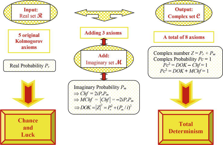
Compared with existing literature, the major contribution of the current research work is to apply the novel paradigm of CPP to quantum mechanics and to express it completely deterministically. And concerning some applications of the novel developed paradigm and as a future work, it can be applied to any nondeterministic phenomenon in quantum mechanics. The next figure displays the major purposes of the Complex Probability Paradigm (CPP) (Figure 1).

Figure 1.

The diagram of the Complex Probability Paradigm applied to Quantum Mechanics major purposes and goals.

3. The complex probability paradigm

3.1 The original Andrey Nikolaevich Kolmogorov system of axioms

The simplicity of Kolmogorov’s system of axioms may be surprising [14, 15, 16, 17, 18, 19, 20, 21, 22, 23, 24, 25, 26, 27, 28, 29, 30, 31, 32, 33, 34, 35, 36]. Let E be a collection of elements {E₁, E₂, …} called elementary events and let F be a set of subsets of E called random events [37, 38, 39, 40]. The five axioms for a finite set E are:

Axiom 1: F is a field of sets.

Axiom 2: F contains the set E.

Axiom 3: A non-negative real number P_rob(A), called the probability of A, is assigned to each set A in F. We have always 0 ≤ P_rob(A) ≤ 1.

Axiom 4: P_rob(E) equals 1.

Axiom 5: If A and B have no elements in common, the number assigned to their union is:

$$P_{\mathit{rob}}\left(A\cup B\right)=P_{\mathit{rob}}\left(A\right)+P_{\mathit{rob}}\left(B\right)$$E2

hence, we say that A and B are disjoint; otherwise, we have:

$$P_{\mathit{rob}}\left(A\cup B\right)=P_{\mathit{rob}}\left(A\right)+P_{\mathit{rob}}\left(B\right)-P_{\mathit{rob}}\left(A\cap B\right)$$E3

And we say also that: $P_{\mathit{rob}}\left(A\cap B\right)=P_{\mathit{rob}}\left(A\right)\times P_{\mathit{rob}}\left(B/A\right)=P_{\mathit{rob}}\left(B\right)\times P_{\mathit{rob}}\left(A/B\right)$ which is the conditional probability. If both A and B are independent then: $P_{\mathit{rob}}\left(A\cap B\right)=P_{\mathit{rob}}\left(A\right)\times P_{\mathit{rob}}\left(B\right)$.

Moreover, we can generalize and say that for N disjoint (mutually exclusive) events $A_1,A_2,\dots ,A_j,\dots ,A_N$ (for $1\le j\le N$), we have the following additivity rule:

$$P_{\mathit{rob}}\left(\bigcup _{j=1}^N{A}_j\right)=\sum _{j=1}^N{P}_{\mathit{rob}}\left(A_j\right)$$E4

And we say also that for N independent events $A_1,A_2,\dots ,A_j,\dots ,A_N$ (for $1\le j\le N$), we have the following product rule:

$$P_{\mathit{rob}}\left(\bigcap _{j=1}^N{A}_j\right)=\prod _{j=1}^N{P}_{\mathit{rob}}\left(A_j\right)$$E5

3.2 Adding the imaginary part $\mathcal{M}$

Now, we can add to this system of axioms an imaginary part such that:

Axiom 6: Let $P_m=i\times \left(1-P_r\right)$ be the probability of an associated complementary event in $\mathcal{M}$ (the imaginary part or universe) to the event A in $\mathcal{R}$ (the real part or universe). It follows that $P_r+P_m/i=1$ where i is the imaginary number with $i=\sqrt{-1}$ or $i^2=-1$.

Axiom 7: We construct the complex number or vector $Z=P_r+P_m=P_r+i\left(1-P_r\right)$ having a norm $\left|Z\right|$ such that:

$${\left|Z\right|}^2=P_r^2+{\left(P_m/i\right)}^2.$$E6

Axiom 8: Let Pc denote the probability of an event in the complex probability set and universe $\mathcal{C}$ where $\mathcal{C}=\mathcal{R}+\mathcal{M}$. We say that Pc is the probability of an event A in $\mathcal{R}$ with its associated and complementary event in $\mathcal{M}$ such that:

$${\mathit{Pc}}^2={\left(P_r+P_m/i\right)}^2={\left|Z\right|}^2-2{\mathit{iP}}_r{P}_m\text{and is always equal to}1.$$E7

We can see that by taking into consideration the set of imaginary probabilities we added three new and original axioms and consequently the system of axioms defined by Kolmogorov was hence expanded to encompass the set of imaginary numbers and realm [41, 42, 43, 44, 45, 46, 47, 48, 49, 50, 51, 52, 53, 54, 55, 56, 57, 58, 59, 60, 61, 62, 63, 64, 65, 66, 67, 68].

3.3 A concise interpretation of the original CPP paradigm

To conclude and to summarize, we state that our degree of our certain knowledge is undesirably incomplete and imperfect and thus unsatisfactory in the real probability universe $\mathcal{R}$. Hence, we extend our study to the set of complex numbers $\mathcal{C}$ which includes the contributions of both the set of real probabilities which is $\mathcal{R}$ and the set of complementary imaginary probabilities which is$\mathcal{M}$. Consequently, this will result to a perfect and absolute degree of our knowledge in the probability universe$\mathcal{C}$ = $\mathcal{R}$ + $\mathcal{M}$ because Pc = 1 continuously. In fact, the study in the complex universe $\mathcal{C}$ leads to a certain prediction of any stochastic and random event and experiment since in $\mathcal{C}$ we subtract and eliminate the measured chaotic factor from our computed degree of our knowledge. This will result to a probability permanently equal to 1 in the universe $\mathcal{C}$ as it is shown in the following equation deduced from CPP: ${\mathit{Pc}}^2=\mathit{DOK}-\mathit{Chf}=\mathit{DOK}+\mathit{\text{MChf}}=1=\mathit{Pc}$. Many numerous discrete and continuous probability distributions were illustrated in my 23 previous research works and that confirm this hypothesis and original paradigm [14, 15, 16, 17, 18, 19, 20, 21, 22, 23, 24, 25, 26, 27, 28, 29, 30, 31, 32, 33, 34, 35, 36]. The Extended Kolmogorov Axioms (EKA for short) or the Complex Probability Paradigm (CPP for short) can be summarized and shown in the next illustration (Figure 2):

Figure 2.

The EKA or the CPP diagram.

4. The quantum harmonic oscillator with Gaussian initial condition and the complex probability paradigm (CPP) parameters: The momentum wavefunction and CPP

In this section, we will relate and link quantum mechanics to the complex probability paradigm with all its parameters by applying it to the quantum harmonic oscillators with Gaussian initial condition and this by using the four CPP concepts which are: the real probability $P_r$ in the real probability set $\mathcal{R}$, the imaginary probability $P_m$ in the imaginary probability set $\mathcal{M}$, the complex random vector or number $Z$ in the complex probability set $\mathcal{C}=\mathcal{R}+\mathcal{M}$, and the deterministic real probability $\mathit{Pc}$ also in the probability set $\mathcal{C}$ [1, 2, 3, 4, 5, 6, 7, 8, 9, 10, 11, 12, 13, 14, 15, 16, 17, 18, 19, 20, 21, 22, 23, 24, 25, 26, 27, 28, 29, 30, 31, 32, 33, 34, 35, 36, 69, 70, 71, 72, 73, 74, 75, 76, 77, 78, 79, 80].

4.1 The momentum wavefunction probability distribution and CPP

The probability momentum density for the quantum harmonic oscillators with Gaussian initial condition problem is derived from the wavefunction as $f\left(p\right)={\left|\varphi \left(p,t\right)\right|}^2$. Through integration over the propagator, we can solve for the full time-dependent solution. After many cancelations, and as with position, the wavefunction momentum probability density function (PDF) reduces to and is given by [1, 2, 3]:

$$f\left(p\right)={\left|\varphi \left(p,t\right)\right|}^2=\mathbb{N}\left(-{\mathit{mx}}_{0}wsin\left(\mathit{wt}\right),\sqrt{\frac{\mathrm{\hslash }m\mathrm{\Omega }}{2}\left({cos}^2\left(\mathit{wt}\right)+\frac{w^2}{{\mathrm{\Omega }}^2}{sin}^2\left(\mathit{wt}\right)\right)}\right)$$E8

Where the mean of the normal distribution $\mathbb{N}\left({\mu }_P,{\sigma }_P\right)$ is = ${\mu }_p=-{\mathit{mx}}_{0}wsin\left(\mathit{wt}\right)$.

and the standard deviation of this normal distribution is = ${\sigma }_p=\sqrt{\frac{\mathrm{\hslash }m\mathrm{\Omega }}{2}\left({cos}^2\left(\mathit{wt}\right)+\frac{w^2}{{\mathrm{\Omega }}^2}{sin}^2\left(\mathit{wt}\right)\right)}$and $\mathrm{\hslash }=\frac{h}{2\pi }$ is the reduced Planck constant, and $w$ is the characteristic angular frequency, and with $\mathrm{\Omega }$ describing the width of the initial state but need not be the same as $w$. Knowing that, we have taken in this study $\mathrm{\Omega }=n\times w$ where $n$ is a simple multiplier and can be equal to ½, or 1, or 2, or 30, or 100, or 500, etc., as it will be shown afterward in the simulations section. Also, in a quantum harmonic oscillator of characteristic angular frequency $w$, we place a state that is offset from the bottom of the potential by some displacement $x_0$ as it is shown in the equation [1, 2, 3]:

$$\mathrm{\Psi }\left(x,t=0\right)={\left(\frac{m\mathrm{\Omega }}{\pi \mathrm{\hslash }}\right)}^{1/4}exp\left(-\frac{m\mathrm{\Omega }{\left(x-x_0\right)}^2}{2\mathrm{\hslash }}\right)$$E9

Therefore, the wavefunction momentum cumulative probability distribution function (CDF) which is equal to $P_r\left(T\right)$ in $\mathcal{R}$ is:

$$\begin{array}{l}{P}_r\left(T\right)=F\left(t_j\right)=P_{\mathit{rob}}\left(T\le t_j\right)=\underset{0}{\overset{t_j}{\int }}{\left|\varphi \left(p,t\right)\right|}^2\mathit{dt}\\ =\underset{0}{\overset{t_j}{\int }}\mathbb{N}\left(-{\mathit{mx}}_{0}wsin\left(\mathit{wt}\right),\sqrt{\frac{\mathrm{\hslash }m\mathrm{\Omega }}{2}\left({cos}^2\left(\mathit{wt}\right)+\frac{w^2}{{\mathrm{\Omega }}^2}{sin}^2\left(\mathit{wt}\right)\right)}\right)\mathit{dt}\end{array}$$E10

And the real complementary probability to $P_r\left(T\right)$ in $\mathcal{R}$ which is $P_m\left(T\right)/i$ is:

$$\begin{array}{l}{P}_m\left(T\right)/i=1-P_r\left(T\right)=1-F\left(t_j\right)=1-P_{\mathit{rob}}\left(T\le t_j\right)=P_{\mathit{rob}}\left(T>t_j\right)=1-\underset{0}{\overset{t_j}{\int }}{\left|\varphi \left(p,t\right)\right|}^2\mathit{dt}\\ =\underset{t_j}{\overset{+\infty }{\int }}{\left|\varphi \left(p,t\right)\right|}^2\mathit{dt}\\ =1-\underset{0}{\overset{t_j}{\int }}\mathbb{N}\left(-{\mathit{mx}}_{0}wsin\left(\mathit{wt}\right),\sqrt{\frac{\mathrm{\hslash }m\mathrm{\Omega }}{2}\left({cos}^2\left(\mathit{wt}\right)+\frac{w^2}{{\mathrm{\Omega }}^2}{sin}^2\left(\mathit{wt}\right)\right)}\right)\mathit{dt}\\ =\underset{t_j}{\overset{+\infty }{\int }}\mathbb{N}\left(-{\mathit{mx}}_{0}wsin\left(\mathit{wt}\right),\sqrt{\frac{\mathrm{\hslash }m\mathrm{\Omega }}{2}\left({cos}^2\left(\mathit{wt}\right)+\frac{w^2}{{\mathrm{\Omega }}^2}{sin}^2\left(\mathit{wt}\right)\right)}\right)\mathit{dt}\end{array}$$E11

Consequently, the imaginary complementary probability to $P_r\left(T\right)$ in $\mathcal{M}$ which is $P_m\left(T\right)$ is:

$$\begin{array}{l}{P}_m\left(T\right)=i\left[1-P_r\left(T\right)\right]=i\left[1-F\left(t_j\right)\right]=i\left[1-P_{\mathit{rob}}\left(T\le t_j\right)\right]={\mathit{iP}}_{\mathit{rob}}\left(T>t_j\right)\\ =i\left[1-\underset{0}{\overset{t_j}{\int }}{\left|\varphi \left(p,t\right)\right|}^2\mathit{dt}\right]=i\underset{t_j}{\overset{+\infty }{\int }}{\left|\varphi \left(p,t\right)\right|}^2\mathit{dt}\\ =i\left[1-\underset{0}{\overset{t_j}{\int }}\mathbb{N}\left(-{\mathit{mx}}_{0}wsin\left(\mathit{wt}\right),\sqrt{\frac{\mathrm{\hslash }m\mathrm{\Omega }}{2}\left({cos}^2\left(\mathit{wt}\right)+\frac{w^2}{{\mathrm{\Omega }}^2}{sin}^2\left(\mathit{wt}\right)\right)}\right)\mathit{dt}\right]\\ =i\underset{t_j}{\overset{+\infty }{\int }}\mathbb{N}\left(-{\mathit{mx}}_{0}wsin\left(\mathit{wt}\right),\sqrt{\frac{\mathrm{\hslash }m\mathrm{\Omega }}{2}\left({cos}^2\left(\mathit{wt}\right)+\frac{w^2}{{\mathrm{\Omega }}^2}{sin}^2\left(\mathit{wt}\right)\right)}\right)\mathit{dt}\end{array}$$E12

Furthermore, the complex random number or vector in $\mathcal{C}=\mathcal{R}+\mathcal{M}$ which is $Z\left(T\right)$ is:

$$\begin{array}{l}Z\left(T\right)=P_r\left(T\right)+P_m\left(T\right)=P_r\left(T\right)+i\left[1-P_r\left(T\right)\right]=F\left(t_j\right)+i\left[1-F\left(t_j\right)\right]\\ =P_{\mathit{rob}}\left(T\le t_j\right)+i\left[1-P_{\mathit{rob}}\left(T\le t_j\right)\right]=P_{\mathit{rob}}\left(T\le t_j\right)+{\mathit{iP}}_{\mathit{rob}}\left(T>t_j\right)\\ =\underset{0}{\overset{t_j}{\int }}{\left|\varphi \left(p,t\right)\right|}^2\mathit{dt}+i\left[1-\underset{0}{\overset{t_j}{\int }}{\left|\varphi \left(p,t\right)\right|}^2\mathit{dt}\right]=\underset{0}{\overset{t_j}{\int }}{\left|\varphi \left(p,t\right)\right|}^2\mathit{dt}+i\underset{t_j}{\overset{+\infty }{\int }}{\left|\varphi \left(p,t\right)\right|}^2\mathit{dt}\end{array}$$

$$\begin{array}{l}=\left[\underset{0}{\overset{t_j}{\int }}\mathbb{N}\left(-{\mathit{mx}}_{0}wsin\left(\mathit{wt}\right),\sqrt{\frac{\mathrm{\hslash }m\mathrm{\Omega }}{2}\left({cos}^2\left(\mathit{wt}\right)+\frac{w^2}{{\mathrm{\Omega }}^2}{sin}^2\left(\mathit{wt}\right)\right)}\right)\mathit{dt}\right]\\ +i\left[1-\underset{0}{\overset{t_j}{\int }}\mathbb{N}\left(-{\mathit{mx}}_{0}wsin\left(\mathit{wt}\right),\sqrt{\frac{\mathrm{\hslash }m\mathrm{\Omega }}{2}\left({cos}^2\left(\mathit{wt}\right)+\frac{w^2}{{\mathrm{\Omega }}^2}{sin}^2\left(\mathit{wt}\right)\right)}\right)\mathit{dt}\right]\\ =\left[\underset{0}{\overset{t_j}{\int }}\mathbb{N}\left(-{\mathit{mx}}_{0}wsin\left(\mathit{wt}\right),\sqrt{\frac{\mathrm{\hslash }m\mathrm{\Omega }}{2}\left({cos}^2\left(\mathit{wt}\right)+\frac{w^2}{{\mathrm{\Omega }}^2}{sin}^2\left(\mathit{wt}\right)\right)}\right)\mathit{dt}\right]\\ +i\left[\underset{t_j}{\overset{+\infty }{\int }}\mathbb{N}\left(-{\mathit{mx}}_{0}wsin\left(\mathit{wt}\right),\sqrt{\frac{\mathrm{\hslash }m\mathrm{\Omega }}{2}\left({cos}^2\left(\mathit{wt}\right)+\frac{w^2}{{\mathrm{\Omega }}^2}{sin}^2\left(\mathit{wt}\right)\right)}\right)\mathit{dt}\right]\end{array}$$E13

Additionally, the degree of our knowledge which is $\mathit{DOK}\left(T\right)$ is:

$$\begin{array}{rcl}\mathit{DOK}\left(T\right)& =& {\left[P_r\left(T\right)\right]}^2+{\left[P_m\left(T\right)/i\right]}^2={\left[P_r\left(T\right)\right]}^2+{\left[1-P_r\left(T\right)\right]}^2={\left[F\left(t_j\right)\right]}^2+{\left[1-F\left(t_j\right)\right]}^2\\ & =& {\left[P_{\mathit{rob}}\left(T\le t_j\right)\right]}^2+{\left[1-P_{\mathit{rob}}\left(T\le t_j\right)\right]}^2={\left[P_{\mathit{rob}}\left(T\le t_j\right)\right]}^2+{\left[P_{\mathit{rob}}\left(T>t_j\right)\right]}^2\\ & =& {\left[\underset{0}{\overset{t_j}{\int }}{\left|\varphi \left(p,t\right)\right|}^2\mathit{dt}\right]}^2+{\left[1-\underset{0}{\overset{t_j}{\int }}{\left|\varphi \left(p,t\right)\right|}^2\mathit{dt}\right]}^2\\ & =& {\left[\underset{0}{\overset{t_j}{\int }}{\left|\varphi \left(p,t\right)\right|}^2\mathit{dt}\right]}^2+{\left[\underset{t_j}{\overset{+\infty }{\int }}{\left|\varphi \left(p,t\right)\right|}^2\mathit{dt}\right]}^2\end{array}$$

$$\begin{array}{l}={\left[\underset{0}{\overset{t_j}{\int }}\mathbb{N}\left(-{\mathit{mx}}_{0}wsin\left(\mathit{wt}\right),\sqrt{\frac{\mathrm{\hslash }m\mathrm{\Omega }}{2}\left({cos}^2\left(\mathit{wt}\right)+\frac{w^2}{{\mathrm{\Omega }}^2}{sin}^2\left(\mathit{wt}\right)\right)}\right)\mathit{dt}\right]}^2\\ +{\left[1-\underset{0}{\overset{t_j}{\int }}\mathbb{N}\left(-{\mathit{mx}}_{0}wsin\left(\mathit{wt}\right),\sqrt{\frac{\mathrm{\hslash }m\mathrm{\Omega }}{2}\left({cos}^2\left(\mathit{wt}\right)+\frac{w^2}{{\mathrm{\Omega }}^2}{sin}^2\left(\mathit{wt}\right)\right)}\right)\mathit{dt}\right]}^2\\ ={\left[\underset{0}{\overset{t_j}{\int }}\mathbb{N}\left(-{\mathit{mx}}_{0}wsin\left(\mathit{wt}\right),\sqrt{\frac{\mathrm{\hslash }m\mathrm{\Omega }}{2}\left({cos}^2\left(\mathit{wt}\right)+\frac{w^2}{{\mathrm{\Omega }}^2}{sin}^2\left(\mathit{wt}\right)\right)}\right)\mathit{dt}\right]}^2\\ +{\left[\underset{t_j}{\overset{+\infty }{\int }}\mathbb{N}\left(-{\mathit{mx}}_{0}wsin\left(\mathit{wt}\right),\sqrt{\frac{\mathrm{\hslash }m\mathrm{\Omega }}{2}\left({cos}^2\left(\mathit{wt}\right)+\frac{w^2}{{\mathrm{\Omega }}^2}{sin}^2\left(\mathit{wt}\right)\right)}\right)\mathit{dt}\right]}^2\end{array}$$E14

Moreover, the chaotic factor which is $\mathit{Chf}\left(T\right)$ is:

$$\begin{array}{rcl}\mathit{Chf}\left(T\right)& =& 2{\mathit{iP}}_r\left(T\right)P_m\left(T\right)=2{\mathit{iP}}_r\left(T\right)\times i\left[1-P_r\left(T\right)\right]=-2P_r\left(T\right)\left[1-P_r\left(T\right)\right]\\ & & =-2F\left(t_j\right)\left[1-F\left(t_j\right)\right]\\ & =& -2P_{\mathit{rob}}\left(T\le t_j\right)\left[1-P_{\mathit{rob}}\left(T\le t_j\right)\right]=-2P_{\mathit{rob}}\left(T\le t_j\right)P_{\mathit{rob}}\left(T>t_j\right)\\ & =& -2\left[\underset{0}{\overset{t_j}{\int }}{\left|\varphi \left(p,t\right)\right|}^2\mathit{dt}\right]\times \left[1-\underset{0}{\overset{t_j}{\int }}{\left|\varphi \left(p,t\right)\right|}^2\mathit{dt}\right]\\ & =& -2\left[\underset{0}{\overset{t_j}{\int }}{\left|\varphi \left(p,t\right)\right|}^2\mathit{dt}\right]\times \left[\underset{t_j}{\overset{+\infty }{\int }}{\left|\varphi \left(p,t\right)\right|}^2\mathit{dt}\right]\\ & =& -2\left[\underset{0}{\overset{t_j}{\int }}\mathbb{N}\left(-{\mathit{mx}}_{0}wsin\left(\mathit{wt}\right),\sqrt{\frac{\mathrm{\hslash }m\mathrm{\Omega }}{2}\left({cos}^2\left(\mathit{wt}\right)+\frac{w^2}{{\mathrm{\Omega }}^2}{sin}^2\left(\mathit{wt}\right)\right)}\right)\mathit{dt}\right]\\ & & \times [1-\underset{0}{\overset{t_j}{\int }}\mathbb{N}\left(-{\mathit{mx}}_{0}wsin\left(\mathit{wt}\right),\sqrt{\frac{\mathrm{\hslash }m\mathrm{\Omega }}{2}\left({cos}^2\left(\mathit{wt}\right)+\frac{w^2}{{\mathrm{\Omega }}^2}{sin}^2\left(\mathit{wt}\right)\right)}\right)\mathit{dt}]\\ & =& -2\left[\underset{0}{\overset{t_j}{\int }}\mathbb{N}\left(-{\mathit{mx}}_{0}wsin\left(\mathit{wt}\right),\sqrt{\frac{\mathrm{\hslash }m\mathrm{\Omega }}{2}\left({cos}^2\left(\mathit{wt}\right)+\frac{w^2}{{\mathrm{\Omega }}^2}{sin}^2\left(\mathit{wt}\right)\right)}\right)\mathit{dt}\right]\\ & & \times \left[\underset{t_j}{\overset{+\infty }{\int }}\mathbb{N}\left(-{\mathit{mx}}_{0}wsin\left(\mathit{wt}\right),\sqrt{\frac{\mathrm{\hslash }m\mathrm{\Omega }}{2}\left({cos}^2\left(\mathit{wt}\right)+\frac{w^2}{{\mathrm{\Omega }}^2}{sin}^2\left(\mathit{wt}\right)\right)}\right)\mathit{dt}\right]\end{array}$$E15

In addition, the magnitude of the chaotic factor which is $\mathit{\text{MChf}}\left(T\right)$ is:

$$\begin{array}{rcl}\mathit{\text{MChf}}\left(T\right)& =& \left|\mathit{Chf}\left(T\right)\right|=-2{\mathit{iP}}_r\left(T\right)P_m\left(T\right)=-2{\mathit{iP}}_r\left(T\right)\times i\left[1-P_r\left(T\right)\right]=2P_r\left(T\right)\left[1-P_r\left(T\right)\right]\\ & & =2F\left(t_j\right)\left[1-F\left(t_j\right)\right]\\ & =& 2P_{\mathit{rob}}\left(T\le t_j\right)\left[1-P_{\mathit{rob}}\left(T\le t_j\right)\right]=2P_{\mathit{rob}}\left(T\le t_j\right)P_{\mathit{rob}}\left(T>t_j\right)\\ & =& 2\left[\underset{0}{\overset{t_j}{\int }}{\left|\varphi \left(p,t\right)\right|}^2\mathit{dt}\right]\times \left[1-\underset{0}{\overset{t_j}{\int }}{\left|\varphi \left(p,t\right)\right|}^2\mathit{dt}\right]\\ & =& 2\left[\underset{0}{\overset{t_j}{\int }}{\left|\varphi \left(p,t\right)\right|}^2\mathit{dt}\right]\times \left[\underset{t_j}{\overset{+\infty }{\int }}{\left|\varphi \left(p,t\right)\right|}^2\mathit{dt}\right]\\ & =& 2\left[\underset{0}{\overset{t_j}{\int }}\mathbb{N}\left(-{\mathit{mx}}_{0}wsin\left(\mathit{wt}\right),\sqrt{\frac{\mathrm{\hslash }m\mathrm{\Omega }}{2}\left({cos}^2\left(\mathit{wt}\right)+\frac{w^2}{{\mathrm{\Omega }}^2}{sin}^2\left(\mathit{wt}\right)\right)}\right)\mathit{dt}\right]\\ & \times & \left[1-\underset{0}{\overset{t_j}{\int }}\mathbb{N}\left(-{\mathit{mx}}_{0}wsin\left(\mathit{wt}\right),\sqrt{\frac{\mathrm{\hslash }m\mathrm{\Omega }}{2}\left({cos}^2\left(\mathit{wt}\right)+\frac{w^2}{{\mathrm{\Omega }}^2}{sin}^2\left(\mathit{wt}\right)\right)}\right)\mathit{dt}\right]\\ & =& 2\left[\underset{0}{\overset{t_j}{\int }}\mathbb{N}\left(-{\mathit{mx}}_{0}wsin\left(\mathit{wt}\right),\sqrt{\frac{\mathrm{\hslash }m\mathrm{\Omega }}{2}\left({cos}^2\left(\mathit{wt}\right)+\frac{w^2}{{\mathrm{\Omega }}^2}{sin}^2\left(\mathit{wt}\right)\right)}\right)\mathit{dt}\right]\\ & \times & \left[\underset{t_j}{\overset{+\infty }{\int }}\mathbb{N}\left(-{\mathit{mx}}_{0}wsin\left(\mathit{wt}\right),\sqrt{\frac{\mathrm{\hslash }m\mathrm{\Omega }}{2}\left({cos}^2\left(\mathit{wt}\right)+\frac{w^2}{{\mathrm{\Omega }}^2}{sin}^2\left(\mathit{wt}\right)\right)}\right)\mathit{dt}\right]\end{array}$$E16

Finally, the real probability in the complex probability universe $\mathcal{C}=\mathcal{R}+\mathcal{M}$ which is $\mathit{Pc}\left(T\right)$ is:

$$\begin{array}{rcl}{\mathit{Pc}}^2\left(T\right)& =& {\left\{\left[P_r\left(T\right)\right]+\left[P_m\left(T\right)/i\right]\right\}}^2={\left\{\left[P_r\left(T\right)\right]+\left[1-P_r\left(T\right)\right]\right\}}^2\\ & =& {\left\{\left[F\left(t_j\right)\right]+\left[1-F\left(t_j\right)\right]\right\}}^2={\left\{P_{\mathit{rob}}\left(T\le t_j\right)+\left[1-P_{\mathit{rob}}\left(T\le t_j\right)\right]\right\}}^2\\ & =& {\left\{P_{\mathit{rob}}\left(T\le t_j\right)+P_{\mathit{rob}}\left(T>t_j\right)\right\}}^2\\ & =& {\left\{\underset{0}{\overset{t_j}{\int }}{\left|\varphi \left(p,t\right)\right|}^2\mathit{dt}+\left[1-\underset{0}{\overset{t_j}{\int }}{\left|\varphi \left(p,t\right)\right|}^2\mathit{dt}\right]\right\}}^2\\ & =& {\left\{\underset{0}{\overset{t_j}{\int }}{\left|\varphi \left(p,t\right)\right|}^2\mathit{dt}+\underset{t_j}{\overset{+\infty }{\int }}{\left|\varphi \left(p,t\right)\right|}^2\mathit{dt}\right\}}^2={\left\{\underset{0}{\overset{+\infty }{\int }}{\left|\varphi \left(p,t\right)\right|}^2\mathit{dt}\right\}}^2\\ & =& {\left\{\begin{array}{l}\left[\underset{0}{\overset{t_j}{\int }}\mathbb{N}\left(-{\mathit{mx}}_{0}wsin\left(\mathit{wt}\right),\sqrt{\frac{\mathrm{\hslash }m\mathrm{\Omega }}{2}\left({cos}^2\left(\mathit{wt}\right)+\frac{w^2}{{\mathrm{\Omega }}^2}{sin}^2\left(\mathit{wt}\right)\right)}\right)\mathit{dt}\right]\\ +\left[1-\underset{0}{\overset{t_j}{\int }}\mathbb{N}\left(-{\mathit{mx}}_{0}wsin\left(\mathit{wt}\right),\sqrt{\frac{\mathrm{\hslash }m\mathrm{\Omega }}{2}\left({cos}^2\left(\mathit{wt}\right)+\frac{w^2}{{\mathrm{\Omega }}^2}{sin}^2\left(\mathit{wt}\right)\right)}\right)\mathit{dt}\right]\end{array}\right\}}^2\\ & =& {\left\{\begin{array}{l}\left[\underset{0}{\overset{t_j}{\int }}\mathbb{N}\left(-{\mathit{mx}}_{0}wsin\left(\mathit{wt}\right),\sqrt{\frac{\mathrm{\hslash }m\mathrm{\Omega }}{2}\left({cos}^2\left(\mathit{wt}\right)+\frac{w^2}{{\mathrm{\Omega }}^2}{sin}^2\left(\mathit{wt}\right)\right)}\right)\mathit{dt}\right]\\ +\left[\underset{t_j}{\overset{+\infty }{\int }}\mathbb{N}\left(-{\mathit{mx}}_{0}wsin\left(\mathit{wt}\right),\sqrt{\frac{\mathrm{\hslash }m\mathrm{\Omega }}{2}\left({cos}^2\left(\mathit{wt}\right)+\frac{w^2}{{\mathrm{\Omega }}^2}{sin}^2\left(\mathit{wt}\right)\right)}\right)\mathit{dt}\right]\end{array}\right\}}^2\end{array}$$E17

$$\begin{array}{l}={\left\{\underset{0}{\overset{+\infty }{\int }}\mathbb{N}\left(-{\mathit{mx}}_{0}wsin\left(\mathit{wt}\right),\sqrt{\frac{\mathrm{\hslash }m\mathrm{\Omega }}{2}\left({cos}^2\left(\mathit{wt}\right)+\frac{w^2}{{\mathrm{\Omega }}^2}{sin}^2\left(\mathit{wt}\right)\right)}\right)\mathit{dt}\right\}}^2\\ =1^2=1\\ =\mathit{Pc}\left(T\right)\end{array}$$E18

And, $\mathit{Pc}\left(T\right)$ can be computed using CPP as follows:

$$\begin{array}{rcl}{\mathit{Pc}}^2\left(T\right)& =& \mathit{DOK}\left(T\right)-\mathit{Chf}\left(T\right)={\left[P_r\left(T\right)\right]}^2+{\left[P_m\left(T\right)/i\right]}^2-2{\mathit{iP}}_r\left(T\right)P_m\left(T\right)\\ & =& {\left[P_r\left(T\right)\right]}^2+{\left[1-P_r\left(T\right)\right]}^2+2P_r\left(T\right)\left[1-P_r\left(T\right)\right]={\left\{P_r\left(T\right)+\left[1-P_r\left(T\right)\right]\right\}}^2\end{array}$$

$$\begin{array}{l}={\left\{\underset{0}{\overset{t_j}{\int }}{\left|\varphi \left(p,t\right)\right|}^2\mathit{dt}+\left[1-\underset{0}{\overset{t_j}{\int }}{\left|\varphi \left(p,t\right)\right|}^2\mathit{dt}\right]\right\}}^2={\left\{\underset{0}{\overset{t_j}{\int }}{\left|\varphi \left(p,t\right)\right|}^2\mathit{dt}+\underset{t_j}{\overset{+\infty }{\int }}{\left|\varphi \left(p,t\right)\right|}^2\mathit{dt}\right\}}^2={\left\{\underset{0}{\overset{+\infty }{\int }}{\left|\varphi \left(p,t\right)\right|}^2\mathit{dt}\right\}}^2\\ =1^2=1\\ =\mathit{Pc}\left(T\right)\end{array}$$E19

And, $\mathit{Pc}\left(T\right)$ can be computed using always CPP as follows:

$$\begin{array}{rcl}{\mathit{Pc}}^2\left(T\right)& =& \mathit{DOK}\left(T\right)+\mathit{\text{MChf}}\left(T\right)={\left[P_r\left(T\right)\right]}^2+{\left[P_m\left(T\right)/i\right]}^2+\left[-2{\mathit{iP}}_r\left(T\right)P_m\left(T\right)\right]\\ & =& {\left[P_r\left(T\right)\right]}^2+{\left[1-P_r\left(T\right)\right]}^2+2P_r\left(T\right)\left[1-P_r\left(T\right)\right]={\left\{P_r\left(T\right)+\left[1-P_r\left(T\right)\right]\right\}}^2\\ & =& {\left\{\underset{0}{\overset{t_j}{\int }}{\left|\varphi \left(p,t\right)\right|}^2\mathit{dt}+\left[1-\underset{0}{\overset{t_j}{\int }}{\left|\varphi \left(p,t\right)\right|}^2\mathit{dt}\right]\right\}}^2\\ & =& {\left\{\underset{0}{\overset{t_j}{\int }}{\left|\varphi \left(p,t\right)\right|}^2\mathit{dt}+\underset{t_j}{\overset{+\infty }{\int }}{\left|\varphi \left(p,t\right)\right|}^2\mathit{dt}\right\}}^2={\left\{\underset{0}{\overset{+\infty }{\int }}{\left|\varphi \left(p,t\right)\right|}^2\mathit{dt}\right\}}^2=1^2=1=\mathit{Pc}\left(T\right)\end{array}$$E20

Hence, the prediction of all the wavefunction momentum probabilities of the quantum harmonic oscillators with Gaussian initial condition problem in the universe $\mathcal{C}=\mathcal{R}+\mathcal{M}$ is permanently certain and perfectly deterministic.

4.2 The new model simulations

The following figures (Figures 3–17) illustrate all the calculations done above.

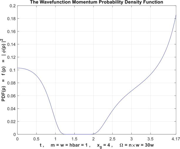
Figure 3.

The graph of the PDF as a function of the random variable T of the wavefunction momentum probability density for n = 30.

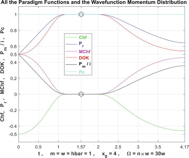
Figure 4.

The graphs of all the CPP parameters for the wavefunction momentum probability distribution as functions of the random variable T for n = 30.

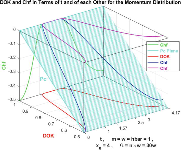
Figure 5.

The graphs of DOK and Chf and the deterministic probability Pc for the wavefunction momentum probability distribution in terms of T and of each other for n = 30.

Figure 6.

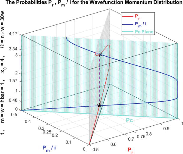
The graphs of P_r and P_m/i and Pc for the wavefunction momentum probability distribution in terms of T and of each other for n = 30.

Figure 7.

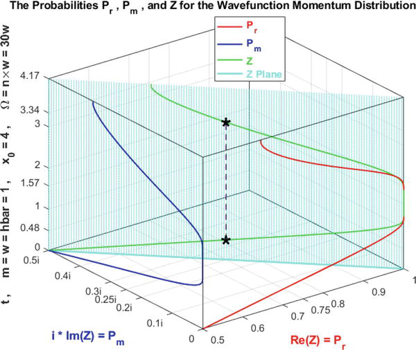
The graphs of the probabilities P_r and P_m and Z for the wavefunction momentum probability distribution in terms of T for n = 30.

Figure 8.

The graph of the PDF of the random variable T of the wavefunction momentum probability density as a function for n = 100.

Figure 9.

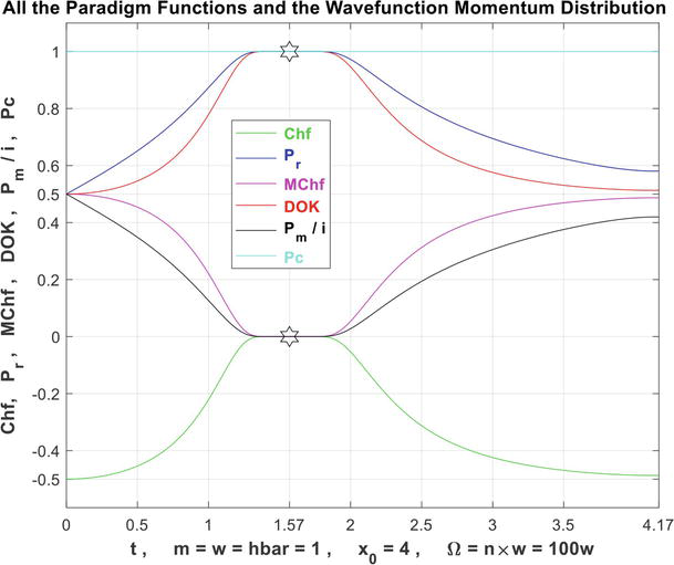
The graphs of all the CPP parameters for the wavefunction momentum probability distribution as functions of the random variable T for n = 100.

Figure 10.

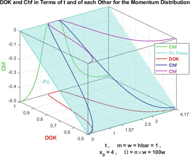
The graphs of DOK and Chf and the deterministic probability Pc for the wavefunction momentum probability distribution in terms of T and of each other for n = 100.

Figure 11.

The graphs of P_r and P_m/i and Pc for the wavefunction momentum probability distribution in terms of T and of each other for n = 100.

Figure 12.

The graphs of the probabilities P_r and P_m and Z for the wavefunction momentum probability distribution in terms of T for n = 100.

Figure 13.

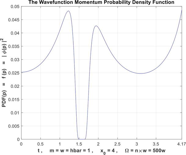
The graph of the PDF of the random variable T of the wavefunction momentum probability density as a function for n = 500.

Figure 14.

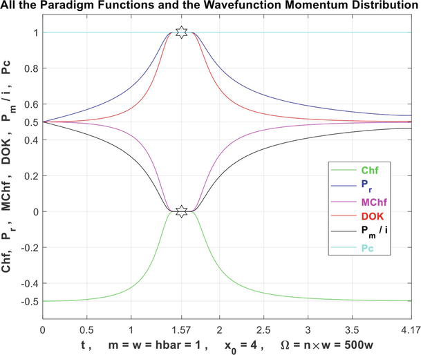
The graphs of all the CPP parameters for the wavefunction momentum probability distribution as functions of the random variable T for n = 500.

Figure 15.

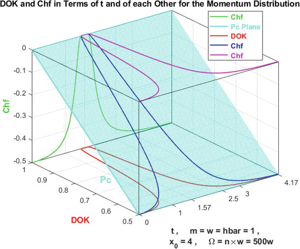
The graphs of DOK and Chf and the deterministic probability Pc for the wavefunction momentum probability distribution in terms of T and of each other for n = 500.

Figure 16.

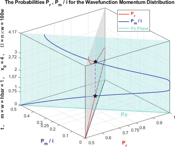
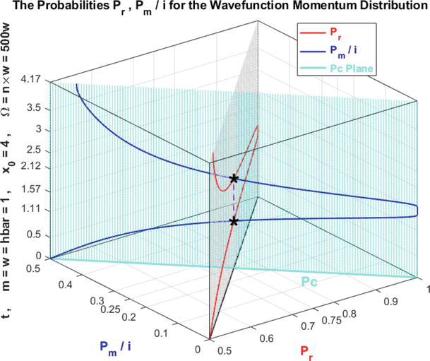
The graphs of P_r and P_m/i and Pc for the wavefunction momentum probability distribution in terms of T and of each other for n = 500.

Figure 17.

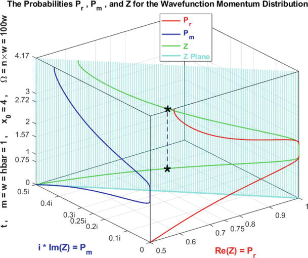
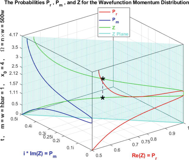
The graphs of the probabilities P_r and P_m and Z for the wavefunction momentum probability distribution in terms of T for n = 500.

4.2.1 Simulations interpretation

In Figures 3, 8, and 13, we can see the graphs of the probability density functions (PDF) of the wavefunction momentum probability distribution for this problem as functions of the time random variable $T:0\le T\le 4.17$ for n = 30, 100, 500.

In Figures 4, 9, and 14, we can see also the graphs and the simulations of all the CPP parameters (Chf, MChf, DOK, P_r, P_m/i, Pc) as functions of the time random variable T for the wavefunction momentum probability distribution of the quantum harmonic oscillators with Gaussian initial condition problem for n = 30, 100, 500. Hence, we can visualize all the new paradigm functions for this problem.

In the cubes (Figures 5, 10, and 15), the simulation of DOK and Chf as functions of each other and of the time random variable T for the quantum harmonic oscillators with Gaussian initial condition problem wavefunction momentum probability distribution can be seen. The thick line in cyan is the projection of the plane Pc²(T) = DOK(T) – Chf(T) = 1 = Pc(T) on the plane T = L_b = lower bound of T = 0. This thick line starts at the point (DOK = 0.5, Chf = −0.5) when T = L_b = 0, reaches the point (DOK = 1 Chf = 0) when T = 1.57, and returns at the end to (DOK = 0.5, Chf = −0.5) when T = U_b = upper bound of T = 4.17. The other curves are the graphs of DOK(T) (red) and Chf(T) (green, blue, pink) in different simulation planes. Notice that they all have a maximum at the point (DOK = 1, Chf = 0, T = 1.57). The last simulation point corresponds to (DOK = 0.5, Chf = −0.5, T = U_b = 4.17).

In the cubes (Figures 6, 11, and 16), we can notice the simulation of the real probability P_r(T) in $\mathcal{R}$ and its complementary real probability P_m(T)/i in $\mathcal{R}$ also in terms of the time random variable T for the quantum harmonic oscillators with Gaussian initial condition problem wavefunction momentum probability distribution. The thick line in cyan is the projection of the plane Pc²(T) = P_r(T) + P_m(T)/i = 1 = Pc(T) on the plane T = L_b = lower bound of T = 0. This thick line starts at the point (P_r = 0.5, P_m/i = 0.5) and ends at the point (P_r = 1, P_m/i = 0). The red curve represents P_r(T) in the plane P_r(T) = P_m(T)/i + 0.5 in light gray. This curve starts at the point (P_r = 0.5, P_m/i = 0, T = L_b = lower bound of T = 0), reaches the point (P_r = 1, P_m/i = 0.5, T = 1.57), and gets at the end to (P_r = 0.5, P_m/i = 0, T = U_b = upper bound of T = 4.17). The blue curve represents P_m(T)/i in the plane in cyan Pc²(T) = P_r(T) + P_m(T)/i = 1 = Pc(T). This curve starts at the point (P_r = 0.5, P_m/i = 0.5, T = L_b = lower bound of T = 0), reaches the point (P_r = 1, P_m/i = 0, T = 1.57), and gets at the end to (P_r = 0.5, P_m/i = 0.5, T = U_b = upper bound of T = 4.17). Notice the importance of the point which is on the intersection of the gray and cyan planes at T = 1.57 and when P_r(T) = 0.75 and P_m(T)/i = 0.25.

In the cubes (Figures 7, 12, and 17), we can notice the simulation of the complex probability Z(T) in $\mathcal{C}=\mathcal{R}+\mathcal{M}$ as a function of the real probability P_r(T) = Re(Z) in $\mathcal{R}$ and of its complementary imaginary probability P_m(T) = i × Im(Z) in $\mathcal{M}$, and this is in terms of the time random variable T for the quantum harmonic oscillators with Gaussian initial condition problem wavefunction momentum probability distribution. The red curve represents P_r(T) in the plane P_m(T) = 0 and the blue curve represents P_m(T) in the plane P_r(T) = 0.5. The green curve represents the complex probability Z(T) = P_r(T) + P_m(T) = Re(Z) + i × Im(Z) in the plane P_r(T) = iP_m(T) + 1 or Z(T) plane in cyan. The curve of Z(T) starts at the point (P_r = 0.5, P_m = 0.5i, T = L_b = lower bound of T = 0), reaches the point (P_r = 1, P_m/i = 0, T = 1.57), and ends at the point (P_r = 0.5, P_m = 0.5i, T = U_b = upper bound of T = 4.17). The thick line in cyan is P_r(T = L_b = 0) = iP_m(T = L_b = 0) + 1 and it is the projection of the Z(T) curve on the complex probability plane whose equation is: T = L_b = 0. This projected thick line starts at the point (P_r = 0.5, P_m = 0.5i, T = L_b = 0) and ends at the point (P_r = 1, P_m = 0, T = L_b = 0). Notice the importance of the point corresponding to T = 1.57 and Z = 0.75 + 0.25i when P_r = 0.75 and P_m = 0.25i.

Furthermore, as it was verified and proved and shown in this original paradigm (CPP) simulations, before the beginning of the simulation of the random event and at its end we have the chaotic factor (Chf and MChf) is 0 and the degree of our knowledge (DOK) is 1 since the stochastic and probabilistic effects and fluctuations have either not started yet or they have finished and terminated their task on the random phenomenon. During the execution of the nondeterministic experiment and process we also have: −0.5 ≤ Chf < 0, 0 < MChf ≤ 0.5, and 0.5 ≤ DOK < 1. We can see that during the whole and entire process we have constantly and incessantly ${\mathit{Pc}}^2=\mathit{DOK}-\mathit{Chf}=\mathit{DOK}+\mathit{\text{MChf}}=1=\mathit{Pc}$ that shows that the simulation which behaved probabilistically and randomly in the real universe and set $\mathcal{R}$ is now deterministic and certain in the complex probability universe and set $\mathcal{C}=\mathcal{R}+\mathcal{M}$ of CPP, and this after adding to the stochastic phenomenon performed in the real universe and set $\mathcal{R}$ the contributions of the imaginary universe and set $\mathcal{M}$ and thus after subtracting and eliminating from the degree of our knowledge the chaotic factor.

Finally, we can conclude that the quantum harmonic oscillator is the quantum-mechanical analog of the classical harmonic oscillator. Because an arbitrary smooth potential can usually be approximated as a harmonic potential at the vicinity of a stable equilibrium point, it is one of the most important model systems in quantum mechanics. Additionally, it is one of the few quantum-mechanical systems for which an exact and analytical solution is known [1, 2, 3]. Hence, we can see directly from all the simulations done and achieved that its relation to CPP is very fruitful, fascinating, and wonderful and which leads to delightful results and successful consequences.

4.3 The characteristics of the momentum probability distribution

In this quantum mechanics problem [20], the average, or expectation value of the momentum of a particle is given by:

$$⟨p⟩=\underset{0}{\overset{+\infty }{\int }}t{\left|\varphi \left(p,t\right)\right|}^2\mathit{dt}=\underset{0}{\overset{+\infty }{\int }}t\mathbb{N}\left(-{\mathit{mx}}_{0}wsin\left(\mathit{wt}\right),\sqrt{\frac{\mathrm{\hslash }m\mathrm{\Omega }}{2}\left({cos}^2\left(\mathit{wt}\right)+\frac{w^2}{{\mathrm{\Omega }}^2}{sin}^2\left(\mathit{wt}\right)\right)}\right)\mathit{dt}$$E21

For this problem, it can be shown that the average momentum is always $⟨p⟩=-{\mathit{mx}}_{0}wsin\left(\mathit{wt}\right)$.

So, in the probability set and universe $\mathcal{R}$, we have:

$${⟨p⟩}_R=⟨p⟩=-{\mathit{mx}}_{0}wsin\left(\mathit{wt}\right)$$E22

The variance in the momentum is a measure of the uncertainty in position of the particle, so in the probability set and universe $\mathcal{R}$, we have:

$${\mathrm{Var}}_{p,R}=\mathrm{Var}\left(p\right)={⟨p^2⟩}_R-{⟨p⟩}_R^2$$E23

$$=\left\{\underset{0}{\overset{+\infty }{\int }}{t}^2{\left|\varphi \left(p,t\right)\right|}^2\mathit{dt}\right\}-{\left\{\underset{0}{\overset{+\infty }{\int }}t{\left|\varphi \left(p,t\right)\right|}^2\mathit{dt}\right\}}^2$$E24

$$\begin{array}{l}=\left\{\underset{0}{\overset{+\infty }{\int }}{t}^2\mathbb{N}\left(-{\mathit{mx}}_{0}wsin\left(\mathit{wt}\right),\sqrt{\frac{\mathrm{\hslash }m\mathrm{\Omega }}{2}\left({cos}^2\left(\mathit{wt}\right)+\frac{w^2}{{\mathrm{\Omega }}^2}{sin}^2\left(\mathit{wt}\right)\right)}\right)\mathit{dt}\right\}-{\left[-{\mathit{mx}}_{0}wsin\left(\mathit{wt}\right)\right]}^2\\ =\frac{\mathrm{\hslash }m\mathrm{\Omega }}{2}\left({cos}^2\left(\mathit{wt}\right)+\frac{w^2}{{\mathrm{\Omega }}^2}{sin}^2\left(\mathit{wt}\right)\right)\end{array}$$E25

In the probability set and universe $\mathcal{M}$, we have:

$$\begin{array}{l}{⟨p⟩}_M=\underset{0}{\overset{+\infty }{\int }}t\left\{i\left[1-{\left|\varphi \left(p,t\right)\right|}^2\right]\right\}\mathit{dt}\\ =i\underset{0}{\overset{+\infty }{\int }}t\left\{1-\mathbb{N}\left(-{\mathit{mx}}_{0}wsin\left(\mathit{wt}\right),\sqrt{\frac{\mathrm{\hslash }m\mathrm{\Omega }}{2}\left({cos}^2\left(\mathit{wt}\right)+\frac{w^2}{{\mathrm{\Omega }}^2}{sin}^2\left(\mathit{wt}\right)\right)}\right)\right\}\mathit{dt}\\ =i\left\{\underset{0}{\overset{U_b}{\int }}\mathit{tdt}-\underset{0}{\overset{+\infty }{\int }}t\mathbb{N}\left(-{\mathit{mx}}_{0}wsin\left(\mathit{wt}\right),\sqrt{\frac{\mathrm{\hslash }m\mathrm{\Omega }}{2}\left({cos}^2\left(\mathit{wt}\right)+\frac{w^2}{{\mathrm{\Omega }}^2}{sin}^2\left(\mathit{wt}\right)\right)}\right)\mathit{dt}\right\}=i\left\{{\left[\frac{t^2}{2}\right]}_0^{U_b}-{⟨p⟩}_R\right\}\\ =i\left\{\frac{U_b^2}{2}-\left[-{\mathit{mx}}_{0}wsin\left(\mathit{wt}\right)\right]\right\}=i\left\{\frac{U_b^2}{2}+{\mathit{mx}}_{0}wsin\left(\mathit{wt}\right)\right\}\end{array}$$E26

Where $U_b$ is the upper bound of the definite integral above. Practically, the standard normal distribution probability is very nearly equal to 1.0000 (0.99997 exactly) for $U_b=4$.

Note that, $\text{If}{U}_b\to +\infty \iff {⟨p⟩}_M\to +\infty$. Moreover,

$$\begin{array}{l}{\mathrm{Var}}_{p,M}={⟨p^2⟩}_M-{⟨p⟩}_M^2=\left\{\underset{0}{\overset{+\infty }{\int }}{t}^2\left\{i\left[1-{\left|\varphi \left(p,t\right)\right|}^2\right]\right\}\mathit{dt}\right\}-{\left\{\underset{0}{\overset{+\infty }{\int }}t\left\{i\left[1-{\left|\varphi \left(p,t\right)\right|}^2\right]\right\}\mathit{dt}\right\}}^2\\ =i\underset{0}{\overset{+\infty }{\int }}{t}^2\left\{1-\mathbb{N}\left(-{\mathit{mx}}_{0}wsin\left(\mathit{wt}\right),\sqrt{\frac{\mathrm{\hslash }m\mathrm{\Omega }}{2}\left({cos}^2\left(\mathit{wt}\right)+\frac{w^2}{{\mathrm{\Omega }}^2}{sin}^2\left(\mathit{wt}\right)\right)}\right)\right\}\mathit{dt}-{\left\{i\left[\frac{U_b^2}{2}+{\mathit{mx}}_{0}wsin\left(\mathit{wt}\right)\right]\right\}}^2\end{array}$$E27

$$\begin{array}{l}=i\left\{\underset{0}{\overset{U_b}{\int }}{t}^2\mathit{dt}-\underset{0}{\overset{+\infty }{\int }}{t}^2\left\{\mathbb{N}\left(-{\mathit{mx}}_{0}wsin\left(\mathit{wt}\right),\sqrt{\frac{\mathrm{\hslash }m\mathrm{\Omega }}{2}\left({cos}^2\left(\mathit{wt}\right)+\frac{w^2}{{\mathrm{\Omega }}^2}{sin}^2\left(\mathit{wt}\right)\right)}\right)\right\}\mathit{dt}\right\}\\ +{\left\{\frac{U_b^2}{2}+{\mathit{mx}}_{0}wsin\left(\mathit{wt}\right)\right\}}^2\end{array}$$E28

$$=i\left\{\underset{0}{\overset{U_b}{\int }}{t}^2\mathit{dt}-{\mathrm{Var}}_{p,R}\right\}+{\left\{\frac{U_b^2}{2}+{\mathit{mx}}_{0}wsin\left(\mathit{wt}\right)\right\}}^2=i\left\{{\left[\frac{t^3}{3}\right]}_0^{U_b}-{\mathrm{Var}}_{p,R}\right\}+{\left\{\frac{U_b^2}{2}+{\mathit{mx}}_{0}wsin\left(\mathit{wt}\right)\right\}}^2$$E29

$$=i\left\{\frac{U_b^3}{3}-\frac{\mathrm{\hslash }m\mathrm{\Omega }}{2}\left({cos}^2\left(\mathit{wt}\right)+\frac{w^2}{{\mathrm{\Omega }}^2}{sin}^2\left(\mathit{wt}\right)\right)\right\}+{\left\{\frac{U_b^2}{2}+{\mathit{mx}}_{0}wsin\left(\mathit{wt}\right)\right\}}^2$$E30

Note that, $\text{If}{U}_b\to +\infty \iff {\mathrm{Var}}_{p,M}\to +\infty$.

In the probability set and the universe $\mathcal{C}=\mathcal{R}+\mathcal{M}$, we have from CPP:

$$\begin{array}{l}{⟨p⟩}_C=\underset{0}{\overset{+\infty }{\int }}t\left[z\left(p,t\right)\right]\mathit{dt}=\underset{0}{\overset{+\infty }{\int }}t\left\{{\left|\varphi \left(p,t\right)\right|}^2+i\left[1-{\left|\varphi \left(p,t\right)\right|}^2\right]\right\}\mathit{dt}\\ =\underset{0}{\overset{+\infty }{\int }}t{\left|\varphi \left(p,t\right)\right|}^2\mathit{dt}+\underset{0}{\overset{+\infty }{\int }}t\left\{i\left[1-{\left|\varphi \left(p,t\right)\right|}^2\right]\right\}\mathit{dt}\\ =\underset{0}{\overset{+\infty }{\int }}t\mathbb{N}\left(-{\mathit{mx}}_{0}wsin\left(\mathit{wt}\right),\sqrt{\frac{\mathrm{\hslash }m\mathrm{\Omega }}{2}\left({cos}^2\left(\mathit{wt}\right)+\frac{w^2}{{\mathrm{\Omega }}^2}{sin}^2\left(\mathit{wt}\right)\right)}\right)\mathit{dt}\\ +i\underset{0}{\overset{+\infty }{\int }}t\left\{1-\mathbb{N}\left(-{\mathit{mx}}_{0}wsin\left(\mathit{wt}\right),\sqrt{\frac{\mathrm{\hslash }m\mathrm{\Omega }}{2}\left({cos}^2\left(\mathit{wt}\right)+\frac{w^2}{{\mathrm{\Omega }}^2}{sin}^2\left(\mathit{wt}\right)\right)}\right)\right\}\mathit{dt}\\ ={⟨p⟩}_R+{⟨p⟩}_M=-{\mathit{mx}}_{0}wsin\left(\mathit{wt}\right)+i\left\{\frac{U_b^2}{2}+{\mathit{mx}}_{0}wsin\left(\mathit{wt}\right)\right\}\end{array}$$E31

Note that, $\text{If}{U}_b\to +\infty \iff {⟨p⟩}_C\to +\infty$.

$$\begin{array}{l}{\mathrm{Var}}_{p,C}={⟨p^2⟩}_C-{⟨p⟩}_C^2=\left[\underset{0}{\overset{+\infty }{\int }}{t}^2\left[z\left(p,t\right)\right]\mathit{dt}\right]-{\left[{⟨p⟩}_R+{⟨p⟩}_M\right]}^2\\ =\left[\underset{0}{\overset{+\infty }{\int }}{t}^2\left\{{\left|\varphi \left(p,t\right)\right|}^2+i\left[1-{\left|\varphi \left(p,t\right)\right|}^2\right]\right\}\mathit{dt}\right]-{\left[{⟨p⟩}_R+{⟨p⟩}_M\right]}^2\\ =\left[\underset{0}{\overset{+\infty }{\int }}{t}^2{\left|\varphi \left(p,t\right)\right|}^2\mathit{dt}+\underset{0}{\overset{+\infty }{\int }}{t}^2\left\{i\left[1-{\left|\varphi \left(p,t\right)\right|}^2\right]\right\}\mathit{dt}\right]-{\left[{⟨p⟩}_R+{⟨p⟩}_M\right]}^2\\ =\left[{⟨p^2⟩}_R+{⟨p^2⟩}_M\right]-{\left[{⟨p⟩}_R+{⟨p⟩}_M\right]}^2=\left[{⟨p^2⟩}_R+{⟨p^2⟩}_M\right]-\left[{⟨p⟩}_R^2+{⟨p⟩}_M^2+2{⟨p⟩}_R{⟨p⟩}_M\right]\\ =\left[{⟨p^2⟩}_R-{⟨p⟩}_R^2\right]+\left[{⟨p^2⟩}_M-{⟨p⟩}_M^2\right]-2{⟨p⟩}_R{⟨p⟩}_M={\mathrm{Var}}_{p,R}+{\mathrm{Var}}_{p,M}-2{⟨p⟩}_R{⟨p⟩}_M\\ =\frac{\mathrm{\hslash }m\mathrm{\Omega }}{2}\left({cos}^2\left(\mathit{wt}\right)+\frac{w^2}{{\mathrm{\Omega }}^2}{sin}^2\left(\mathit{wt}\right)\right)+i\left\{\frac{U_b^3}{3}-\frac{\mathrm{\hslash }m\mathrm{\Omega }}{2}\left({cos}^2\left(\mathit{wt}\right)+\frac{w^2}{{\mathrm{\Omega }}^2}{sin}^2\left(\mathit{wt}\right)\right)\right\}\\ +{\left\{\frac{U_b^2}{2}+{\mathit{mx}}_{0}wsin\left(\mathit{wt}\right)\right\}}^2-2\left\{-{\mathit{mx}}_{0}wsin\left(\mathit{wt}\right)\right\}\times \left\{i\left\{\frac{U_b^2}{2}+{\mathit{mx}}_{0}wsin\left(\mathit{wt}\right)\right\}\right\}\end{array}$$E32

Note that, $\text{If}{U}_b\to +\infty \iff {\mathrm{Var}}_{p,C}\to +\infty$.

The following tables (Tables 1–4) compute the momentum distribution characteristics for $x_0=4$, $m=w=\mathrm{\hslash }=1$, $n=1/4$ where $\mathrm{\Omega }=n\times w$, and $U_b=6,20,50,1000$.

Momentum distribution characteristics	$x_0=4$, $m=w=\mathrm{\hslash }=1$, $\mathrm{\Omega }=w/4$, $U_b=6$
${⟨p⟩}_R$	1.1177
${\mathrm{Var}}_{p,R}$	0.2714
${⟨p⟩}_M$	i × 16.8823
${\mathrm{Var}}_{p,M}$	285.0133 + i × 71.7286
${⟨p⟩}_C={⟨p⟩}_R+{⟨p⟩}_M$	1.1177 + i × 16.8823
${\mathrm{Var}}_{p,C}={\mathrm{Var}}_{p,R}+{\mathrm{Var}}_{p,M}-2{⟨p⟩}_R{⟨p⟩}_M$	285.2847 + i × 33.9911

Table 1.

The momentum distribution characteristics for $U_b=6$ and $n=1/4$.

Momentum distribution characteristics	$x_0=4$, $m=w=\mathrm{\hslash }=1$, $\mathrm{\Omega }=w/4$, $U_b=20$
${⟨p⟩}_R$	$-3.6518$
${\mathrm{Var}}_{p,R}$	1.6878
${⟨p⟩}_M$	i × 203.6518
${\mathrm{Var}}_{p,M}$	4.1474e+04 + i × 2.6650e+03
${⟨p⟩}_C={⟨p⟩}_R+{⟨p⟩}_M$	$-3.6518$ + i × 203.6518
${\mathrm{Var}}_{p,C}={\mathrm{Var}}_{p,R}+{\mathrm{Var}}_{p,M}-2{⟨p⟩}_R{⟨p⟩}_M$	4.1476e+04 + i × 4.1524e+03

Table 2.

The momentum distribution characteristics for $U_b=20$ and $n=1/4$_.

Momentum distribution characteristics	$x_0=4$, $m=w=\mathrm{\hslash }=1$, $\mathrm{\Omega }=w/4$, $U_b=50$
${⟨p⟩}_R$	1.0495
${\mathrm{Var}}_{p,R}$	0.2541
${⟨p⟩}_M$	i × 1.2490e+03
${\mathrm{Var}}_{p,M}$	1.5599e+06 + i × 4.1666e+04
${⟨p⟩}_C={⟨p⟩}_R+{⟨p⟩}_M$	1.0495 + i × 1.2490e+03
${\mathrm{Var}}_{p,C}={\mathrm{Var}}_{p,R}+{\mathrm{Var}}_{p,M}-2{⟨p⟩}_R{⟨p⟩}_M$	1.5599e+06 + i × 3.9045 + 04

Table 3.

The momentum distribution characteristics for $U_b=50$ and $n=1/4$_.

Momentum distribution characteristics	$x_0=4$, $m=w=\mathrm{\hslash }=1$, $\mathrm{\Omega }=w/4$, $U_b=1000$
${⟨p⟩}_R$	$-3.3075$
${\mathrm{Var}}_{p,R}$	1.4070
${⟨p⟩}_M$	i × 5.0000e+05
${\mathrm{Var}}_{p,M}$	2.5000e+11 + i × 3.3333e+08
${⟨p⟩}_C={⟨p⟩}_R+{⟨p⟩}_M$	$-3.3075$ + i × 5.0000e+05
${\mathrm{Var}}_{p,C}={\mathrm{Var}}_{p,R}+{\mathrm{Var}}_{p,M}-2{⟨p⟩}_R{⟨p⟩}_M$	2.5000e+11 + i × 3.3664 + 08

Table 4.

The momentum distribution characteristics for $U_b=1000$ and $n=1/4$_.

5. The quantum uncertainty principle in $\mathcal{R}$, $\mathcal{M}$, and$\mathcal{C}$

Copying the variances above and applying trigonometric identities [1, 2, 3], we can write the product of the standard deviations as:

$$\begin{array}{l}{\sigma }_{x_R}\times {\sigma }_{p_R}=\sqrt{{\mathrm{Var}}_{x,R}}\times \sqrt{{\mathrm{Var}}_{p,R}}\\ =\sqrt{\frac{\mathrm{\hslash }}{2m\mathrm{\Omega }}\left({cos}^2\left(\mathit{wt}\right)+\frac{{\mathrm{\Omega }}^2}{w^2}{sin}^2\left(\mathit{wt}\right)\right)}\times \sqrt{\frac{\mathrm{\hslash }m\mathrm{\Omega }}{2}\left({cos}^2\left(\mathit{wt}\right)+\frac{w^2}{{\mathrm{\Omega }}^2}{sin}^2\left(\mathit{wt}\right)\right)}\\ =\frac{\mathrm{\hslash }}{2}\sqrt{\left({cos}^2\left(\mathit{wt}\right)+\frac{{\mathrm{\Omega }}^2}{w^2}{sin}^2\left(\mathit{wt}\right)\right)\left({cos}^2\left(\mathit{wt}\right)+\frac{w^2}{{\mathrm{\Omega }}^2}{sin}^2\left(\mathit{wt}\right)\right)}\\ =\frac{\mathrm{\hslash }}{4}\sqrt{3+\frac{1}{2}\left(\frac{{\mathrm{\Omega }}^2}{w^2}+\frac{w^2}{{\mathrm{\Omega }}^2}\right)-\left(\frac{1}{2}\left(\frac{{\mathrm{\Omega }}^2}{w^2}+\frac{w^2}{{\mathrm{\Omega }}^2}\right)-1\right)cos\left(4\mathit{wt}\right)}\end{array}$$E33

Since $\forall \left(w,t\right)\in {ℝ}^2:{cos}^2\left(\mathit{wt}\right)+{sin}^2\left(\mathit{wt}\right)=1$.

and $cos\left(4\mathit{wt}\right)=2{cos}^2\left(2\mathit{wt}\right)-1=1-2{sin}^2\left(2\mathit{wt}\right)$.

and $sin\left(2\mathit{wt}\right)=2sin\left(\mathit{wt}\right)cos\left(\mathit{wt}\right)$.

which are the half angles formulas.

From the relations:

$\frac{{\mathrm{\Omega }}^2}{w^2}+\frac{w^2}{{\mathrm{\Omega }}^2}\ge 2$ and $\forall \left(w,t\right)\in {ℝ}^2:-1\le cos\left(4\mathit{wt}\right)\le 1\iff 0\le \left|cos\left(4\mathit{wt}\right)\right|\le 1$.

Then:

$${\sigma }_{x_R}\times {\sigma }_{p_R}\ge \frac{\mathrm{\hslash }}{4}\sqrt{3+\frac{1}{2}\left(\frac{{\mathrm{\Omega }}^2}{w^2}+\frac{w^2}{{\mathrm{\Omega }}^2}\right)-\left(\frac{1}{2}\left(\frac{{\mathrm{\Omega }}^2}{w^2}+\frac{w^2}{{\mathrm{\Omega }}^2}\right)-1\right)}=\frac{\mathrm{\hslash }}{2}$$E34

which obeys the quantum uncertainty principle in the probability set and universe $\mathcal{R}$.

The uncertainties in the probability set and universe $\mathcal{M}$ in position and momentum (${\sigma }_{x_M}$ and ${\sigma }_{p_M}$) are defined as being equal to the square root of their respective variances in $\mathcal{M}$, so that:

$${\sigma }_{x_M}\times {\sigma }_{p_M}=\sqrt{{\mathrm{Var}}_{x,M}}\times \sqrt{{\mathrm{Var}}_{p,M}}\to \sqrt{+\infty }\times \sqrt{+\infty }\to +\infty$$E35

$\iff {\sigma }_{x_M}\times {\sigma }_{p_M}\ge \frac{\mathrm{\hslash }}{2}$, in accordance with the quantum uncertainty principle.

The uncertainties in the probability set and universe $\mathcal{C}$ = $\mathcal{R}+\mathcal{M}$ in position and momentum (${\sigma }_{x_C}$ and ${\sigma }_{p_C}$) are defined as being equal to the square root of their respective variances in $\mathcal{C}$, so that:

$${\sigma }_{x_C}\times {\sigma }_{p_C}=\sqrt{{\mathrm{Var}}_{x,C}}\times \sqrt{{\mathrm{Var}}_{p,C}}\to \sqrt{+\infty }\times \sqrt{+\infty }\to +\infty$$E36

$\iff {\sigma }_{x_C}\times {\sigma }_{p_C}\ge \frac{\mathrm{\hslash }}{2}$, in accordance with the quantum uncertainty principle.

Consequently, the quantum uncertainty principle is verified in the universe $\mathcal{R}$, in the universe $\mathcal{M}$, and in the complex universe $\mathcal{C}=\mathcal{R}+\mathcal{M}$.

6. The wavefunction entropies in $\mathcal{R},\mathcal{M},$and $\mathcal{C}$

Another measure of uncertainty in position is the Shannon information entropy of the probability distribution $H_x$ which is the entropy in $\mathcal{R}$ and is equal to [1, 2, 3, 4, 5, 6, 7, 8, 9, 10, 11, 12, 13, 14, 15, 16, 17, 18, 19, 20, 21, 22, 23, 24, 25, 26, 27, 28, 29, 30, 31, 32, 33, 34, 35, 36]:

$$H_x=-\underset{0}{\overset{+\infty }{\int }}{\left|\psi \left(x,t\right)\right|}^2\mathit{Ln}\left[{\left|\psi \left(x,t\right)\right|}^{2}x{\text{'}}_0\right]\mathit{dt}=-\underset{0}{\overset{U_b}{\int }}{\left|\psi \left(x,t\right)\right|}^2\mathit{Ln}\left[{\left|\psi \left(x,t\right)\right|}^{2}x{\text{'}}_0\right]\mathit{dt}$$E37

Where $U_b$ is the upper bound of the definite integral above. Practically, the standard normal distribution probability is very nearly equal to 1.0000 (0.99997 exactly) for $U_b=4$.

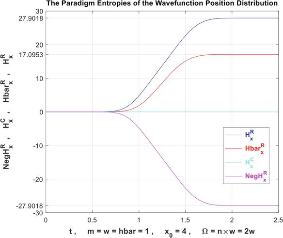
$=-\sum _{t=0}^{t=U_b}{\left|\psi \left(x,t\right)\right|}^2\mathit{Ln}\left[{\left|\psi \left(x,t\right)\right|}^{2}x{\text{'}}_0\right]=H_x^R$ with $\mathit{dt}=0.01$ and where $x{\text{'}}_0$ is an arbitrary reference length.

Take $x{\text{'}}_0=1\iff H_x^R=-\sum _{t=0}^{t=U_b}{\left|\psi \left(x,t\right)\right|}^2\mathit{Ln}\left[{\left|\psi \left(x,t\right)\right|}^2\right]$.

$\iff \forall t:0\le t<+\infty ,\text{we have}:d\left[H_x^R\right]\ge 0$, that means that $H_x^R$ is a nondecreasing series with time t and converging and that also in $\mathcal{R}$, chaos and disorder are increasing with time t.

The negative real entropy corresponding to $H_x^R$ in $\mathcal{R}$ is ${\mathit{\text{NegH}}}_x^R$ and is the following:

$${\mathit{\text{NegH}}}_x^R=-H_x^R=\sum _{t=0}^{t=U_b}{\left|\psi \left(x,t\right)\right|}^2\mathit{Ln}\left[{\left|\psi \left(x,t\right)\right|}^2\right]$$E38

$\iff \forall t:0\le t<+\infty ,\text{we have}:d\left[{\mathit{\text{NegH}}}_x^R\right]\le 0$, that means that ${\mathit{\text{NegH}}}_x^R$ is a nonincreasing series with time t and converging. Therefore, if $H_x^R$ measures in $\mathcal{R}$ the amount of disorder, of uncertainty, of chaos, of ignorance, of unpredictability, and of information gain in a random system then since ${\mathit{\text{NegH}}}_x^R=-H_x^R$, that means the opposite of $H_x^R$, ${\mathit{\text{NegH}}}_x^R$ measures in $\mathcal{R}$ the amount of order, of certainty, of predictability, and of information loss in a stochastic system.

The complementary real entropy to $H_x^R$ in $\mathcal{R}$ is ${\overline{H}}_x^R$ and is the following:

$${\overline{H}}_x^R=-\sum _{t=0}^{t=U_b}\left[1-{\left|\psi \left(x,t\right)\right|}^2\right]\mathit{Ln}\left[1-{\left|\psi \left(x,t\right)\right|}^2\right]$$E39

In the complementary real probability set to $\mathcal{R}$, we denote the corresponding real entropy by ${\overline{H}}_x^R$.

The meaning of ${\overline{H}}_x^R$ is the following: It is the real entropy in the real set $\mathcal{R}$ and which is related to the complementary real probability $P_m/i=1-P_r$.

$\iff \forall t:0\le t<+\infty ,\text{we have}:d\left[{\overline{H}}_x^R\right]\ge 0$, that means that ${\overline{H}}_x^R$ is a nondecreasing series with time t and converging and that also means that in the complementary real probability set to $\mathcal{R}$, chaos and disorder are increasing with time t.

In the complementary imaginary probability set $\mathcal{M}$ to the set $\mathcal{R}$, we denote the corresponding imaginary entropy by $H_x^M$. The meaning of $H_x^M$ is the following: It is the imaginary entropy in the imaginary set $\mathcal{M}$ and which is related to the complementary imaginary probability $P_m=i\left(1-P_r\right)$. The complementary entropy to $H_x^R$ in $\mathcal{M}$ is $H_x^M$ and is computed as follows:

$$\begin{array}{l}{H}_x^M=-\sum _{t=0}^{t=U_b}i\left[1-{\left|\psi \left(x,t\right)\right|}^2\right]\mathit{Ln}\left\{i\left[1-{\left|\psi \left(x,t\right)\right|}^2\right]\right\}\\ =-\sum _{t=0}^{t=U_b}i\left[1-{\left|\psi \left(x,t\right)\right|}^2\right]\left\{\mathit{Lni}+\mathit{Ln}\left[1-{\left|\psi \left(x,t\right)\right|}^2\right]\right\}\\ =-\sum _{t=0}^{t=U_b}i\left\{\mathit{Lni}+\mathit{Ln}\left[1-{\left|\psi \left(x,t\right)\right|}^2\right]-\left[{\left|\psi \left(x,t\right)\right|}^2\right]\mathit{Lni}-\left[{\left|\psi \left(x,t\right)\right|}^2\right]\mathit{Ln}\left[1-{\left|\psi \left(x,t\right)\right|}^2\right]\right\}\\ =-\sum _{t=0}^{t=U_b}\mathit{\text{iLni}}+\mathit{iLn}\left[1-{\left|\psi \left(x,t\right)\right|}^2\right]-i\left[{\left|\psi \left(x,t\right)\right|}^2\right]\mathit{Lni}-i\left[{\left|\psi \left(x,t\right)\right|}^2\right]\mathit{Ln}\left[1-{\left|\psi \left(x,t\right)\right|}^2\right]\\ =-\sum _{t=0}^{t=U_b}\mathit{\text{iLni}}\left[1-{\left|\psi \left(x,t\right)\right|}^2\right]+i\left[1-{\left|\psi \left(x,t\right)\right|}^2\right]\mathit{Ln}\left[1-{\left|\psi \left(x,t\right)\right|}^2\right]\\ =-\sum _{t=0}^{t=U_b}\mathit{\text{iLni}}\left[1-{\left|\psi \left(x,t\right)\right|}^2\right]-i\sum _{t=0}^{t=U_b}\left[1-{\left|\psi \left(x,t\right)\right|}^2\right]\mathit{Ln}\left[1-{\left|\psi \left(x,t\right)\right|}^2\right]\\ =-\sum _{t=0}^{t=U_b}\mathit{\text{iLni}}\left[1-{\left|\psi \left(x,t\right)\right|}^2\right]+i{\overline{H}}_x^R=-\mathit{\text{iLni}}\sum _{t=0}^{t=U_b}\left[1-{\left|\psi \left(x,t\right)\right|}^2\right]+i{\overline{H}}_x^R\\ =-\mathit{\text{iLni}}\left\{\sum _{t=0}^{t=U_b}1-\sum _{t=0}^{t=U_b}{\left|\psi \left(x,t\right)\right|}^2\right\}+i{\overline{H}}_x^R\\ =-\mathit{\text{iLni}}\left\{\left[\left(U_b-0\right)+1\right]-1\right\}+i{\overline{H}}_x^R\text{since}\sum _{t=0}^{t=U_b}{\left|\psi \left(x,t\right)\right|}^2=1\\ =-\left(\mathit{\text{iLni}}\right)U_b+i{\overline{H}}_x^R\end{array}$$E40

From the properties of logarithms, we have: $\mathit{\text{θLnx}}=\mathit{Ln}\left(x^{\theta }\right)$ then $\mathit{\text{iLni}}={\mathit{Lni}}^i$.

Moreover, Leonhard Euler’s formula for complex numbers gives:

$$e^{\mathit{i\theta }}=cos\theta +isin\theta$$E41

Take $\theta =\pi /2+2\mathit{k\pi }\iff e^{i\left(\pi /2+2\mathit{k\pi }\right)}=cos\left(\pi /2+2\mathit{k\pi }\right)+isin\left(\pi /2+2\mathit{k\pi }\right)=0+i\left(1\right)=i$, then:

$i^i={\left(e^{i\left(\pi /2+2\mathit{k\pi }\right)}\right)}^i=e^{i^2\left(\pi /2+2\mathit{k\pi }\right)}=e^{-\left(\pi /2+2\mathit{k\pi }\right)}$ since i²=−1, therefore:

$-\mathit{\text{iLni}}=-{\mathit{Lni}}^i=-\mathit{Ln}\left[e^{-\left(\pi /2+2\mathit{k\pi }\right)}\right]=\pi /2+2\mathit{k\pi }$ since $\mathit{Ln}\left[e\right]=1$ and where $k$ belongs to the set of integer numbers $\mathbb{Z}$.

Consequently,

$$H_x^M=-\left(\mathit{\text{iLni}}\right)U_b+i{\overline{H}}_x^R=\left(\pi /2+2\mathit{k\pi }\right)U_b+i{\overline{H}}_x^R$$E42

That means that $H_x^M$ is a complex number where:

the real part is: $Re\left(H_x^M\right)=\left(\pi /2+2\mathit{k\pi }\right)U_b$.

and the imaginary part is: $Im\left(H_x^M\right)={\overline{H}}_x^R$.

For $k=-1$ then $Re\left(H_x^M\right)=\left(-3\pi /2\right)U_b=-4.71238898U_b=-18.84955592\dots \text{for}{U}_b=4$.

For $k=0$ then $Re\left(H_x^M\right)=\left(\pi /2\right)U_b=1.570796327U_b=6.283185307\dots \text{for}{U}_b=4$.

For $k=1$ then $Re\left(H_x^M\right)=\left(5\pi /2\right)U_b=7.853981634U_b=31.41592654\dots \text{for}{U}_b=4$.

etc.…

Finally, the entropy $H_x^C$ in $\mathcal{C}$ = $\mathcal{R}+\mathcal{M}$ is the following:

$$\begin{array}{l}{H}_x^C=-\sum _{t=0}^{t=U_b}\mathit{Pc}\left(t\right)\mathit{Ln}\left[\mathit{Pc}\left(t\right)\right]\\ =-\sum _{t=0}^{t=U_b}1\times \mathit{Ln}\left[1\right]=-\sum _{t=0}^{t=U_b}\left(1\times 0\right)=0\\ =H_x^R+{\mathit{\text{NegH}}}_x^R\end{array}$$E43

$\iff \forall t:0\le t<+\infty ,\text{we have}:d\left[H_x^C\right]=0$, that means that $H_x^C$ is a constant series with time t and is always equal to 0. That means also and most importantly, for the wavefunction position distribution and in the probability set and universe $\mathcal{C}=\mathcal{R}+\mathcal{M}$, we have complete order, no chaos, no ignorance, no uncertainty, no disorder, no randomness, no information loss or gain but a conservation of information, and no unpredictability since all measurements are completely and perfectly deterministic ($\mathit{Pc}\left(t\right)=1$ and $H_x^C=0$).

Similarly, we can determine another measure of uncertainty in momentum which is the information entropy of the probability distribution $H_p$ and which is:

$$H_p=-\underset{0}{\overset{+\infty }{\int }}{\left|\varphi \left(p,t\right)\right|}^2\mathit{Ln}\left[{\left|\varphi \left(p,t\right)\right|}^{2}p{\text{'}}_0\right]\mathit{dt}=-\underset{0}{\overset{U_b}{\int }}{\left|\varphi \left(p,t\right)\right|}^2\mathit{Ln}\left[{\left|\varphi \left(p,t\right)\right|}^{2}p{\text{'}}_0\right]\mathit{dt}$$E44

where $U_b$ is the upper bound of the definite integral above. Practically, the standard normal distribution probability is very nearly equal to 1.0000 (0.99997 exactly) for $U_b=4$.

$=-\sum _{t=0}^{t=U_b}{\left|\varphi \left(p,t\right)\right|}^2\mathit{Ln}\left[{\left|\varphi \left(p,t\right)\right|}^{2}p{\text{'}}_0\right]$ with $\mathit{dt}=0.01$ and where $p{\text{'}}_0$ is an arbitrary reference momentum.

For $p{\text{'}}_0=1$ we can compute similarly all the defined entropies in $\mathcal{R}$, $\mathcal{M}$, and $\mathcal{C}$ and which are:

$$H_p^R=-\sum _{t=0}^{t=U_b}{\left|\varphi \left(p,t\right)\right|}^2\mathit{Ln}\left[{\left|\varphi \left(p,t\right)\right|}^2\right]$$E45

$${\mathit{\text{NegH}}}_p^R=\sum _{t=0}^{t=U_b}{\left|\varphi \left(p,t\right)\right|}^2\mathit{Ln}\left[{\left|\varphi \left(p,t\right)\right|}^2\right]$$E46

$${\overline{H}}_p^R=-\sum _{t=0}^{t=U_b}\left[1-{\left|\varphi \left(p,t\right)\right|}^2\right]\mathit{Ln}\left[1-{\left|\varphi \left(p,t\right)\right|}^2\right]$$E47

$$H_p^M=-\sum _{t=0}^{t=U_b}i\left[1-{\left|\varphi \left(p,t\right)\right|}^2\right]\mathit{Ln}\left\{i\left[1-{\left|\varphi \left(p,t\right)\right|}^2\right]\right\}=\left(\pi /2+2\mathit{k\pi }\right)U_b+i{\overline{H}}_p^R$$E48

$$\begin{array}{l}{H}_p^C=-\sum _{t=0}^{t=U_b}\mathit{Pc}\left(t\right)\mathit{Ln}\left[\mathit{Pc}\left(t\right)\right]=-\sum _{t=0}^{t=U_b}1\times \mathit{Ln}\left[1\right]=-\sum _{t=0}^{t=U_b}\left(1\times 0\right)=0\\ =H_p^R+{\mathit{\text{NegH}}}_p^R\end{array}$$E49

That means also and most importantly, for the wavefunction momentum distribution and in the probability set and universe $\mathcal{C}=\mathcal{R}+\mathcal{M}$, we have complete order, no chaos, no ignorance, no uncertainty, no disorder, no randomness, no information loss or gain but a conservation of information, and no unpredictability since all measurements are completely and perfectly deterministic ($\mathit{Pc}\left(t\right)=1$ and $H_p^C=0$).

Due to the Fourier transform relation between the position wavefunction $\psi \left(x\right)$ and the momentum wavefunction $\varphi \left(p\right)$, the above constraint can be written for the corresponding entropies as:

$H_x+H_p\ge \mathit{Ln}\left(\frac{\mathit{eh}}{2x{\text{'}}_{0}p{\text{'}}_0}\right)$, where h is Planck’s constant.

Depending on one’s choice of the $x{\text{'}}_{0}p{\text{'}}_0$ product, the expression may be written in many ways. If $x{\text{'}}_{0}p{\text{'}}_0$ is chosen to be h, then:

$$H_x+H_p\ge \mathit{Ln}\left(\frac{e}{2}\right)$$E50

If, instead, $x{\text{'}}_{0}p{\text{'}}_0$ is chosen to be $\mathrm{\hslash }$, then:

$$H_x+H_p\ge \mathit{Ln}\left(\mathit{e\pi }\right)$$E51

If $x{\text{'}}_0$ and $p{\text{'}}_0$ are chosen to be unity in whatever system of units are being used, then:

$$H_x+H_p\ge \mathit{Ln}\left(\frac{\mathit{eh}}{2}\right)$$E52

where h is interpreted as a dimensionless number equal to the value of Planck’s constant in the chosen system of units.

The following figures (Figures 18–29) illustrate all the computations done above.

Figure 18.

The graphs of $H_x^R,{\overline{H}}_x^R,H_x^C,{\mathit{\text{NegH}}}_x^R$ as functions of T for $n=2$.

Figure 19.

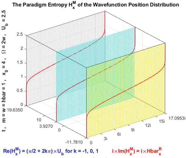
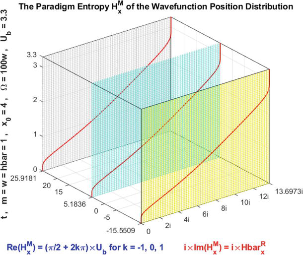
The graph of $H_x^M=Re\left(H_x^M\right)+iIm\left(H_x^M\right)$ in red as functions of T for $n=2$ and for $k=-1,0,1$ in the planes in yellow, in cyan, and in light gray, respectively.

Figure 20.

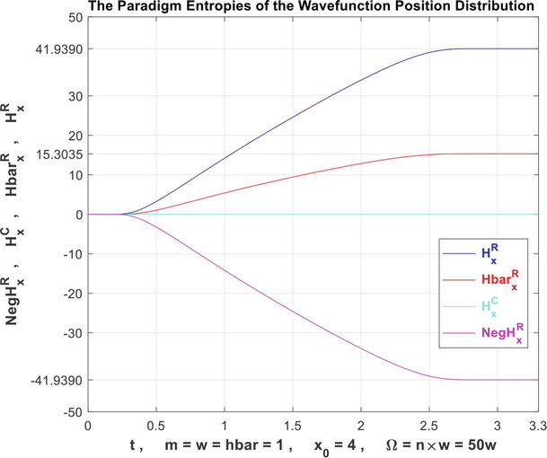
The graphs of $H_x^R,{\overline{H}}_x^R,H_x^C,{\mathit{\text{NegH}}}_x^R$ as functions of T for $n=50$.

Figure 21.

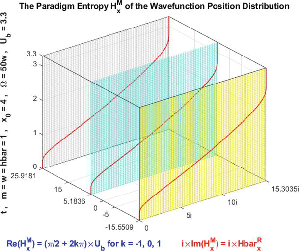
The graph of $H_x^M=Re\left(H_x^M\right)+iIm\left(H_x^M\right)$ in red as functions of T for $n=50$ and for $k=-1,0,1$ in the planes in yellow, in cyan, and in light gray, respectively.

Figure 22.

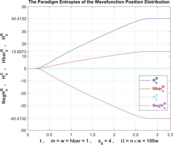
The graphs of $H_x^R,{\overline{H}}_x^R,H_x^C,{\mathit{\text{NegH}}}_x^R$ as functions of T for $n=100$.

Figure 23.

The graph of $H_x^M=Re\left(H_x^M\right)+iIm\left(H_x^M\right)$ in red as functions of T for $n=100$ and for $k=-1,0,1$ in the planes in yellow, in cyan, and in light gray, respectively.

Figure 24.

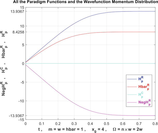
The graphs of $H_p^R,{\overline{H}}_p^R,H_p^C,{\mathit{\text{NegH}}}_p^R$ as functions of T for $n=2$.

Figure 25.

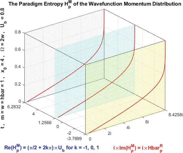
The graph of $H_p^M=Re\left(H_p^M\right)+iIm\left(H_p^M\right)$ in red as functions of T for $n=2$ and for $k=-1,0,1$ in the planes in yellow, in cyan, and in light gray, respectively.

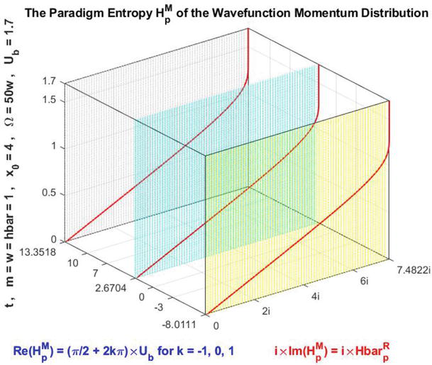
Figure 26.

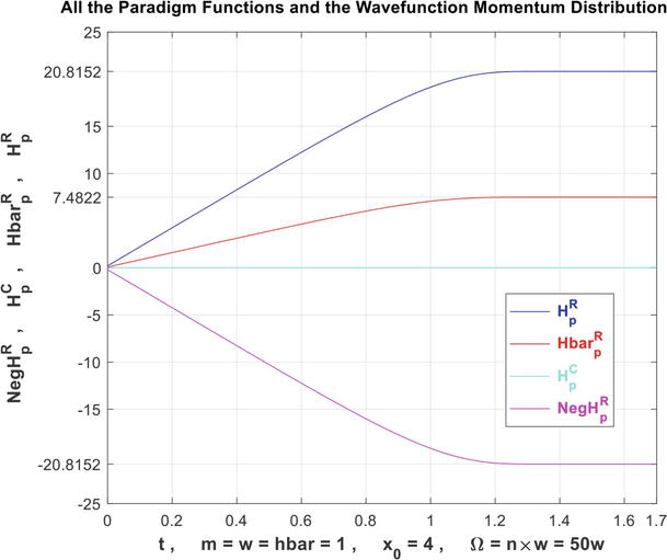
The graphs of $H_p^R,{\overline{H}}_p^R,H_p^C,{\mathit{\text{NegH}}}_p^R$ as functions of T for $n=50$.

Figure 27.

The graph of $H_p^M=Re\left(H_p^M\right)+iIm\left(H_p^M\right)$ in red as functions of T for $n=50$ and for $k=-1,0,1$ in the planes in yellow, in cyan, and in light gray, respectively.

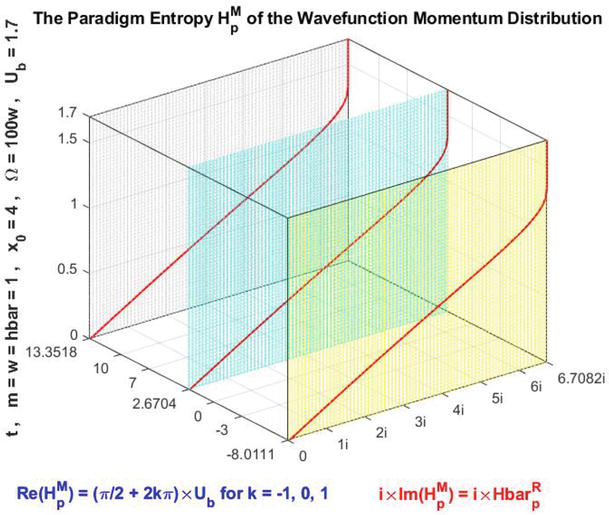
Figure 28.

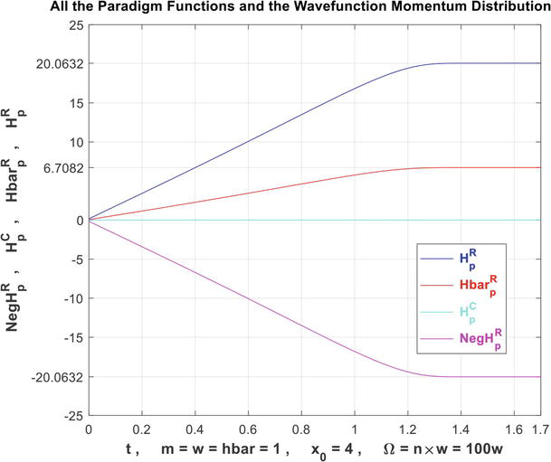
The graphs of $H_p^R,{\overline{H}}_p^R,H_p^C,{\mathit{\text{NegH}}}_p^R$ as functions of T for $n=100$.

Figure 29.

The graph of $H_p^M=Re\left(H_p^M\right)+iIm\left(H_p^M\right)$ in red as functions of T for $n=100$ and for $k=-1,0,1$ in the planes in yellow, in cyan, and in light gray, respectively.

7. Conclusion and perspectives

In the current research work, the original extended model of eight axioms (EKA) of A. N. Kolmogorov was connected and applied to the quantum harmonic oscillators with Gaussian initial condition problem in quantum mechanics theory. Thus, a tight link between quantum mechanics and the novel paradigm (CPP) was achieved. Consequently, the model of “Complex Probability” was more developed beyond the scope of my 23 previous research works on this topic. We can realize that during this whole process we have continually and incessantly ${\mathit{Pc}}^2=\mathit{DOK}-\mathit{Chf}=\mathit{DOK}+\mathit{\text{MChf}}=1=\mathit{Pc}$, that means that the simulation which behaved stochastically and randomly in the real universe and probability set $\mathcal{R}$ is now deterministic and certain in the complex probability universe and set $\mathcal{C}=\mathcal{R}+\mathcal{M}$. This is accomplished by adding to the stochastic phenomenon occurring in the real probability universe $\mathcal{R}$ the contributions of the imaginary probability universe and set $\mathcal{M}$ and hence after subtracting and eliminating from the degree of our knowledge the chaotic factor. Additionally, the real, imaginary, complex, and deterministic probabilities that correspond to each value of the momentum random variable have been evaluated in the three probabilities universes and sets which are $\mathcal{R}$, $\mathcal{M}$, and $\mathcal{C}$ by $P_r$, $P_m$, Z and Pc, respectively. Consequently, at each value of time t, the novel quantum mechanics and CPP parameters P_r, P_m, $P_m/i$, DOK, Chf, MChf, Pc, and Z are perfectly and surely evaluated and predicted in the complex probabilities universe and set $\mathcal{C}$ with Pc maintained equal to 1 repeatedly and permanently. Furthermore, we are successful to visualize and to quantify both the system certain knowledge (expressed and materialized by DOK and Pc) and the chaos and stochastic influences and effects (expressed and materialized by Chf and MChf) of the new paradigm when referring to all these obtained graphs and executed simulations throughout the whole research work. This is certainly very wonderful, fascinating, and fruitful and shows and proves once again the rewards of extending the five axioms of probability of A. N. Kolmogorov and thus the benefits and novelty of my original and novel model in the fields of applied mathematics, prognostics, and quantum mechanics that can be called verily: “The Complex Probability Paradigm.” As a prospective and future research and challenges, we aim to more elaborate the novel prognostic paradigm developed and to apply it to a wide set of nondeterministic and stochastic phenomena in quantum mechanics theory.

Conflicts of interest

The author declares that there are no conflict of interests regarding the publication of this work.

Data availability

The data used to support the findings of this study are available from the author upon request.

Nomenclature

$\mathcal{R}$

probabilities and events real set

$\mathcal{M}$

probabilities and events imaginary set

$\mathcal{C}$

probabilities and events complex set

i

the imaginary number where $i^2=-1$ or $i=\sqrt{-1}$

EKA

Extended Kolmogorov’s Axioms

CPP

Complex Probability Paradigm

P_rob

any event probability

P_r

probability of an event in the real set $\mathcal{R}$

P_m

probability of an event in the imaginary set $\mathcal{M}$ associated with the real probability in $\mathcal{R}$

Pc

probability of an event in $\mathcal{R}$ with its corresponding complementary event in $\mathcal{M}$ = probability in the complex probability set $\mathcal{C}=\mathcal{R}+\mathcal{M}$

Z

complex probability number = sum of P_r and P_m = complex random vector

DOK

$={\left|Z\right|}^2$= the random experiment or system degree of our knowledge, it is the square of the norm of Z

Chf

the chaotic factor of Z

MChf

the magnitude of the chaotic factor of Z

${\left|\psi \left(x,t\right)\right|}^2$

probability density function of the position wavefunction

${\left|\varphi \left(p,t\right)\right|}^2$

probability density function of the momentum wavefunction

${⟨x⟩}_R$,${⟨x⟩}_M$,${⟨x⟩}_C$

averages, or expectations, or means of the position wavefunction probability density function in $\mathcal{R}$, $\mathcal{M}$, and $\mathcal{C},$ respectively

${\mathrm{Var}}_{x,R}$,${\mathrm{Var}}_{x,M}$,${\mathrm{Var}}_{x,C}$

variances of the position wavefunction probability density function in $\mathcal{R}$, $\mathcal{M}$, and $\mathcal{C},$respectively

${⟨p⟩}_R$,${⟨p⟩}_M$,${⟨p⟩}_C$

averages, or expectations, or means of the momentum wavefunction probability density function in $\mathcal{R}$, $\mathcal{M}$, and $\mathcal{C},$ respectively

${\mathrm{Var}}_{p,R}$,${\mathrm{Var}}_{p,M}$,${\mathrm{Var}}_{p,C}$

variances of the momentum wavefunction probability density function in $\mathcal{R}$, $\mathcal{M}$, and $\mathcal{C},$ respectively

$H_x^R$

entropy in the real universe $\mathcal{R}$ of the particle position

${\mathit{\text{NegH}}}_x^R$

negative entropy in the real universe $\mathcal{R}$ of the particle position

${\overline{H}}_x^R$

complementary entropy in the real universe $\mathcal{R}$ of the particle position

$H_x^M$

entropy in the imaginary universe $\mathcal{M}$ of the particle position

$H_x^C$

entropy in the complex universe $\mathcal{C}$ of the particle position

$H_p^R$

entropy in the real universe $\mathcal{R}$ of the particle momentum

${\mathit{\text{NegH}}}_p^R$

negative entropy in the real universe $\mathcal{R}$ of the particle momentum

${\overline{H}}_p^R$

complementary entropy in the real universe $\mathcal{R}$ of the particle momentum

$H_p^M$

entropy in the imaginary universe $\mathcal{M}$ of the particle momentum

$H_p^C$

entropy in the complex universe $\mathcal{C}$ of the particle momentum