The Paradigm of Complex Probability and Quantum Mechanics: The Quantum Harmonic Oscillator with Gaussian Initial Condition – The Position Wavefunction

Abstract

In the current work, we extend and incorporate the five-axioms probability system of Andrey Nikolaevich Kolmogorov, set up in 1933 the imaginary set of numbers, and this by adding three supplementary axioms. Consequently, any stochastic experiment can thus be achieved in the extended complex probabilities set $\mathcal{C}$ which is the sum of the real probabilities set $\mathcal{R}$ and the imaginary probabilities set $\mathcal{M}$. The purpose here is to evaluate the complex probabilities by considering additional novel imaginary dimensions to the experiment occurring in the “real” laboratory. Therefore, the random phenomenon outcome and result in $\mathcal{C}=\mathcal{R}+\mathcal{M}$ can be predicted absolutely and perfectly no matter what the random distribution of the input variable in $\mathcal{R}$ is since the associated probability in the entire set $\mathcal{C}$ is constantly and permanently equal to one. Thus, the following consequence indicates that chance and randomness in $\mathcal{R}$ are replaced now by absolute and total determinism in $\mathcal{C}$ as a result of subtracting from the degree of our knowledge of the chaotic factor in the probabilistic experiment. Moreover, I will apply to the established theory of quantum mechanics my original complex probability paradigm (CPP) in order to express the quantum mechanics problem considered here completely deterministically in the universe of probabilities $\mathcal{C}=\mathcal{R}+\mathcal{M}$.

1. Introduction

The theory of quantum mechanics provides a description of nature physical properties at the scale of atoms and subatomic particles and is a fundamental theory in physics. Quantum mechanics is the foundation of all quantum physics, including quantum field theory, quantum chemistry, quantum information science, and quantum technology [1, 2, 3, 4, 5, 6, 7, 8, 9, 10, 11, 12, 13].

Classical physics differs from quantum mechanics since in the latter, we have that angular momentum, momentum, energy, and other quantities of a bound system are limited to discrete values (quantization), and there are restrictions to how accurately the physical quantity value can be determined and predicted prior to its measurement given a complete set of initial conditions (the uncertainty principle), and objects have characteristics of waves and particles (wave–particle duality).

The theory of quantum mechanics was developed progressively from theories to explain observations that could not be explained by classical physics, such as the black-body radiation problem solution proposed by Max Planck’s in 1900 and the explanation of the photoelectric by Albert Einstein’s 1905 paper as a correspondence between energy and frequency. The full development of quantum mechanics in the mid-1920s by Niels Bohr, Max Born, Werner Heisenberg, Erwin Schrödinger, and others were the early attempts to explain and understand microscopic phenomena and which is now known as the “old quantum theory.” Various specially developed mathematical formalisms formulate the modern theory of quantum mechanics. In one of these invented formalisms, a mathematical entity named the wave function provides in the form of probability amplitudes the information about what measurements of a particle’s momentum, energy, and other physical properties may give.

Moreover, the quantum-mechanical analog of the classical harmonic oscillator is the quantum harmonic oscillator. It is one of the most important model systems in quantum mechanics because an arbitrary smooth potential can generally be estimated as a harmonic potential at the neighborhood of a stable equilibrium point. Furthermore, since an exact, analytical solution is known, it is one of the few quantum-mechanical systems for which this kind of solution is provided.

Consequently, I will relate my complex probability paradigm (CPP) to this well-known and important problem in quantum mechanics in order to express it completely deterministically.

In the end, and to conclude, this research work is organized as follows: in Section 1, we will present the introduction, then in Section 2, we will explain the advantages and the purpose of the present work. Afterward, in Section 3, we will explain and summarize the extended Kolmogorov’s axioms and hence present the original parameters and interpretation of the complex probability paradigm. Additionally, in Section 4, the quantum harmonic oscillators with the Gaussian initial condition problem will be related to the new paradigm after applying CPP in the first chapter to the position wavefunction and then in the following second chapter to the momentum wavefunction of the problem. Hence, some corresponding simulations will be achieved, and subsequently, the characteristics of these random distributions will be evaluated in the probabilities sets $\mathcal{R}$, $\mathcal{M}$, and $\mathcal{C}$. Finally, in Section 5, a comprehensive summary concludes the work. Then, we will present the list of references mentioned and cited in the current research work.

2. The purpose and the advantages of the current publication

Computing probabilities is all our work in the classical theory of probability. Adding new dimensions to our stochastic experiment is an innovative idea in the current paradigm, making the study absolutely deterministic. As a matter of fact, the theory of probability is a nondeterministic theory by essence which means that all the random events outcome is due to luck and chance. Hence, we make the study deterministic by adding new imaginary dimensions to the phenomenon occurring in the “real” laboratory, which is $\mathcal{R}$, and therefore a stochastic experiment will have a certain outcome in the complex probabilities set $\mathcal{C}$. It is of great significance that random systems become completely predictable since we will be perfectly knowledgeable to predict the outcome of all stochastic and chaotic phenomena that occur in nature, for example, in all stochastic processes, in statistical mechanics, or in the well-established field of quantum mechanics. Consequently, the work that should be done is to add the contributions of $\mathcal{M},$ which is the set of imaginary probabilities, to the set of real probabilities$\mathcal{R}$ that will make the random phenomenon in $\mathcal{C}=\mathcal{R}+\mathcal{M}$ completely deterministic. Since this paradigm is found to be fruitful, then a new theory in prognostic and stochastic sciences is established, and this is to understand deterministically those events that used to be stochastic events in $\mathcal{R}$. This is what I coined by the term “The Complex Probability Paradigm” that was elaborated and initiated in my 23 previous papers [14, 15, 16, 17, 18, 19, 20, 21, 22, 23, 24, 25, 26, 27, 28, 29, 30, 31, 32, 33, 34, 35, 36].

To summarize, the advantages and the purposes of this current work and chapter are to:

1. Relate probability theory to the field of complex variables and analysis in mathematics and, therefore, to extend the theory of classical probability to the set of complex numbers. This task was elaborated and initiated in my 23 previous papers.

2. Apply the novel probability axioms and CPP paradigm to quantum mechanics, specifically to the quantum harmonic oscillators with Gaussian initial condition problem.

3. Demonstrate that any stochastic and random event and experiment can be expressed deterministically in the complex probabilities set$\mathcal{C}$.

4. Quantify both the chaos magnitude and the degree of our knowledge of the wavefunction position distribution and CPP in the sets $\mathcal{R}$, $\mathcal{M}$, and $\mathcal{C}$.

5. Represent graphically and illustrate the parameters and functions of the original paradigm related to this quantum mechanics problem.

6. Evaluate all the characteristics of the wavefunction position distribution.

7. Demonstrate that the classical concepts of the stochastic system have a probability of occurring permanently equal to one in the complex set; consequently, no ignorance, no unpredictability, no stochasticity, no disorder, no randomness, no nondeterminism, and no chaos exist in:

   $$\mathcal{C}\left(\text{complex}\mathrm{set}\right)=\mathcal{R}\left(\text{real}\mathrm{set}\right)+\mathcal{M}\left(\text{imaginary}\mathrm{set}\right)$$E1

8. Prepare to apply the novel paradigm to other topics in stochastic processes, in statistical mechanics, and to the field of prognostics in science, engineering, and quantum mechanics. This will be the task in my following research work and publications.

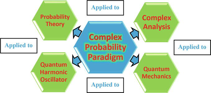
Compared with existing literature, the major contribution of the current research work is to apply the novel paradigm of CPP to quantum mechanics and to express it completely deterministically. And concerning some applications of the novel developed paradigm, and as a future work, it can be applied to any nondeterministic phenomenon in quantum mechanics. The next figure displays the major purposes of the complex probability paradigm (CPP) (Figure 1).

Figure 1.

The diagram of the Complex Probability Paradigm applied to Quantum Mechanics major purposes and goals.

3. The complex probability paradigm

3.1 The original Andrey Nikolaevich Kolmogorov system of axioms

The simplicity of Kolmogorov’s system of axioms may be surprising [14, 15, 16, 17, 18, 19, 20, 21, 22, 23, 24, 25, 26, 27, 28, 29, 30, 31, 32, 33, 34, 35, 36]. Let E be a collection of elements {E₁, E₂, …} called elementary events, and let F be a set of subsets of E called random events [37, 38, 39, 40, 41]. The five axioms for a finite set E are:

1. Axiom 1: F is a field of sets.

2. Axiom 2: F contains the set E.

3. Axiom 3: A nonnegative real number P_rob(A), called the probability of A, is assigned to each set A in F. We always have 0 ≤ P_rob(A) ≤ 1.

4. Axiom 4: P_rob(E) equals 1.

5. Axiom 5: If A and B have no elements in common, the number assigned to their union is:

$$P_{\mathit{rob}}\left(A\cup B\right)=P_{\mathit{rob}}\left(A\right)+P_{\mathit{rob}}\left(B\right)$$E2

hence, we say that A and B are disjoint; otherwise, we have:

$$P_{\mathit{rob}}\left(A\cup B\right)=P_{\mathit{rob}}\left(A\right)+P_{\mathit{rob}}\left(B\right)-P_{\mathit{rob}}\left(A\cap B\right)$$E3

And we also say that: $P_{\mathit{rob}}\left(A\cap B\right)=P_{\mathit{rob}}\left(A\right)\times P_{\mathit{rob}}\left(B/A\right)=P_{\mathit{rob}}\left(B\right)\times P_{\mathit{rob}}\left(A/B\right)$ which is the conditional probability. If both A and B are independent, then: $P_{\mathit{rob}}\left(A\cap B\right)=P_{\mathit{rob}}\left(A\right)\times P_{\mathit{rob}}\left(B\right)$.

Moreover, we can generalize and say that for N disjoint (mutually exclusive) events $A_1,A_2,\dots ,A_j,\dots ,A_N$ (for $1\le j\le N$), we have the following additivity rule:

$$P_{\mathit{rob}}\left(\bigcup _{j=1}^N{A}_j\right)=\sum _{j=1}^N{P}_{\mathit{rob}}\left(A_j\right)$$E4

And we also say that for N independent events $A_1,A_2,\dots ,A_j,\dots ,A_N$ (for $1\le j\le N$), we have the following product rule:

$$P_{\mathit{rob}}\left(\bigcap _{j=1}^N{A}_j\right)=\prod _{j=1}^N{P}_{\mathit{rob}}\left(A_j\right)$$E5

3.2 Adding the imaginary part $\mathcal{M}$

Now, we can add to this system of axioms an imaginary part such that:

1. Axiom 6: Let $P_m=i\times \left(1-P_r\right)$ be the probability of an associated complementary event in $\mathcal{M}$ (the imaginary part or universe) to the event A in $\mathcal{R}$ (the real part or universe). It follows that $P_r+P_m/i=1$ where i is the imaginary number with $i=\sqrt{-1}$ or $i^2=-1$.

2. Axiom 7: We construct the complex number or vector $Z=P_r+P_m=P_r+i\left(1-P_r\right)$ having a norm $\left|Z\right|$ such that:

$${\left|Z\right|}^2=P_r^2+{\left(P_m/i\right)}^2.$$E6

1. Axiom 8: Let Pc denote the probability of an event in the complex probability set and universe $\mathcal{C}$ where $\mathcal{C}=\mathcal{R}+\mathcal{M}$. We say that Pc is the probability of an event A in $\mathcal{R}$ with its associated and complementary event in $\mathcal{M}$ such that:

$${\mathit{Pc}}^2={\left(P_r+P_m/i\right)}^2={\left|Z\right|}^2-2{\mathit{iP}}_r{P}_m\text{and is always equal to}1.$$E7

We can see that by taking into consideration the set of imaginary probabilities we added three new and original axioms and consequently the system of axioms defined by Kolmogorov was hence expanded to encompass the set of imaginary numbers and realm [42, 43, 44, 45, 46, 47, 48, 49, 50, 51, 52, 53, 54, 55, 56, 57, 58, 59, 60, 61, 62, 63, 64, 65].

3.3 A concise interpretation of the original CPP paradigm

To conclude and to summarize, we state that the degree of our certain knowledge is undesirably incomplete and imperfect and thus unsatisfactory in the real probability universe $\mathcal{R}$. Hence, we extend our study to the set of complex numbers $\mathcal{C},$ which includes the contributions of both the set of real probabilities which is $\mathcal{R}$ and the set of complementary imaginary probabilities which is $\mathcal{M}$. Consequently, this will result to a perfect and absolute degree of our knowledge in the probability universe $\mathcal{C}$= $\mathcal{R}$+ $\mathcal{M}$ because Pc = 1 continuously. In fact, the study in the complex universe $\mathcal{C}$ leads to a certain prediction of any stochastic and random event and experiment since in $\mathcal{C},$ we subtract and eliminate the measured chaotic factor from the computed degree of our knowledge. This will result in a probability permanently equal to 1 in the universe $\mathcal{C}$ as it is shown in the following equation deduced from CPP: ${\mathit{Pc}}^2=\mathit{DOK}-\mathit{Chf}=\mathit{DOK}+\mathit{\text{MChf}}=1=\mathit{Pc}$. Many numerous discrete and continuous probability distributions were illustrated in my 23 previous research works, and that confirm this hypothesis and original paradigm [14, 15, 16, 17, 18, 19, 20, 21, 22, 23, 24, 25, 26, 27, 28, 29, 30, 31, 32, 33, 34, 35, 36]. The Extended Kolmogorov Axioms (EKA for short) or the Complex Probability Paradigm (CPP for short) can be summarized and shown in the next illustration (Figure 2):

Figure 2.

The EKA or the CPP diagram.

4. The Quantum Harmonic Oscillator with Gaussian Initial Condition and the Complex Probability Paradigm (CPP) Parameters – The Position Wavefunction and CPP

In this section, we will relate and link quantum mechanics to the complex probability paradigm with all its parameters by applying it to the quantum harmonic oscillators with Gaussian initial condition and this by using the four CPP concepts, which are: the real probability $P_r$ in the real probability set $\mathcal{R}$, the imaginary probability $P_m$ in the imaginary probability set $\mathcal{M}$, the complex random vector or number $Z$ in the complex probability set $\mathcal{C}=\mathcal{R}+\mathcal{M}$, and the deterministic real probability $\mathit{Pc}$ also in the probability set $\mathcal{C}$ [1, 2, 3, 4, 5, 6, 7, 8, 9, 10, 11, 12, 13, 14, 15, 16, 17, 18, 19, 20, 21, 22, 23, 24, 25, 26, 27, 28, 29, 30, 31, 32, 33, 34, 35, 36, 66, 67, 68, 69, 70, 71, 72, 73, 74, 75, 76, 77, 78, 79, 80, 81, 82, 83, 84, 85, 86, 87, 88, 89, 90, 91, 92].

4.1 The position wavefunction solution

One significant quantum–theoretic periodic wave packet which has a ubiquitous presence in the arena of quantum optics and quantum electronics is the coherent state of the simple harmonic oscillator. This state evolves from the initial condition [1, 2, 3],

$$\mathrm{\Psi }\left(x,t=0\right)={\left(\frac{m\mathrm{\Omega }}{\pi \mathrm{\hslash }}\right)}^{1/4}exp\left(-\frac{m\mathrm{\Omega }{\left(x-x_0\right)}^2}{2\mathrm{\hslash }}\right)$$E8

where $w$ is the angular frequency and Ω is the width of the initial state, and where Ω is not necessarily equal to $w$. This equation has the form of simple Gaussian modeling of the ground (stationary) state of the harmonic oscillator but with an added feature: its center has $x_0$ the amount of displacement. Note that a coherent state is a Gaussian wave packet that does not flatten out over time since all the terms are in phase. Coherent states also sport another interesting feature: they satisfy the minimum uncertainty relation!

Integrating over the propagator eventually delivers [1, 2, 3]:

$${\left|\psi \left(x,t\right)\right|}^2\sim \mathbb{N}\left(x_{0}cos\left(\mathit{wt}\right),\sqrt{\frac{\mathrm{\hslash }}{2m\mathrm{\Omega }}\left({cos}^2\left(\mathit{wt}\right)+\frac{{\mathrm{\Omega }}^2}{w^2}{sin}^2\left(\mathit{wt}\right)\right)}\right)$$E9

where the notation $\mathbb{N}\left({\mu }_x,{\sigma }_x\right)$ is deployed, designating a normal distribution of mean ${\mu }_x=x_{0}cos\left(\mathit{wt}\right)$ with standard deviation ${\sigma }_x=\sqrt{\frac{\mathrm{\hslash }}{2m\mathrm{\Omega }}\left({cos}^2\left(\mathit{wt}\right)+\frac{{\mathrm{\Omega }}^2}{w^2}{sin}^2\left(\mathit{wt}\right)\right)}$. Knowing that we have taken in this study $\mathrm{\Omega }=n\times w$_, where $n$ is a simple multiplier and can be equal to ¼, or ½, or 1, or 2, or 50, or 100, or 300, etc., as it will be shown afterward in the simulations section.

4.2 The position wavefunction probability distribution and CPP

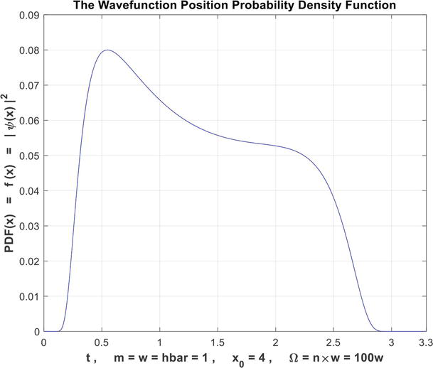
For the quantum harmonic oscillators with Gaussian initial condition, the wavefunction position probability density function (PDF) is given by:

$$f\left(x\right)={\left|\psi \left(x,t\right)\right|}^2=\mathbb{N}\left(x_{0}cos\left(\mathit{wt}\right),\sqrt{\frac{\mathrm{\hslash }}{2m\mathrm{\Omega }}\left({cos}^2\left(\mathit{wt}\right)+\frac{{\mathrm{\Omega }}^2}{w^2}{sin}^2\left(\mathit{wt}\right)\right)}\right)$$E10

Therefore, the wavefunction position cumulative probability distribution function (CDF), which is equal to $P_r\left(T\right)$ in $\mathcal{R}$ is:

$$\begin{array}{rcl}{P}_r\left(T\right)& =& F\left(t_j\right)=P_{\mathit{rob}}\left(T\le t_j\right)=\underset{0}{\overset{t_j}{\int }}{\left|\psi \left(x,t\right)\right|}^2\mathit{dt}\\ & =& \underset{0}{\overset{t_j}{\int }}\mathbb{N}\left(x_{0}cos\left(\mathit{wt}\right),\sqrt{\frac{\mathrm{\hslash }}{2m\mathrm{\Omega }}\left({cos}^2\left(\mathit{wt}\right)+\frac{{\mathrm{\Omega }}^2}{w^2}{sin}^2\left(\mathit{wt}\right)\right)}\right)\mathit{dt}\end{array}$$E11

And the real complementary probability to $P_r\left(T\right)$ in $\mathcal{R}$ which is $P_m\left(T\right)/i$ is:

$$P_m\left(T\right)/i=\begin{array}{l}1-P_r\left(T\right)=1-F\left(t_j\right)=1-P_{\mathit{rob}}\left(T\le t_j\right)=P_{\mathit{rob}}\left(T>t_j\right)=1-\underset{0}{\overset{t_j}{\int }}{\left|\psi \left(x,t\right)\right|}^2\mathit{dt}\\ =\underset{t_j}{\overset{+\infty }{\int }}{\left|\psi \left(x,t\right)\right|}^2\mathit{dt}\end{array}$$

$$\begin{array}{l}=1-\underset{0}{\overset{t_j}{\int }}\mathbb{N}\left(x_{0}cos\left(\mathit{wt}\right),\sqrt{\frac{\mathrm{\hslash }}{2m\mathrm{\Omega }}\left({cos}^2\left(\mathit{wt}\right)+\frac{{\mathrm{\Omega }}^2}{w^2}{sin}^2\left(\mathit{wt}\right)\right)}\right)\mathit{dt}\\ =\underset{t_j}{\overset{+\infty }{\int }}\mathbb{N}\left(x_{0}cos\left(\mathit{wt}\right),\sqrt{\frac{\mathrm{\hslash }}{2m\mathrm{\Omega }}\left({cos}^2\left(\mathit{wt}\right)+\frac{{\mathrm{\Omega }}^2}{w^2}{sin}^2\left(\mathit{wt}\right)\right)}\right)\mathit{dt}\end{array}$$E12

Consequently, the imaginary complementary probability to $P_r\left(T\right)$ in $\mathcal{M}$ which is $P_m\left(T\right)$ is:

$$\begin{array}{l}{P}_m\left(T\right)=i\left[1-P_r\left(T\right)\right]=i\left[1-F\left(t_j\right)\right]=i\left[1-P_{\mathit{rob}}\left(T\le t_j\right)\right]={\mathit{iP}}_{\mathit{rob}}\left(T>t_j\right)\\ =i\left[1-\underset{0}{\overset{t_j}{\int }}{\left|\psi \left(x,t\right)\right|}^2\mathit{dt}\right]=i\underset{t_j}{\overset{+\infty }{\int }}{\left|\psi \left(x,t\right)\right|}^2\mathit{dt}\\ =i\left[1-\underset{0}{\overset{t_j}{\int }}\mathbb{N}\left(x_{0}cos\left(\mathit{wt}\right),\sqrt{\frac{\mathrm{\hslash }}{2m\mathrm{\Omega }}\left({cos}^2\left(\mathit{wt}\right)+\frac{{\mathrm{\Omega }}^2}{w^2}{sin}^2\left(\mathit{wt}\right)\right)}\right)\mathit{dt}\right]\\ =i\underset{t_j}{\overset{+\infty }{\int }}\mathbb{N}\left(x_{0}cos\left(\mathit{wt}\right),\sqrt{\frac{\mathrm{\hslash }}{2m\mathrm{\Omega }}\left({cos}^2\left(\mathit{wt}\right)+\frac{{\mathrm{\Omega }}^2}{w^2}{sin}^2\left(\mathit{wt}\right)\right)}\right)\mathit{dt}\end{array}$$E13

Furthermore, the complex random number or vector in $\mathcal{C}=\mathcal{R}+\mathcal{M}$ which is $Z\left(T\right)$ is:

$$\begin{array}{l}Z\left(T\right)=P_r\left(T\right)+P_m\left(T\right)=P_r\left(T\right)+i\left[1-P_r\left(T\right)\right]=F\left(t_j\right)+i\left[1-F\left(t_j\right)\right]\\ =P_{\mathit{rob}}\left(T\le t_j\right)+i\left[1-P_{\mathit{rob}}\left(T\le t_j\right)\right]=P_{\mathit{rob}}\left(T\le t_j\right)+{\mathit{iP}}_{\mathit{rob}}\left(T>t_j\right)\\ =\left[\underset{0}{\overset{t_j}{\int }}{\left|\psi \left(x,t\right)\right|}^2\mathit{dt}\right]+i\left[1-\underset{0}{\overset{t_j}{\int }}{\left|\psi \left(x,t\right)\right|}^2\mathit{dt}\right]=\underset{0}{\overset{t_j}{\int }}{\left|\psi \left(x,t\right)\right|}^2\mathit{dt}+i\underset{t_j}{\overset{+\infty }{\int }}{\left|\psi \left(x,t\right)\right|}^2\mathit{dt}\end{array}$$

$$\begin{array}{l}=\left[\underset{0}{\overset{t_j}{\int }}\mathbb{N}\left(x_{0}cos\left(\mathit{wt}\right),\sqrt{\frac{\mathrm{\hslash }}{2m\mathrm{\Omega }}\left({cos}^2\left(\mathit{wt}\right)+\frac{{\mathrm{\Omega }}^2}{w^2}{sin}^2\left(\mathit{wt}\right)\right)}\right)\mathit{dt}\right]\\ +i\left[1-\underset{0}{\overset{t_j}{\int }}\mathbb{N}\left(x_{0}cos\left(\mathit{wt}\right),\sqrt{\frac{\mathrm{\hslash }}{2m\mathrm{\Omega }}\left({cos}^2\left(\mathit{wt}\right)+\frac{{\mathrm{\Omega }}^2}{w^2}{sin}^2\left(\mathit{wt}\right)\right)}\right)\mathit{dt}\right]\\ =\left[\underset{0}{\overset{t_j}{\int }}\mathbb{N}\left(x_{0}cos\left(\mathit{wt}\right),\sqrt{\frac{\mathrm{\hslash }}{2m\mathrm{\Omega }}\left({cos}^2\left(\mathit{wt}\right)+\frac{{\mathrm{\Omega }}^2}{w^2}{sin}^2\left(\mathit{wt}\right)\right)}\right)\mathit{dt}\right]\\ +i\left[\underset{t_j}{\overset{+\infty }{\int }}\mathbb{N}\left(x_{0}cos\left(\mathit{wt}\right),\sqrt{\frac{\mathrm{\hslash }}{2m\mathrm{\Omega }}\left({cos}^2\left(\mathit{wt}\right)+\frac{{\mathrm{\Omega }}^2}{w^2}{sin}^2\left(\mathit{wt}\right)\right)}\right)\mathit{dt}\right]\end{array}$$E14

Additionally, the degree of our knowledge which is $\mathit{DOK}\left(T\right)$ is:

$$\begin{array}{rcl}\mathit{DOK}\left(T\right)& =& {\left[P_r\left(T\right)\right]}^2+{\left[P_m\left(T\right)/i\right]}^2={\left[P_r\left(T\right)\right]}^2+{\left[1-P_r\left(T\right)\right]}^2={\left[F\left(t_j\right)\right]}^2+{\left[1-F\left(t_j\right)\right]}^2\\ & =& {\left[P_{\mathit{rob}}\left(T\le t_j\right)\right]}^2+{\left[1-P_{\mathit{rob}}\left(T\le t_j\right)\right]}^2={\left[P_{\mathit{rob}}\left(T\le t_j\right)\right]}^2+{\left[P_{\mathit{rob}}\left(T>t_j\right)\right]}^2\\ & =& {\left[\underset{0}{\overset{t_j}{\int }}{\left|\psi \left(x,t\right)\right|}^2\mathit{dt}\right]}^2+{\left[1-\underset{0}{\overset{t_j}{\int }}{\left|\psi \left(x,t\right)\right|}^2\mathit{dt}\right]}^2\\ & =& {\left[\underset{0}{\overset{t_j}{\int }}{\left|\psi \left(x,t\right)\right|}^2\mathit{dt}\right]}^2+{\left[\underset{t_j}{\overset{+\infty }{\int }}{\left|\psi \left(x,t\right)\right|}^2\mathit{dt}\right]}^2\\ & =& {\left[\underset{0}{\overset{t_j}{\int }}\mathbb{N}\left(x_{0}cos\left(\mathit{wt}\right),\sqrt{\frac{\mathrm{\hslash }}{2m\mathrm{\Omega }}\left({cos}^2\left(\mathit{wt}\right)+\frac{{\mathrm{\Omega }}^2}{w^2}{sin}^2\left(\mathit{wt}\right)\right)}\right)\mathit{dt}\right]}^2\\ & & +{\left[1-\underset{0}{\overset{t_j}{\int }}\mathbb{N}\left(x_{0}cos\left(\mathit{wt}\right),\sqrt{\frac{\mathrm{\hslash }}{2m\mathrm{\Omega }}\left({cos}^2\left(\mathit{wt}\right)+\frac{{\mathrm{\Omega }}^2}{w^2}{sin}^2\left(\mathit{wt}\right)\right)}\right)\mathit{dt}\right]}^2\\ & =& {\left[\underset{0}{\overset{t_j}{\int }}\mathbb{N}\left(x_{0}cos\left(\mathit{wt}\right),\sqrt{\frac{\mathrm{\hslash }}{2m\mathrm{\Omega }}\left({cos}^2\left(\mathit{wt}\right)+\frac{{\mathrm{\Omega }}^2}{w^2}{sin}^2\left(\mathit{wt}\right)\right)}\right)\mathit{dt}\right]}^2\\ & & +{\left[\underset{t_j}{\overset{+\infty }{\int }}\mathbb{N}\left(x_{0}cos\left(\mathit{wt}\right),\sqrt{\frac{\mathrm{\hslash }}{2m\mathrm{\Omega }}\left({cos}^2\left(\mathit{wt}\right)+\frac{{\mathrm{\Omega }}^2}{w^2}{sin}^2\left(\mathit{wt}\right)\right)}\right)\mathit{dt}\right]}^2\end{array}$$E15

Moreover, the chaotic factor which is $\mathit{Chf}\left(T\right)$ is:

$$\begin{array}{rcl}\mathit{Chf}\left(T\right)& =& 2{\mathit{iP}}_r\left(T\right)P_m\left(T\right)=2{\mathit{iP}}_r\left(T\right)\times i\left[1-P_r\left(T\right)\right]=-2P_r\left(T\right)\left[1-P_r\left(T\right)\right]\\ & & =-2F\left(t_j\right)\left[1-F\left(t_j\right)\right]\\ & =& -2P_{\mathit{rob}}\left(T\le t_j\right)\left[1-P_{\mathit{rob}}\left(T\le t_j\right)\right]=-2P_{\mathit{rob}}\left(T\le t_j\right)P_{\mathit{rob}}\left(T>t_j\right)\\ & =& -2\left[\underset{0}{\overset{t_j}{\int }}{\left|\psi \left(x,t\right)\right|}^2\mathit{dt}\right]\times \left[1-\underset{0}{\overset{t_j}{\int }}{\left|\psi \left(x,t\right)\right|}^2\mathit{dt}\right]\\ & =& -2\left[\underset{0}{\overset{t_j}{\int }}{\left|\psi \left(x,t\right)\right|}^2\mathit{dt}\right]\times \left[\underset{t_j}{\overset{+\infty }{\int }}{\left|\psi \left(x,t\right)\right|}^2\mathit{dt}\right]\\ & =& -2\left[\underset{0}{\overset{t_j}{\int }}\mathbb{N}\left(x_{0}cos\left(\mathit{wt}\right),\sqrt{\frac{\mathrm{\hslash }}{2m\mathrm{\Omega }}\left({cos}^2\left(\mathit{wt}\right)+\frac{{\mathrm{\Omega }}^2}{w^2}{sin}^2\left(\mathit{wt}\right)\right)}\right)\mathit{dt}\right]\\ & & \times [1-\underset{0}{\overset{t_j}{\int }}\mathbb{N}\left(x_{0}cos\left(\mathit{wt}\right),\sqrt{\frac{\mathrm{\hslash }}{2m\mathrm{\Omega }}\left({cos}^2\left(\mathit{wt}\right)+\frac{{\mathrm{\Omega }}^2}{w^2}{sin}^2\left(\mathit{wt}\right)\right)}\right)\mathit{dt}]\\ & =& -2\left[\underset{0}{\overset{t_j}{\int }}\mathbb{N}\left(x_{0}cos\left(\mathit{wt}\right),\sqrt{\frac{\mathrm{\hslash }}{2m\mathrm{\Omega }}\left({cos}^2\left(\mathit{wt}\right)+\frac{{\mathrm{\Omega }}^2}{w^2}{sin}^2\left(\mathit{wt}\right)\right)}\right)\mathit{dt}\right]\\ & & \times \left[\underset{t_j}{\overset{+\infty }{\int }}\mathbb{N}\left(x_{0}cos\left(\mathit{wt}\right),\sqrt{\frac{\mathrm{\hslash }}{2m\mathrm{\Omega }}\left({cos}^2\left(\mathit{wt}\right)+\frac{{\mathrm{\Omega }}^2}{w^2}{sin}^2\left(\mathit{wt}\right)\right)}\right)\mathit{dt}\right]\end{array}$$E16

In addition, the magnitude of the chaotic factor which is $\mathit{\text{MChf}}\left(T\right)$ is:

$$\begin{array}{rcl}\mathit{\text{MChf}}\left(T\right)& =& \left|\mathit{Chf}\left(T\right)\right|=-2{\mathit{iP}}_r\left(T\right)P_m\left(T\right)=-2{\mathit{iP}}_r\left(T\right)\times i\left[1-P_r\left(T\right)\right]=2P_r\left(T\right)\left[1-P_r\left(T\right)\right]\\ & & =2F\left(t_j\right)\left[1-F\left(t_j\right)\right]\\ & =& 2P_{\mathit{rob}}\left(T\le t_j\right)\left[1-P_{\mathit{rob}}\left(T\le t_j\right)\right]=2P_{\mathit{rob}}\left(T\le t_j\right)P_{\mathit{rob}}\left(T>t_j\right)\\ & =& 2\left[\underset{0}{\overset{t_j}{\int }}{\left|\psi \left(x,t\right)\right|}^2\mathit{dt}\right]\times \left[1-\underset{0}{\overset{t_j}{\int }}{\left|\psi \left(x,t\right)\right|}^2\mathit{dt}\right]\\ & =& 2\left[\underset{0}{\overset{t_j}{\int }}{\left|\psi \left(x,t\right)\right|}^2\mathit{dt}\right]\times \left[\underset{t_j}{\overset{+\infty }{\int }}{\left|\psi \left(x,t\right)\right|}^2\mathit{dt}\right]\end{array}$$

$$\begin{array}{l}=2\left[\underset{0}{\overset{t_j}{\int }}\mathbb{N}\left(x_{0}cos\left(\mathit{wt}\right),\sqrt{\frac{\mathrm{\hslash }}{2m\mathrm{\Omega }}\left({cos}^2\left(\mathit{wt}\right)+\frac{{\mathrm{\Omega }}^2}{w^2}{sin}^2\left(\mathit{wt}\right)\right)}\right)\mathit{dt}\right]\\ \times \left[1-\underset{0}{\overset{t_j}{\int }}\mathbb{N}\left(x_{0}cos\left(\mathit{wt}\right),\sqrt{\frac{\mathrm{\hslash }}{2m\mathrm{\Omega }}\left({cos}^2\left(\mathit{wt}\right)+\frac{{\mathrm{\Omega }}^2}{w^2}{sin}^2\left(\mathit{wt}\right)\right)}\right)\mathit{dt}\right]\\ =2\left[\underset{0}{\overset{t_j}{\int }}\mathbb{N}\left(x_{0}cos\left(\mathit{wt}\right),\sqrt{\frac{\mathrm{\hslash }}{2m\mathrm{\Omega }}\left({cos}^2\left(\mathit{wt}\right)+\frac{{\mathrm{\Omega }}^2}{w^2}{sin}^2\left(\mathit{wt}\right)\right)}\right)\mathit{dt}\right]\\ \times \left[\underset{t_j}{\overset{+\infty }{\int }}\mathbb{N}\left(x_{0}cos\left(\mathit{wt}\right),\sqrt{\frac{\mathrm{\hslash }}{2m\mathrm{\Omega }}\left({cos}^2\left(\mathit{wt}\right)+\frac{{\mathrm{\Omega }}^2}{w^2}{sin}^2\left(\mathit{wt}\right)\right)}\right)\mathit{dt}\right]\end{array}$$E17

Finally, the real probability in the complex probability universe $\mathcal{C}=\mathcal{R}+\mathcal{M}$ which is $\mathit{Pc}\left(T\right)$ is:

$$\begin{array}{rcl}{\mathit{Pc}}^2\left(T\right)& =& {\left\{\left[P_r\left(T\right)\right]+\left[P_m\left(T\right)/i\right]\right\}}^2={\left\{\left[P_r\left(T\right)\right]+\left[1-P_r\left(T\right)\right]\right\}}^2\\ & =& {\left\{\left[F\left(t_j\right)\right]+\left[1-F\left(t_j\right)\right]\right\}}^2={\left\{P_{\mathit{rob}}\left(T\le t_j\right)+\left[1-P_{\mathit{rob}}\left(T\le t_j\right)\right]\right\}}^2\\ & =& {\left\{P_{\mathit{rob}}\left(T\le t_j\right)+P_{\mathit{rob}}\left(T>t_j\right)\right\}}^2\\ & =& {\left\{\underset{0}{\overset{t_j}{\int }}{\left|\psi \left(x,t\right)\right|}^2\mathit{dt}+\left[1-\underset{0}{\overset{t_j}{\int }}{\left|\psi \left(x,t\right)\right|}^2\mathit{dt}\right]\right\}}^2\\ & =& {\left\{\underset{0}{\overset{t_j}{\int }}{\left|\psi \left(x,t\right)\right|}^2\mathit{dt}+\underset{t_j}{\overset{+\infty }{\int }}{\left|\psi \left(x,t\right)\right|}^2\mathit{dt}\right\}}^2={\left\{\underset{0}{\overset{+\infty }{\int }}{\left|\psi \left(x,t\right)\right|}^2\mathit{dt}\right\}}^2\\ & =& {\left\{\begin{array}{l}\left[\underset{0}{\overset{t_j}{\int }}\mathbb{N}\left(x_{0}cos\left(\mathit{wt}\right),\sqrt{\frac{\mathrm{\hslash }}{2m\mathrm{\Omega }}\left({cos}^2\left(\mathit{wt}\right)+\frac{{\mathrm{\Omega }}^2}{w^2}{sin}^2\left(\mathit{wt}\right)\right)}\right)\mathit{dt}\right]\\ +\left[1-\underset{0}{\overset{t_j}{\int }}\mathbb{N}\left(x_{0}cos\left(\mathit{wt}\right),\sqrt{\frac{\mathrm{\hslash }}{2m\mathrm{\Omega }}\left({cos}^2\left(\mathit{wt}\right)+\frac{{\mathrm{\Omega }}^2}{w^2}{sin}^2\left(\mathit{wt}\right)\right)}\right)\mathit{dt}\right]\end{array}\right\}}^2\\ & =& {\left\{\begin{array}{l}\left[\underset{0}{\overset{t_j}{\int }}\mathbb{N}\left(x_{0}cos\left(\mathit{wt}\right),\sqrt{\frac{\mathrm{\hslash }}{2m\mathrm{\Omega }}\left({cos}^2\left(\mathit{wt}\right)+\frac{{\mathrm{\Omega }}^2}{w^2}{sin}^2\left(\mathit{wt}\right)\right)}\right)\mathit{dt}\right]\\ +\left[\underset{t_j}{\overset{+\infty }{\int }}\mathbb{N}\left(x_{0}cos\left(\mathit{wt}\right),\sqrt{\frac{\mathrm{\hslash }}{2m\mathrm{\Omega }}\left({cos}^2\left(\mathit{wt}\right)+\frac{{\mathrm{\Omega }}^2}{w^2}{sin}^2\left(\mathit{wt}\right)\right)}\right)\mathit{dt}\right]\end{array}\right\}}^2\end{array}$$

$$\begin{array}{l}={\left\{\underset{0}{\overset{+\infty }{\int }}\mathbb{N}\left(x_{0}cos\left(\mathit{wt}\right),\sqrt{\frac{\mathrm{\hslash }}{2m\mathrm{\Omega }}\left({cos}^2\left(\mathit{wt}\right)+\frac{{\mathrm{\Omega }}^2}{w^2}{sin}^2\left(\mathit{wt}\right)\right)}\right)\mathit{dt}\right\}}^2\\ =1^2=1\\ =\mathit{Pc}\left(T\right)\end{array}$$E18

And, $\mathit{Pc}\left(T\right)$ can be computed using CPP as follows:

$$\begin{array}{rcl}{\mathit{Pc}}^2\left(T\right)& =& \mathit{DOK}\left(T\right)-\mathit{Chf}\left(T\right)={\left[P_r\left(T\right)\right]}^2+{\left[P_m\left(T\right)/i\right]}^2-2{\mathit{iP}}_r\left(T\right)P_m\left(T\right)\\ & =& {\left[P_r\left(T\right)\right]}^2+{\left[1-P_r\left(T\right)\right]}^2+2P_r\left(T\right)\left[1-P_r\left(T\right)\right]={\left\{P_r\left(T\right)+\left[1-P_r\left(T\right)\right]\right\}}^2\end{array}$$

$$\begin{array}{l}={\left\{\underset{0}{\overset{t_j}{\int }}{\left|\psi \left(x,t\right)\right|}^2\mathit{dt}+\left[1-\underset{0}{\overset{t_j}{\int }}{\left|\psi \left(x,t\right)\right|}^2\mathit{dt}\right]\right\}}^2={\left\{\underset{0}{\overset{t_j}{\int }}{\left|\psi \left(x,t\right)\right|}^2\mathit{dt}+\underset{t_j}{\overset{+\infty }{\int }}{\left|\psi \left(x,t\right)\right|}^2\mathit{dt}\right\}}^2={\left\{\underset{0}{\overset{+\infty }{\int }}{\left|\psi \left(x,t\right)\right|}^2\mathit{dt}\right\}}^2\\ =1^2=1\\ =\mathit{Pc}\left(T\right)\end{array}$$E19

and $\mathit{Pc}\left(T\right)$ can always be computed using CPP as follows also:

$$\begin{array}{rcl}{\mathit{Pc}}^2\left(T\right)& =& \mathit{DOK}\left(T\right)+\mathit{\text{MChf}}\left(T\right)={\left[P_r\left(T\right)\right]}^2+{\left[P_m\left(T\right)/i\right]}^2+\left[-2{\mathit{iP}}_r\left(T\right)P_m\left(T\right)\right]\\ & =& {\left[P_r\left(T\right)\right]}^2+{\left[1-P_r\left(T\right)\right]}^2+2P_r\left(T\right)\left[1-P_r\left(T\right)\right]={\left\{P_r\left(T\right)+\left[1-P_r\left(T\right)\right]\right\}}^2\\ & =& {\left\{\underset{0}{\overset{t_j}{\int }}{\left|\psi \left(x,t\right)\right|}^2\mathit{dt}+\left[1-\underset{0}{\overset{t_j}{\int }}{\left|\psi \left(x,t\right)\right|}^2\mathit{dt}\right]\right\}}^2\\ & =& {\left\{\underset{0}{\overset{t_j}{\int }}{\left|\psi \left(x,t\right)\right|}^2\mathit{dt}+\underset{t_j}{\overset{+\infty }{\int }}{\left|\psi \left(x,t\right)\right|}^2\mathit{dt}\right\}}^2={\left\{\underset{0}{\overset{+\infty }{\int }}{\left|\psi \left(x,t\right)\right|}^2\mathit{dt}\right\}}^2=1^2=1=\mathit{Pc}\left(T\right)\end{array}$$E20

Hence, the prediction of all the wavefunction position probabilities of the quantum harmonic oscillators with the Gaussian initial condition problem in the universe $\mathcal{C}=\mathcal{R}+\mathcal{M}$ is permanently certain and perfectly deterministic.

4.3 The new model simulations

Figures 3–37 illustrate all the calculations done above.

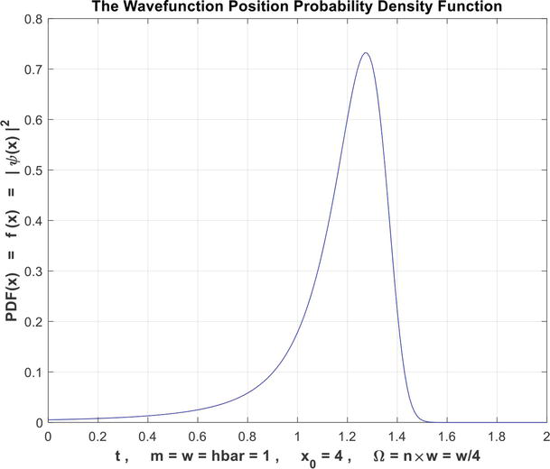
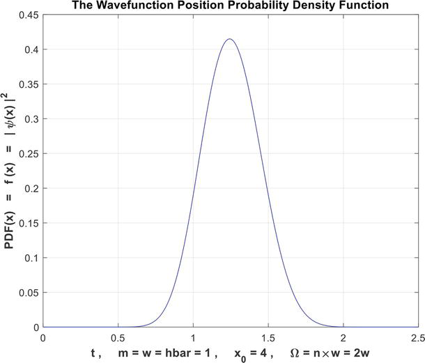
Figure 3.

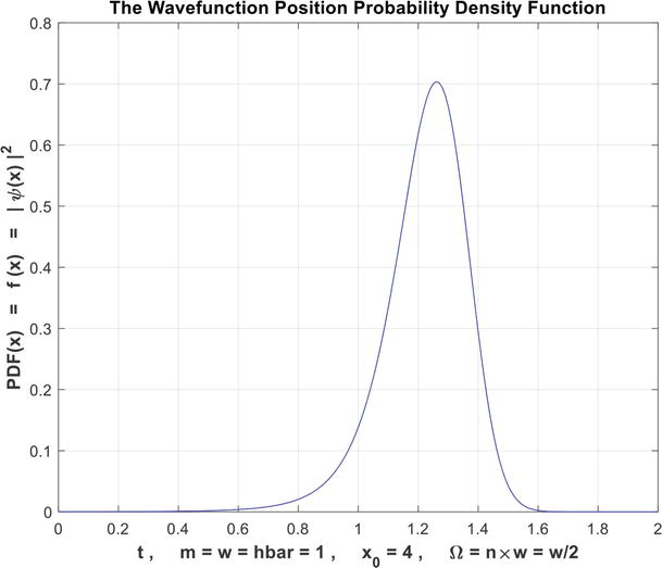
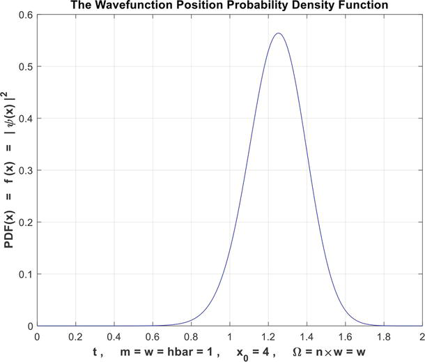
The graph of the PDF as a function of the random variable T of the wavefunction position probability density for n = 1/4.

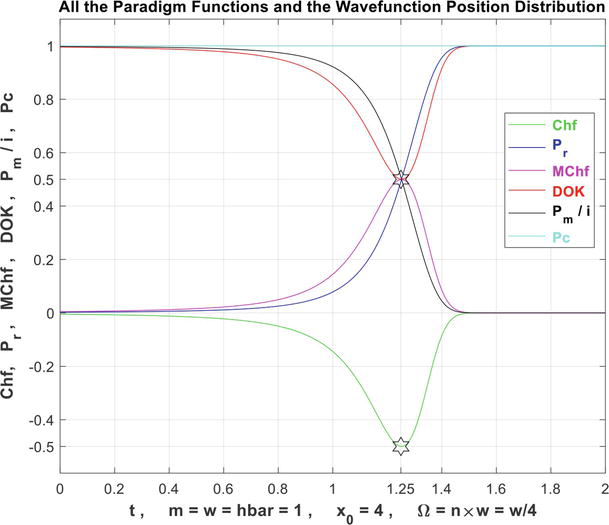
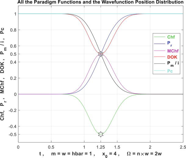
Figure 4.

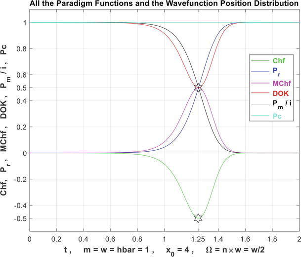
The graphs of all the CPP parameters for the wavefunction position probability distribution as functions of the random variable T for n = 1/4.

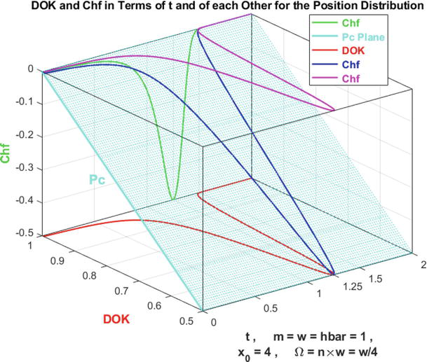
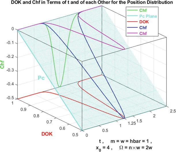
Figure 5.

The graphs of DOK and Chf and the deterministic probability Pc for the wavefunction position probability distribution in terms of T and of each other for n = 1/4.

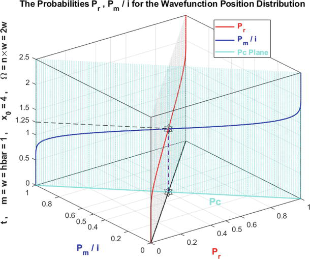
Figure 6.

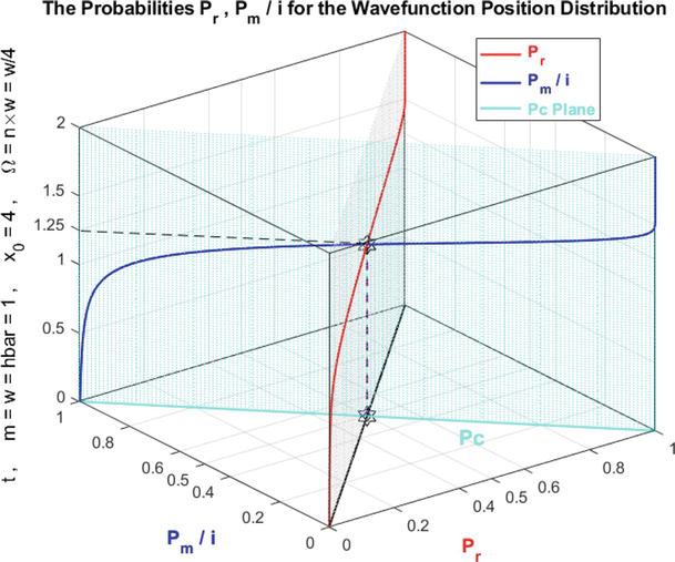
The graphs of P_r and P_m/i and Pc for the wavefunction position probability distribution in terms of T and of each other for n = 1/4.

Figure 7.

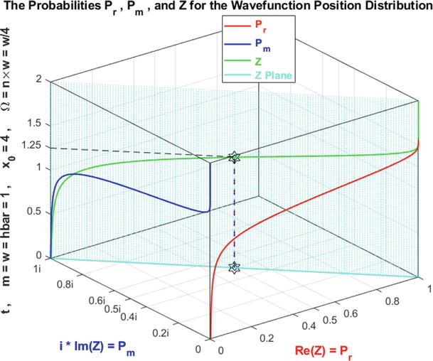
The graphs of the probabilities P_r and P_m and Z for the wavefunction position probability distribution in terms of T for n = 1/4.

Figure 8.

The graph of the PDF as a function of the random variable T of the wavefunction position probability density for n = 1/2.

Figure 9.

The graphs of all the CPP parameters for the wavefunction position probability distribution as functions of the random variable T for n = 1/2.

Figure 10.

The graphs of DOK and Chf and the deterministic probability Pc for the wavefunction position probability distribution in terms of T and of each other for n = 1/2.

Figure 11.

The graphs of P_r and P_m/i and Pc for the wavefunction position probability distribution in terms of T and of each other for n = 1/2.

Figure 12.

The graphs of the probabilities P_r and P_m and Z for the wavefunction position probability distribution in terms of T for n = 1/2.

Figure 13.

The graph of the PDF as a function of the random variable T of the wavefunction position probability density for n = 1.

Figure 14.

The graphs of all the CPP parameters for the wavefunction position probability distribution as functions of the random variable T for n = 1.

Figure 15.

The graphs of DOK and Chf and the deterministic probability Pc for the wavefunction position probability distribution in terms of T and of each other for n = 1.

Figure 16.

The graphs of P_r and P_m/i and Pc for the wavefunction position probability distribution in terms of T and of each other for n = 1.

Figure 17.

The graphs of the probabilities P_r and P_m and Z for the wavefunction position probability distribution in terms of T for n = 1.

Figure 18.

The graph of the PDF as a function of the random variable T of the wavefunction position probability density for n = 2.

Figure 19.

The graphs of all the CPP parameters for the wavefunction position probability distribution as functions of the random variable T for n = 2.

Figure 20.

The graphs of DOK and Chf and the deterministic probability Pc for the wavefunction position probability distribution in terms of T and of each other for n = 2.

Figure 21.

The graphs of P_r and P_m/i and Pc for the wavefunction position probability distribution in terms of T and of each other for n = 2.

Figure 22.

The graphs of the probabilities P_r and P_m and Z for the wavefunction position probability distribution in terms of T for n = 2.

Figure 23.

The graph of the PDF as a function of the random variable T of the wavefunction position probability density for n = 50.

Figure 24.

The graphs of all the CPP parameters for the wavefunction position probability distribution as functions of the random variable T for n = 50.

Figure 25.

The graphs of DOK and Chf and the deterministic probability Pc for the wavefunction position probability distribution in terms of T and of each other for n = 50.

Figure 26.

The graphs of P_r and P_m/i and Pc for the wavefunction position probability distribution in terms of T and of each other for n = 50.

Figure 27.

The graphs of the probabilities P_r and P_m and Z for the wavefunction position probability distribution in terms of T for n = 50.

Figure 28.

The graph of the PDF as a function of the random variable T of the wavefunction position probability density for n = 100.

Figure 29.

The graphs of all the CPP parameters for the wavefunction position probability distribution as functions of the random variable T for n = 100.

Figure 30.

The graphs of DOK and Chf and the deterministic probability Pc for the wavefunction position probability distribution in terms of T and of each other for n = 100.

Figure 31.

The graphs of P_r and P_m/i and Pc for the wavefunction position probability distribution in terms of T and of each other for n = 100.

Figure 32.

The graphs of the probabilities P_r and P_m and Z for the wavefunction position probability distribution in terms of T for n = 100.

Figure 33.

The graph of the PDF as a function of the random variable T of the wavefunction position probability density for n = 300.

Figure 34.

The graphs of all the CPP parameters for the wavefunction position probability distribution as functions of the random variable T for n = 300.

Figure 35.

The graphs of DOK and Chf and the deterministic probability Pc for the wavefunction position probability distribution in terms of T and of each other for n = 300.

Figure 36.

The graphs of P_r and P_m/i and Pc for the wavefunction position probability distribution in terms of T and of each other for n = 300.

Figure 37.

The graphs of the probabilities P_r and P_m and Z for the wavefunction position probability distribution in terms of T for n = 300.

4.3.1 Simulations interpretation

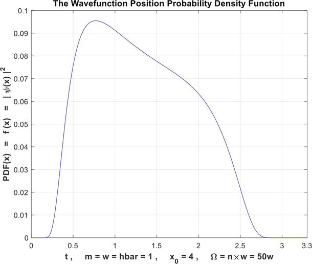
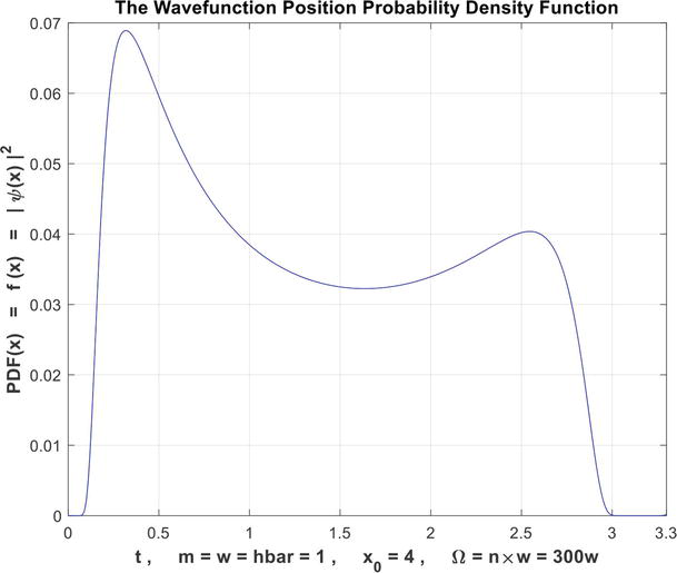
In Figures 3, 8, 13, 18, 23, 28, and 33, we can see the graphs of the probability density functions (PDF) of the wavefunction position probability distribution for this problem as functions of the time random variable $T:0\le T\le 3.3$ for n = 1/4, 1/2, 1, 2, 50, 100, and 300.

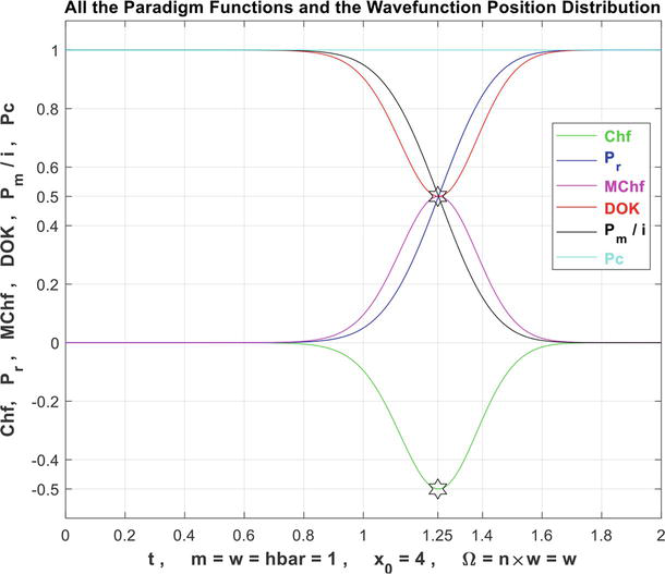
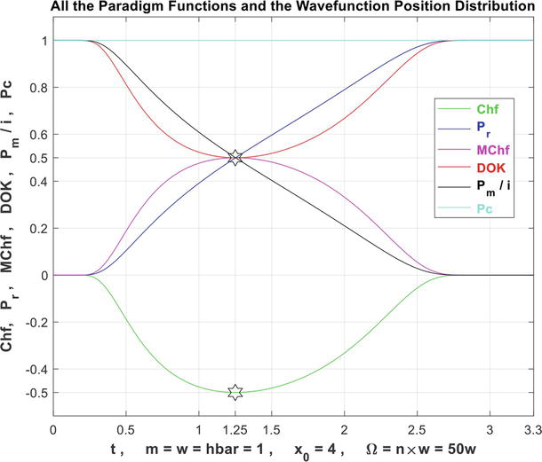
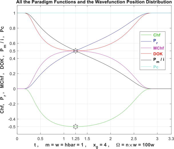
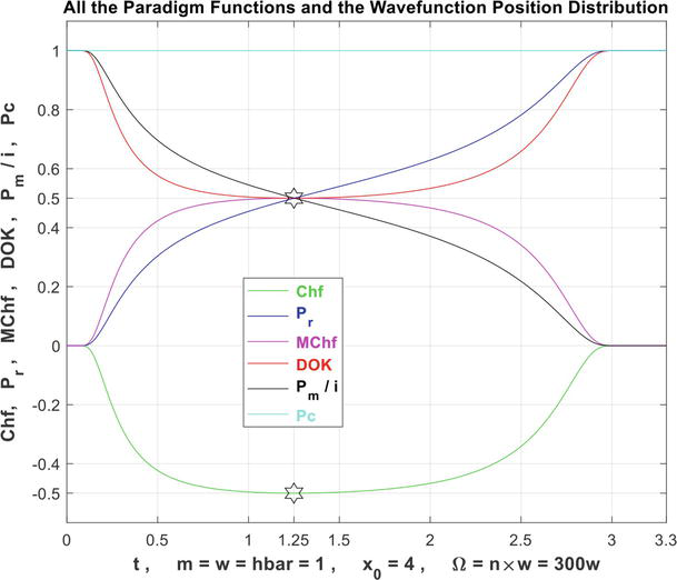
In Figures 4, 9, 14, 19, 24, 29, and 34, we can also see the graphs and the simulations of all the CPP parameters (Chf, MChf, DOK, P_r, P_m/i, and Pc) as functions of the time random variable T for the wavefunction position probability distribution of the quantum harmonic oscillators with Gaussian initial condition problem for n = 1/4, 1/2, 1, 2, 50, 100, and 300. Hence, we can visualize all the new paradigm functions for this problem.

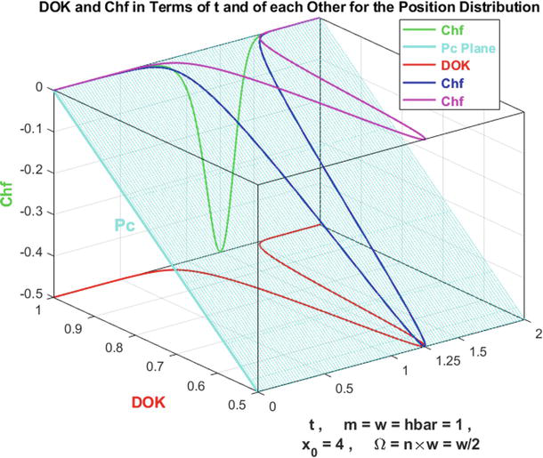
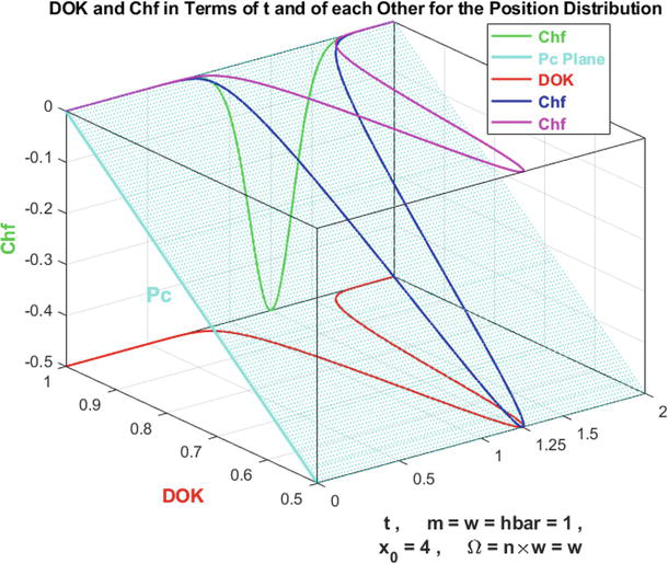
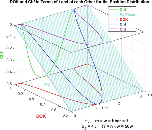
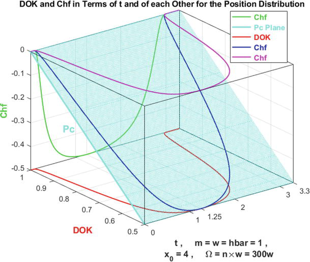
In the cubes (Figures 5, 10, 15, 20, 25, 30, and 35), the simulation of DOK and Chf as functions of each other and of the time random variable T for the quantum harmonic oscillators with Gaussian initial condition problem wavefunction position probability distribution can be seen. The thick line in cyan is the projection of the plane Pc²(T) = DOK(T) – Chf(T) = 1 = Pc(T) on the plane T = L_b = lower bound of T = 0. This thick line starts at the point (DOK = 1, Chf = 0) when T = L_b = 0, reaches the point (DOK = 0.5, Chf = –0.5) when T = 1.25, and returns at the end to (DOK = 1, Chf = 0) when T = U_b = upper bound of T. The other curves are the graphs of DOK(T) (red) and Chf(T) (green, blue, pink) in different simulation planes. Notice that they all have a minimum at the point (DOK = 0.5, Chf = –0.5, T = 0). The last simulation point corresponds to (DOK = 1, Chf = 0, T = U_b).

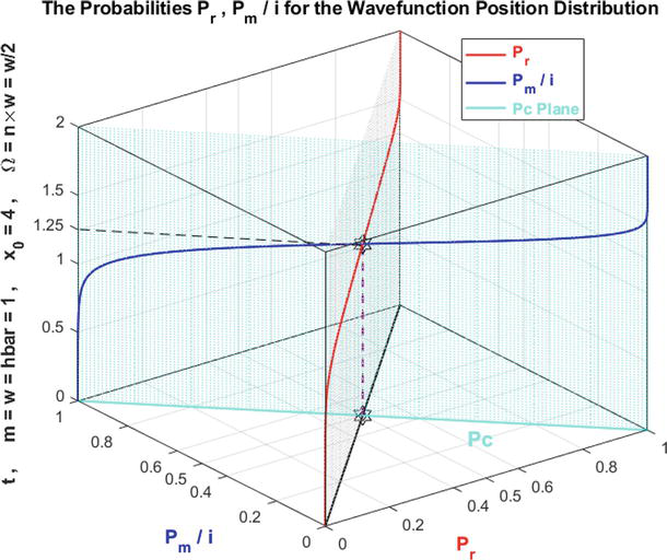
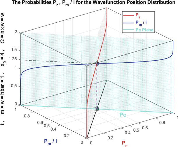
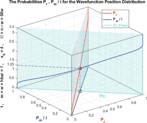
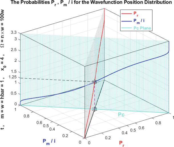
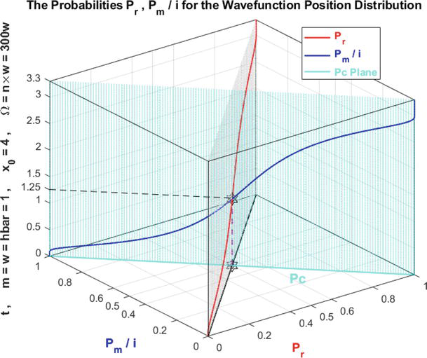
In the cubes (Figures 6, 11, 16, 21, 26, 31, and 36), we can notice the simulation of the real probability P_r(T) in $\mathcal{R}$ and its complementary real probability P_m(T)/i in $\mathcal{R}$ also in terms of the time random variable T for the quantum harmonic oscillators with Gaussian initial condition problem wavefunction position probability distribution. The thick line in cyan is the projection of the plane Pc²(T) = P_r(T) + P_m(T)/i = 1 = Pc(T) on the plane T = L_b = lower bound of T = 0. This thick line starts at the point (P_r = 0, P_m/i = 1) and ends at the point (P_r = 1, P_m/i = 0). The red curve represents P_r(T) in the plane P_r(T) = P_m(T)/i in light gray. This curve starts at the point (P_r = 0, P_m/i = 1, T = L_b = lower bound of T = 0), reaches the point (P_r = 0.5, P_m/i = 0.5, T = 1.25), and gets at the end to (P_r = 1, P_m/i = 0, T = U_b = upper bound of T). The blue curve represents P_m(T)/i in the plane in cyan P_r(T) + P_m(T)/i = 1 = Pc(T). Notice the importance of the point, which is the intersection of the red and blue curves at T = 1.25 and when P_r(T) = P_m(T)/i = 0.5.

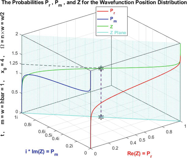
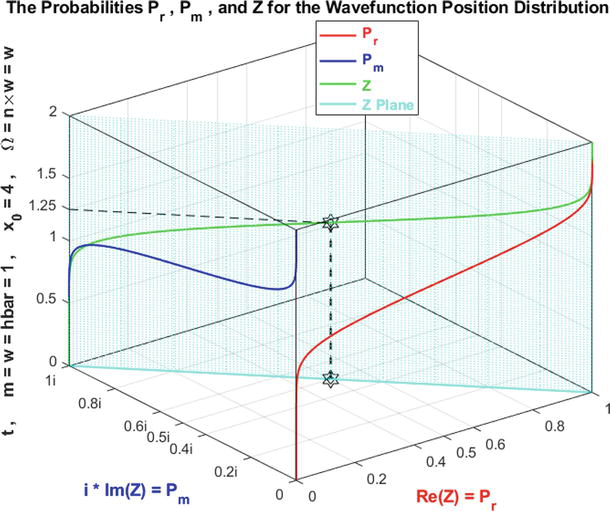
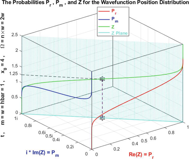
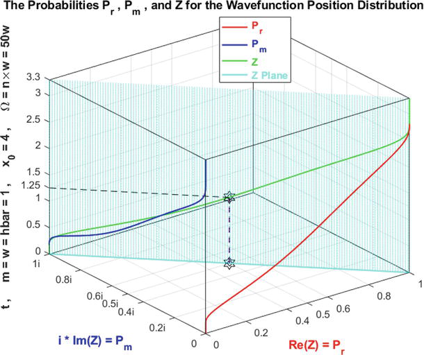
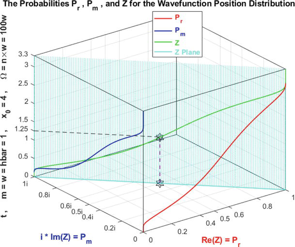
In the cubes (Figures 7, 12, 17, 22, 27, 32, and 37), we can notice the simulation of the complex probability Z(T) in $\mathcal{C}=\mathcal{R}+\mathcal{M}$ as a function of the real probability P_r(T) = Re(Z) in $\mathcal{R}$ and of its complementary imaginary probability P_m(T) = i×Im(Z) in $\mathcal{M}$, and this in terms of the time random variable T for the quantum harmonic oscillators with Gaussian initial condition problem wavefunction position probability distribution. The red curve represents P_r(T) in the plane P_m(T) = 0, and the blue curve represents P_m(T) in the plane P_r(T) = 0. The green curve represents the complex probability Z(T) = P_r(T) + P_m(T) = Re(Z) + i×Im(Z) in the plane P_r(T) = iP_m(T) + 1 or Z(T) plane in cyan. The curve of Z(T) starts at the point (P_r = 0, P_m= i, T = L_b = lower bound of T = 0) and ends at the point (P_r = 1, P_m = 0, T = U_b = upper bound of T). The thick line in cyan is P_r(T = L_b = 0) = iP_m(T = L_b = 0) + 1, and it is the projection of the Z(T) curve on the complex probability plane whose equation is: T = L_b = 0. This projected thick line starts at the point (P_r = 0, P_m= i, T = L_b = 0) and ends at the point (P_r = 1, P_m = 0, T = L_b = 0). Notice the importance of the point corresponding to T = 1.25 and Z = 0.5 + 0.5i when P_r = 0.5 and P_m = 0.5i.

4.4 The characteristics of the position probability distribution

In this quantum mechanics problem, the average, or expectation value of the position of a particle is given by Ref. [20]:

$$⟨x⟩=\underset{0}{\overset{+\infty }{\int }}t{\left|\psi \left(x,t\right)\right|}^2\mathit{dt}=\underset{0}{\overset{+\infty }{\int }}t\mathbb{N}\left(x_{0}cos\left(\mathit{wt}\right),\sqrt{\frac{\mathrm{\hslash }}{2m\mathrm{\Omega }}\left({cos}^2\left(\mathit{wt}\right)+\frac{{\mathrm{\Omega }}^2}{w^2}{sin}^2\left(\mathit{wt}\right)\right)}\right)\mathit{dt}$$E21

For this problem, it can be shown that the average position is always $⟨x⟩=x_{0}cos\left(\mathit{wt}\right)$.

So, in the probability set and universe $\mathcal{R}$, we have:

$${⟨x⟩}_R=⟨x⟩=x_{0}cos\left(\mathit{wt}\right)$$E22

The variance in the position is a measure of the uncertainty in the position of the particle, so in the probability set and universe $\mathcal{R}$, we have:

$$\begin{array}{l}{\mathrm{Var}}_{x,R}=\mathrm{Var}\left(x\right)={⟨x^2⟩}_R-{⟨x⟩}_R^2\\ =\left\{\underset{0}{\overset{+\infty }{\int }}{t}^2{\left|\psi \left(x,t\right)\right|}^2\mathit{dt}\right\}-{\left\{\underset{0}{\overset{+\infty }{\int }}t{\left|\psi \left(x,t\right)\right|}^2\mathit{dt}\right\}}^2\end{array}$$

$$\begin{array}{l}=\left\{\underset{0}{\overset{+\infty }{\int }}{t}^2\mathbb{N}\left(x_{0}cos\left(\mathit{wt}\right),\sqrt{\frac{\mathrm{\hslash }}{2m\mathrm{\Omega }}\left({cos}^2\left(\mathit{wt}\right)+\frac{{\mathrm{\Omega }}^2}{w^2}{sin}^2\left(\mathit{wt}\right)\right)}\right)\mathit{dt}\right\}-{\left[x_{0}cos\left(\mathit{wt}\right)\right]}^2\\ =\frac{\mathrm{\hslash }}{2m\mathrm{\Omega }}\left({cos}^2\left(\mathit{wt}\right)+\frac{{\mathrm{\Omega }}^2}{w^2}{sin}^2\left(\mathit{wt}\right)\right)\end{array}$$E23

In the probability set and universe $\mathcal{M}$, we have:

$$\begin{array}{rcl}{⟨x⟩}_M& =& \underset{0}{\overset{+\infty }{\int }}t\left\{i\left[1-{\left|\psi \left(x,t\right)\right|}^2\right]\right\}\mathit{dt}\\ & =& i\underset{0}{\overset{+\infty }{\int }}t\left\{1-\mathbb{N}\left(x_{0}cos\left(\mathit{wt}\right),\sqrt{\frac{\mathrm{\hslash }}{2m\mathrm{\Omega }}\left({cos}^2\left(\mathit{wt}\right)+\frac{{\mathrm{\Omega }}^2}{w^2}{sin}^2\left(\mathit{wt}\right)\right)}\right)\right\}\mathit{dt}\\ & =& i\left\{\underset{0}{\overset{U_b}{\int }}\mathit{tdt}-\underset{0}{\overset{+\infty }{\int }}t\mathbb{N}\left(x_{0}cos\left(\mathit{wt}\right),\sqrt{\frac{\mathrm{\hslash }}{2m\mathrm{\Omega }}\left({cos}^2\left(\mathit{wt}\right)+\frac{{\mathrm{\Omega }}^2}{w^2}{sin}^2\left(\mathit{wt}\right)\right)}\right)\mathit{dt}\right\}\\ & =& i\left\{{\left[\frac{t^2}{2}\right]}_0^{U_b}-{⟨x⟩}_R\right\}=i\left\{\frac{U_b^2}{2}-x_{0}cos\left(\mathit{wt}\right)\right\}\end{array}$$E24

where $U_b$ is the upper bound of the definite integral above. Practically, the standard normal distribution probability is very nearly equal to 1.0000 (0.99997 exactly) for $U_b=4$.

Note that, $\text{If}{U}_b\to +\infty \iff {⟨x⟩}_M\to +\infty$.

Moreover,

$$\begin{array}{rcl}{\mathrm{Var}}_{x,M}& =& {⟨x^2⟩}_M-{⟨x⟩}_M^2\\ & =& \left\{\underset{0}{\overset{+\infty }{\int }}{t}^2\left\{i\left[1-{\left|\psi \left(x,t\right)\right|}^2\right]\right\}\mathit{dt}\right\}-{\left\{\underset{0}{\overset{+\infty }{\int }}t\left\{i\left[1-{\left|\psi \left(x,t\right)\right|}^2\right]\right\}\mathit{dt}\right\}}^2\\ & =& i\underset{0}{\overset{+\infty }{\int }}{t}^2\left\{1-\mathbb{N}\left(x_{0}cos\left(\mathit{wt}\right),\sqrt{\frac{\mathrm{\hslash }}{2m\mathrm{\Omega }}\left({cos}^2\left(\mathit{wt}\right)+\frac{{\mathrm{\Omega }}^2}{w^2}{sin}^2\left(\mathit{wt}\right)\right)}\right)\right\}\mathit{dt}\\ & & -{\left\{i\left[\frac{U_b^2}{2}-x_{0}cos\left(\mathit{wt}\right)\right]\right\}}^2\end{array}$$

$$\begin{array}{l}=i\left\{\underset{0}{\overset{U_b}{\int }}{t}^2\mathit{dt}-\underset{0}{\overset{+\infty }{\int }}{t}^2\left\{\mathbb{N}\left(x_{0}cos\left(\mathit{wt}\right),\sqrt{\frac{\mathrm{\hslash }}{2m\mathrm{\Omega }}\left({cos}^2\left(\mathit{wt}\right)+\frac{{\mathrm{\Omega }}^2}{w^2}{sin}^2\left(\mathit{wt}\right)\right)}\right)\right\}\mathit{dt}\right\}+{\left[\frac{U_b^2}{2}-x_{0}cos\left(\mathit{wt}\right)\right]}^2\\ =i\left\{\underset{0}{\overset{U_b}{\int }}{t}^2\mathit{dt}-{\mathrm{Var}}_{x,R}\right\}+{\left[\frac{U_b^2}{2}-x_{0}cos\left(\mathit{wt}\right)\right]}^2=i\left\{{\left[\frac{t^3}{3}\right]}_0^{U_b}-{\mathrm{Var}}_{x,R}\right\}+{\left[\frac{U_b^2}{2}-x_{0}cos\left(\mathit{wt}\right)\right]}^2\\ =i\left\{\frac{U_b^3}{3}-\frac{\mathrm{\hslash }}{2m\mathrm{\Omega }}\left({cos}^2\left(\mathit{wt}\right)+\frac{{\mathrm{\Omega }}^2}{w^2}{sin}^2\left(\mathit{wt}\right)\right)\right\}+{\left[\frac{U_b^2}{2}-x_{0}cos\left(\mathit{wt}\right)\right]}^2\end{array}$$E25

Note that, $\text{if}{U}_b\to +\infty \iff {\mathrm{Var}}_{x,M}\to +\infty$.

In the probability set and the universe $\mathcal{C}=\mathcal{R}+\mathcal{M}$, we have from CPP:

$${⟨x⟩}_C=\underset{0}{\overset{+\infty }{\int }}t\left[z\left(x,t\right)\right]\mathit{dt}=\underset{0}{\overset{+\infty }{\int }}t\left\{{\left|\psi \left(x,t\right)\right|}^2+i\left[1-{\left|\psi \left(x,t\right)\right|}^2\right]\right\}\mathit{dt}$$

$$\begin{array}{l}=\underset{0}{\overset{+\infty }{\int }}t{\left|\psi \left(x,t\right)\right|}^2\mathit{dt}+\underset{0}{\overset{+\infty }{\int }}t\left\{i\left[1-{\left|\psi \left(x,t\right)\right|}^2\right]\right\}\mathit{dt}\\ =\underset{0}{\overset{+\infty }{\int }}t\mathbb{N}\left(x_{0}cos\left(\mathit{wt}\right),\sqrt{\frac{\mathrm{\hslash }}{2m\mathrm{\Omega }}\left({cos}^2\left(\mathit{wt}\right)+\frac{{\mathrm{\Omega }}^2}{w^2}{sin}^2\left(\mathit{wt}\right)\right)}\right)\mathit{dt}\\ +i\underset{0}{\overset{+\infty }{\int }}t\left\{1-\mathbb{N}\left(x_{0}cos\left(\mathit{wt}\right),\sqrt{\frac{\mathrm{\hslash }}{2m\mathrm{\Omega }}\left({cos}^2\left(\mathit{wt}\right)+\frac{{\mathrm{\Omega }}^2}{w^2}{sin}^2\left(\mathit{wt}\right)\right)}\right)\right\}\mathit{dt}\\ ={⟨x⟩}_R+{⟨x⟩}_M=x_{0}cos\left(\mathit{wt}\right)+i\left\{\frac{U_b^2}{2}-x_{0}cos\left(\mathit{wt}\right)\right\}\end{array}$$E26

Note that, $\text{If}{U}_b\to +\infty \iff {⟨x⟩}_C\to +\infty$.

$$\begin{array}{rcl}{\mathrm{Var}}_{x,C}& =& {⟨x^2⟩}_C-{⟨x⟩}_C^2=\left[\underset{0}{\overset{+\infty }{\int }}{t}^2\left[z\left(x,t\right)\right]\mathit{dt}\right]-{\left[{⟨x⟩}_R+{⟨x⟩}_M\right]}^2\\ & =& \left[\underset{0}{\overset{+\infty }{\int }}{t}^2\left\{{\left|\psi \left(x,t\right)\right|}^2+i\left[1-{\left|\psi \left(x,t\right)\right|}^2\right]\right\}\mathit{dt}\right]-{\left[{⟨x⟩}_R+{⟨x⟩}_M\right]}^2\\ & =& \left[\underset{0}{\overset{+\infty }{\int }}{t}^2{\left|\psi \left(x,t\right)\right|}^2\mathit{dt}+\underset{0}{\overset{+\infty }{\int }}{t}^2\left\{i\left[1-{\left|\psi \left(x,t\right)\right|}^2\right]\right\}\mathit{dt}\right]-{\left[{⟨x⟩}_R+{⟨x⟩}_M\right]}^2\\ & =& \left[{⟨x^2⟩}_R+{⟨x^2⟩}_M\right]-{\left[{⟨x⟩}_R+{⟨x⟩}_M\right]}^2\\ & =& \left[{⟨x^2⟩}_R+{⟨x^2⟩}_M\right]-\left[{⟨x⟩}_R^2+{⟨x⟩}_M^2+2{⟨x⟩}_R{⟨x⟩}_M\right]\\ & =& \left[{⟨x^2⟩}_R-{⟨x⟩}_R^2\right]+\left[{⟨x^2⟩}_M-{⟨x⟩}_M^2\right]-2{⟨x⟩}_R{⟨x⟩}_M\\ & =& {\mathrm{Var}}_{x,R}+{\mathrm{Var}}_{x,M}-2{⟨x⟩}_R{⟨x⟩}_M\\ & =& \frac{\mathrm{\hslash }}{2m\mathrm{\Omega }}\left({cos}^2\left(\mathit{wt}\right)+\frac{{\mathrm{\Omega }}^2}{w^2}{sin}^2\left(\mathit{wt}\right)\right)+i\left\{\frac{U_b^3}{3}-\frac{\mathrm{\hslash }}{2m\mathrm{\Omega }}\left({cos}^2\left(\mathit{wt}\right)+\frac{{\mathrm{\Omega }}^2}{w^2}{sin}^2\left(\mathit{wt}\right)\right)\right\}\\ & & +{\left[\frac{U_b^2}{2}-x_{0}cos\left(\mathit{wt}\right)\right]}^2-2\left\{x_{0}cos\left(\mathit{wt}\right)\right\}\times \left\{i\left\{\frac{U_b^2}{2}-x_{0}cos\left(\mathit{wt}\right)\right\}\right\}\end{array}$$E27

Note that, $\text{If}{U}_b\to +\infty \iff {\mathrm{Var}}_{x,C}\to +\infty$.

Tables 1–4 compute the position distribution characteristics for $x_0=4$, $m=w=\mathrm{\hslash }=1$, $n=1/4$ where $\mathrm{\Omega }=n\times w$, and $U_b=4,20,50,1000$.

Position distribution characteristics	$x_0=4$, $m=w=\mathrm{\hslash }=1$, $\mathrm{\Omega }=w/4$, $U_b=4$
${⟨x⟩}_R$	$-2.6146$
${\mathrm{Var}}_{x,R}$	0.9261
${⟨x⟩}_M$	i×10.6146
${\mathrm{Var}}_{x,M}$	112.6692+i×20.4072
${⟨x⟩}_C={⟨x⟩}_R+{⟨x⟩}_M$	$-2.6146$+i×10.6146
${\mathrm{Var}}_{x,C}={\mathrm{Var}}_{x,R}+{\mathrm{Var}}_{x,M}-2{⟨x⟩}_R{⟨x⟩}_M$	113.5953+i×75.9124

Table 1.

The position distribution characteristics for $U_b=4$ and $n=1/4$_.

Position distribution characteristics	$x_0=4$, $m=w=\mathrm{\hslash }=1$, $\mathrm{\Omega }=w/4$, $U_b=20$
${⟨x⟩}_R$	1.6323
${\mathrm{Var}}_{x,R}$	0.4372
${⟨x⟩}_M$	i×198.3677
${\mathrm{Var}}_{x,M}$	3.9350e+04+i×2.6662e+03
${⟨x⟩}_C={⟨x⟩}_R+{⟨x⟩}_M$	1.6323+i×198.3677
${\mathrm{Var}}_{x,C}={\mathrm{Var}}_{x,R}+{\mathrm{Var}}_{x,M}-2{⟨x⟩}_R{⟨x⟩}_M$	3.9350e+04+i×2.0186e+03

Table 2.

The position distribution characteristics for $U_b=20$ and $n=1/4$_.

Position distribution characteristics	$x_0=4$, $m=w=\mathrm{\hslash }=1$, $\mathrm{\Omega }=w/4$, $U_b=50$
${⟨x⟩}_R$	3.8599
${\mathrm{Var}}_{x,R}$	1.8709
${⟨x⟩}_M$	i×1.2461e+03
${\mathrm{Var}}_{x,M}$	1.5529e+06+i×4.1665e+04
${⟨x⟩}_C={⟨x⟩}_R+{⟨x⟩}_M$	3.8599+ i×1.2461e+03
${\mathrm{Var}}_{x,C}={\mathrm{Var}}_{x,R}+{\mathrm{Var}}_{x,M}-2{⟨x⟩}_R{⟨x⟩}_M$	1.5529e+06+i×3.2045e+04

Table 3.

The position distribution characteristics for $U_b=50$ and $n=1/4$.

Position distribution characteristics	$x_0=4$, $m=w=\mathrm{\hslash }=1$, $\mathrm{\Omega }=w/4$, $U_b=1000$
${⟨x⟩}_R$	2.2495
${\mathrm{Var}}_{x,R}$	0.7180
${⟨x⟩}_M$	i×5.0000e+05
${\mathrm{Var}}_{x,M}$	2.5000e+11+i×3.3333e+08
${⟨x⟩}_C={⟨x⟩}_R+{⟨x⟩}_M$	2.2495+ i×5.0000e+05
${\mathrm{Var}}_{x,C}={\mathrm{Var}}_{x,R}+{\mathrm{Var}}_{x,M}-2{⟨x⟩}_R{⟨x⟩}_M$	2.5000e+11+i×3.3108e+08

Table 4.

The position distribution characteristics for $U_b=1000$ and $n=1/4$.

5. Conclusion and perspectives

In the present research chapter, the novel extended system of eight axioms (EKA) of A. N. Kolmogorov was applied and linked to the quantum harmonic oscillators with the Gaussian initial condition problem in quantum mechanics theory. Thus, a strong bond between quantum mechanics and the novel paradigm (CPP) was accomplished. Hence, the Paradigm of “Complex Probability” was more elaborated beyond the scope of my 23 previous research publications on this topic.

Furthermore, as it was verified and proved in the original paradigm, before the beginning of the simulation of the random event and at its end we have the chaotic factor (Chf and MChf) is 0 and the degree of our knowledge (DOK) is 1 since the stochastic and probabilistic effects and fluctuations have either not started yet or they have finished and terminated their task on the random phenomenon. During the execution of the nondeterministic experiment and process we also have: –0.5 ≤ Chf < 0, 0 < MChf ≤ 0.5, and 0.5 ≤ DOK < 1. We can see that during the whole process, we have constantly and incessantly ${\mathit{Pc}}^2=\mathit{DOK}-\mathit{Chf}=\mathit{DOK}+\mathit{\text{MChf}}=1=\mathit{Pc}$, that shows that the simulation which behaved probabilistically and randomly in the real universe and set $\mathcal{R}$ is now deterministic and certain in the complex probability universe and set $\mathcal{C}=\mathcal{R}+\mathcal{M}$, and this after adding to the stochastic phenomenon performed in the real universe and set $\mathcal{R}$ the contributions of the imaginary universe and set $\mathcal{M}$ and thus after subtracting and eliminating from the degree of our knowledge the chaotic factor.

This is certainly very wonderful, fascinating, and fruitful and shows and proves once again the rewards of extending the five axioms of the probability of A. N. Kolmogorov and thus the benefits and novelty of my original and novel model in the fields of applied mathematics, prognostics, and quantum mechanics that can be called verily: “The Complex Probability Paradigm.” As future and prospective challenges and research works, we intend to elaborate more on the original probability paradigm developed and to apply it to a large array of stochastic phenomena and nondeterministic experiments encountered in the theory of quantum mechanics.

Conflicts of interest

The author declares that there are no conflicts of interest regarding the publication of this research work.

Data availability

The data used to support the findings of this study are available from the author upon request.

Nomenclature

$\mathcal{R}$

probabilities and events real set

$\mathcal{M}$

probabilities and events imaginary set

$\mathcal{C}$

probabilities and events complex set

i

the imaginary number where $i^2=-1$ or $i=\sqrt{-1}$

EKA

Extended Kolmogorov’s Axioms

CPP

Complex Probability Paradigm

P_rob

any event probability

P_r

probability of an event in the real set $\mathcal{R}$

P_m

probability of an event in the imaginary set $\mathcal{M}$ associated with the real probability in $\mathcal{R}$

Pc

probability of an event in $\mathcal{R}$ with its corresponding complementary event in $\mathcal{M}$= probability in the complex probability set $\mathcal{C}=\mathcal{R}+\mathcal{M}$

Z

complex probability number = sum of P_r and P_m = complex random vector

DOK = ${\left|Z\right|}^2$

the random experiment or system degree of our knowledge; it is the square of the norm of Z

Chf

the chaotic factor of Z

MChf

the magnitude of the chaotic factor of Z

${\left|\psi \left(x,t\right)\right|}^2$

probability density function of the position wavefunction

${\left|\varphi \left(p,t\right)\right|}^2$

probability density function of the momentum wavefunction

${⟨x⟩}_R$,${⟨x⟩}_M$,${⟨x⟩}_C$

averages, or expectations, or means of the position wavefunction probability density function in $\mathcal{R}$, $\mathcal{M}$, and $\mathcal{C},$ respectively

${\mathrm{Var}}_{x,R}$,${\mathrm{Var}}_{x,M}$,${\mathrm{Var}}_{x,C}$

variances of the position wavefunction probability density function in $\mathcal{R}$, $\mathcal{M}$, and $\mathcal{C},$respectively

${⟨p⟩}_R$,${⟨p⟩}_M$,${⟨p⟩}_C$

averages, or expectations, or means of the momentum wavefunction probability density function in $\mathcal{R}$, $\mathcal{M}$, and $\mathcal{C},$ respectively

${\mathrm{Var}}_{p,R}$,${\mathrm{Var}}_{p,M}$,${\mathrm{Var}}_{p,C}$

variances of the momentum wavefunction probability density function in $\mathcal{R}$, $\mathcal{M}$, and $\mathcal{C},$ respectively

$H_x^R$

entropy in the real universe $\mathcal{R}$ of the particle position

${\mathit{\text{NegH}}}_x^R$

negative entropy in the real universe $\mathcal{R}$ of the particle position

${\overline{H}}_x^R$

complementary entropy in the real universe $\mathcal{R}$ of the particle position

$H_x^M$

entropy in the imaginary universe $\mathcal{M}$ of the particle position

$H_x^C$

entropy in the complex universe $\mathcal{C}$ of the particle position

$H_p^R$

entropy in the real universe $\mathcal{R}$ of the particle momentum

${\mathit{\text{NegH}}}_p^R$

negative entropy in the real universe $\mathcal{R}$ of the particle momentum

${\overline{H}}_p^R$

complementary entropy in the real universe $\mathcal{R}$ of the particle momentum

$H_p^M$

entropy in the imaginary universe $\mathcal{M}$ of the particle momentum

$H_p^C$

entropy in the complex universe $\mathcal{C}$ of the particle momentum