Perspective Chapter: Mix-Unmix Pan-Sharpener – Novel Pan-Sharpening Method Based on Mixing Constituent Multispectral Bands and Unmixing Panchromatic Band

Abstract

A panchromatic band (Pan-band) spectrally covers a number of the other bands (multispectral-bands, MS). The Pan-band is of higher spatial resolution than the MS. The respective advantages of the two are combined through pan-sharpening with the resultant image adopting the higher spatial resolution of the Pan-band and the colour information of the MS. Various techniques have evolved but most of them cannot pan-sharpen more than three MS, and none of them can pan-sharpen more than three MS at a go, nor pan-sharpen a multispectral image not geographically covered by the Pan-band. This novel concept overcomes the first problem. The sequel to this chapter will address the second problem through reverse pan-sharpening. The concept argues that for a given pixel in the Pan-band, the strata of digital numbers (DNs) in the MS combine to give rise to a panchromatic-DN. The concept estimates respective coefficients of strata of DNs in the encompassed bands corresponding to pure blocks of pixels in the Pan-band. On the basis of the coefficients, encompassed bands’ DN contributions to the panchromatic-DN are computed from the Pan-band DN. The resultant DN contributions are regressed on the MS-DNs and one of the encompassed MS pan-sharpened on the basis of its model. The other multi-spectral bands are pan-sharpened through it.

1. Introduction

All Earth observation satellites are multi-band. In most cases, there is a band that collectively covers some of the other bands. The band covering the collective spectral ranges covered by individual bands is called the panchromatic band. The other bands are collectively referred to as multi-spectral bands. The panchromatic band always has a higher spatial resolution than the multispectral bands it encompasses. For instance, for Geoeye-1, the panchromatic band covers the spectral range 450 nm–800 nm encompassing the blue (450 nm–510 nm), green (510 nm–580 nm), red (655 nm–690 nm), and partially near-infra red (780 nm–920 nm) bands. The spatial resolution of the panchromatic band is 0.41 m against 1.65 m for the multi-spectral bands.

A panchromatic band does not provide colour information as it cannot be viewed in combination with the other bands due to differing spatial resolution. The encompassed multispectral bands when viewed in combination, made possible by a common spatial resolution, provide colour information in the RGB colour space through colour combination. However, due to the higher spatial resolution, the panchromatic band provides greater spatial detail than the multispectral bands. For a variety of applications, an image with both high spatial and spectral resolutions would be desirable. The higher spatial detail of the panchromatic band and colour information of the multispectral bands can be combined through the process of image fusion by pan-sharpening [1], defined pan-sharpening as fusion of a multi-spectral image and panchromatic data aimed at generating an outcome with the same spatial resolution of the panchromatic data and the spectral resolution of the multispectral image [2], defined it as merging the spatial and spectral information of the source images into a fused one, which has a higher spatial and spectral resolution and is more reliable for downstream tasks compared with any of the source images.

Pan-sharpening may also be across multispectral imagery [3, 4], discussed fusion of hyperspectral and multispectral imagery, noting that: the latter has detailed spectral information for fine classification and identification of land-cover but the narrow bandwidths limit absorption of reflected surface energy; the former has limited representation of spectral information making it difficult to characterise the spectral features but the higher spatial resolution allows for more complete description of the morphology and distribution of land-cover. Fusion of the two provides high spatial resolution and detailed spectral information for value-addition to remotely sensed data.

There have been numerous studies on pan-sharpening and development of pan-sharpening algorithms with the aim of preserving spectral information while increasing the spatial resolution of low-resolution multispectral data. However, there seems to be no universal categorisation criteria of pan-sharpening techniques. For instance [1], categorises the techniques into (i) Component substitution, (ii) Multi-resolution analysis, and (iii) third generation techniques e.g. variational optimization and machine learning techniques; [2] has (i) Component substitution, (ii) Multi-resolution analysis, (iii) Degradation model, (iv) Deep neural network; [5] has (i) Component substitution-, (ii) Relative spectral contribution-, (iii) High-frequency injection-, (iv) Methods based on the statistics of the image-, (v) Multiresolution-family. Despite the disharmony, two classical techniques are common to all reviewers: component substitution and multi-resolution analysis. [6, 7, 8, 9, 10, 11, 12] give further detailed discussions on pan-sharpening techniques.

2. Classical pan-sharpening techniques

A need arises to harmonise the criteria for categorisation of pan-sharpening techniques. This chapter cannot cover all the uttered categories of pan-sharpening techniques.

2.1 Component substitution techniques

Component Substitution (CS) techniques include among others, The Brovey transform, Intensity-Hue-Saturation (IHS) and Principal Component Analysis (PCA) methods [13]. As a requirement for all the aforementioned methods, the images must be co-registered and resampled, the quality of which impacts on the results of pan-sharpening [13, 14]. The IHS method is the most popular of the three and involves conversion of a three-band image from the RGB colour space to the IHS colour space [15]. However, the technique has been shown to produce fused images with spectral and colour distortions [15, 16]. Modifications to the IHS method have included extension from three bands to four bands with the inclusion of near-infrared and the incorporation of weighting coefficients on the green and blue bands to minimise the difference between I and the panchromatic band [17]. Recent studies and developments have led to the development of other CS-based techniques and algorithms including the Fast Spectral Response Function (FSRF), the GIHS with Genetic Algorithm (GIHS-GA), the GIHS with Trade-off Parameter (GIHS-TP), University of New Brunswick (UNB)-Pan-sharpen and the Weighted Sum Image Sharpening (WSIS) techniques [16]. The aforementioned methods were evaluated using a uniform data set in the 2006 GRS-S Data-Fusion contest and were generally found to have various shortcomings including poor colour synthesis, missing colours and features, and blurred contours and shapes [16].

2.2 Multiresolution analysis techniques (MRA)

MRA methods, also referred to as wavelet-based fusion methods, include but are not limited to Generalised Laplacian Pyramid (GLP), Discrete Wavelet Transform (DWT), Contour-let transform, and Additive Wavelets Luminance Proportional (AWLP) techniques [6, 18]. These techniques employ the basic principle of extraction of spatial detail information from the high-resolution panchromatic image, which is not present in the low-resolution multispectral images and injecting it into the latter [6]. These methods preserve spectral characteristics of the multispectral image better than CS methods but tend to have less spatial information [15, 18].

Thus, depending on the application, it seems the trade-off is between the preservation of spectral information with limited increase in spatial resolution and distorted spectral information with increasing spatial resolution. Hybrid techniques aim to overcome the limitations of the CS- and MRA-based techniques, to preserve the spectral and spatial information content of the input images [16].

3. Materials and methods

This chapter introduces a novel pan-sharpening technique, the mix-unmix pan-sharpener, based on the Mix-unmix Classifier [19, 20]. The classifier was developed to overcome the problem of under-determinacy in linear spectral unmixing. Optical panchromatic and multispectral imagery are utilised in demonstration of the Mix-unmix Pan-sharpener.

3.1 Theory of the mix-unmix pan-sharpener

For a given sensor, a panchromatic band covers a number of multi-spectral bands. The former has a higher spatial resolution than the latter. One multispectral pixel covers an area of n x n (where n is at least 2) panchromatic pixels. If the n x n panchromatic pixels have the same DN, then the geographically corresponding multispectral pixel, ignoring any radiometric errors, can be taken to be spectrally pure. For instance, the panchromatic Band 8 (wavelength range = 0.50 nm–0.90 nm) of Landsat ETM+ has a spatial resolution of 14.25 m and spectrally covers the first four bands (spatial resolution of 28.5 m), namely: blue (0.45 nm–0.52 nm), green (0.52 nm–0.60 nm), red (0.63 nm–0.69 nm), and near-infra-red (0.76 nm–0.90 nm) of the sensor. This implies that the panchromatic band can be taken to be a mixture of reflectance from the other four bands. Therefore, it can be hypothesised that for a given pixel, the panchromatic DN can be decomposed into four multispectral DNs. In other words, the four multi-spectral DNs for the pixel mix result in the panchromatic DN. This begs the question: in what ratio do the four multispectral DNs mix to give rise to the panchromatic DN?

3.2 Study area, data, and determination of pure multispectral pixels

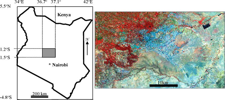
The study area is located in Kenya and Landsat ETM+ data is utilised for the research (Figure 1). The Mix-unmix pan-sharpener moves a 2×2 kernel over the panchromatic Band 8 and if all the four DNs in the kernel are the same, the value and also the multispectral DNs from bands one to four of the geographically corresponding pixels are retrieved. It is worth noting that the kernel does not cover any panchromatic pixel more than once nor does it skip any. The dimensions of the panchromatic band must be a multiple of n, and the band must, for this demonstration, geographically cover the multispectral bands. Table 1 is an extract of DNs of pure pixels.

Figure 1.

Location of the study area (left), and 28.5 m spatial resolution Landsat ETM+ image of the study area; RGB = 431. Dimensions in pixels: Y = 993, X = 1639.

No.	Band 8	Band 1	Band 2	Band 3	Band 4
1	21	59	40	29	16
2	21	61	40	28	16
3	23	62	44	34	16
4	28	68	54	42	19
….
909	95	99	98	149	102
910	98	106	112	148	103
911	98	134	131	160	79

Table 1.

DNs of pure blocks of pixels in the panchromatic band 8 and the corresponding multispectral DNs in bands 1 through 4. There are 911 such blocks comprising 59 (range 21–98) out of 192 different DNs (21–228).

3.3 Determination of the most probable mixing ratios

The approach adopted in determination of mixing ratios in this research borrows from [19, 20]. In developing the Mix-unmix Classifier, they mixed all the DNs of all possible end-members in all possible complementary combinations to synthesise all possible hypothetical mixed DNs. Through back-propagation, they determined the most probable abundances of the initial end-members. In this research, the multi-spectral bands one to four are synonymous with end-members, the multispectral DNs in Table 1 (columns two to four) are synonymous with the DNs of end-members and the corresponding panchromatic DN (column 1) is synonymous with the DN of a mixture of the end-members. The mix-unmix pan-sharpening involves four steps: (1) determination of all possible mixture ratios of the multispectral DNs associated with a panchromatic DN; (2) determination of universal mixture ratios of multispectral DNs for the given panchromatic DN; (3) decomposition of the panchromatic DN, and; (4) pan-sharpening all the multi-spectral bands.

3.3.1 Determination of all possible mixture ratios

For simplicity, this research assumes that the multispectral DNs (Table 1, columns two to four) mix in a linear manner to give rise to the respective panchromatic DN (Table 1, column two). This is modelled as follows:

$$D{N}_P=f_1.D{N}_1+f_2.D{N}_2+f_3.D{N}_3+f_4.D{N}_4$$E1

Where:

DN_P = Digital number (DN) of a pure block of pixels in the panchromatic band.

DN_i = multi-spectral DN of a pixel in band i geographically corresponding to the above pure block of pixels.

f_i = coefficient of mixture of DN_i.

In Eq. (1), DN_P and DN_is are known (from Table 1) but the f_is are unknown. This under-determined system of equation cannot be solved by conventional mathematical principles including the method of least squares. Subsequently, the concept of the Mix-unmix Classifier is utilised here in solving for the f_is.

An f_i is varied from a minimum of x to a maximum of y, where x is greater than zero and it is equal to the mixture interval adopted and y is given by Eq. (2). It is worth noting that x must be greater than zero as the panchromatic signal contains all the constituent multispectral signals, and y cannot be greater than one as a single multispectral signal cannot be greater than the panchromatic signal (combination of all the multispectral signals).

$$y=\frac{D{N}_p-{\displaystyle {\sum }_m^n\left(D{N}_{m}x\right)}}{D{N}_i}$$E2

Where:

m varies from 1 to 4, skipping i.

For instance, assuming a mixture interval of 0.1, the maximum coefficient of mixture for Band 1 associated with the first panchromatic DN 21 is given by Eq. (3). Table 2 gives the maximum coefficients of mixture associated with the panchromatic DNs in Table 1.

No.	Band 8	Band 1	Band 2	Band 3	Band 4
1	21	0.21186	0.26500	0.32759	0.51250
2	21	0.20656	0.26250	0.33214	0.50625
3	23	0.21936	0.26818	0.31765	0.56250
4	28	0.24265	0.27963	0.33095	0.61053
….
909	95	0.60707	0.61225	0.43691	0.59216
910	98	0.58208	0.55625	0.44527	0.59611
911	98	0.45522	0.46336	0.39750	0.70253

Table 2.

Maximum coefficients of mixture of band 1 through 4 versus respective panchromatic DNs (band 8).

$$\frac{21-\left\{\left(40x0.1\right)+\left(29x0.1\right)+\left(16\text{x}0.1\right)\right\}}{59}=0.21186$$E3

3.3.2 Determination of universal mixture ratios

All possible combinations of coefficients of mixture are applied on all the encompassed multispectral bands DNs associated with a particular panchromatic DN to generate hypothetical panchromatic DNs. For instance, for the panchromatic DN 21, assuming a mixture interval of 0.1, hypothetical panchromatic DNs are computed from the following combinations of the first set of coefficients of mixture (Table 2 record 1) and the multispectral DNs associated with the panchromatic DNs 21 (Table 1 records 1 and 2), as follows:

1. f₁, f₂, and f₃ are held at 0.1 each, and f₄ is varied from 0.1 to 0.5 with DN_P computed at each stage as follows:

   $$a)0.1x59+0.1x40+0.1x29+0.1x16=14$$

$$b)0.1x59+0.1x40+0.1x29+0.2x16=16$$

$$c)0.1x59+0.1x40+0.1x29+0.3x16=18$$

$$d)0.1x59+0.1x40+0.1x29+0.4x16=19$$

$$e)0.1x59+0.1x40+0.1x29+0.5x16=21$$

$$f)0.1x61+0.1x40+0.1x28+0.1x16=15$$

$$g)0.1x61+0.1x40+0.1x28+0.2x16=16$$

$$h)0.1x61+0.1x40+0.1x28+0.3x16=18$$

$$i)0.1x61+0.1x40+0.1x28+0.4x16=19$$

$$j)0.1x59+0.1x40+0.1x29+0.5x16=21$$

Note that the maximum f₄ from Table 2 is 0.51250 but the maximum used above is 0.5 as a mixture interval of 0.1 is adopted. Going beyond 0.5 would give 0.6 which would exceed the computed maximum of 0.51250. To achieve this maximum exactly, a mixture interval of 0.00001 would have to be adopted;

1. f₁ and  f₂ are held at 0.1 each,  f₃ changed to 0.2, and  f₄ is varied from 0.1 to 0.5 with DN_P computed at each stage (steps a-j);

2. Step (ii) is repeated with  f₃ becoming 0.3 (the maximum coefficient of mixture for  f₃ is 0.3);

3. Steps (i) is repeated with  f₂ changing to 0.2 (the maximum for  f₂ is 0.2). Steps (ii) and (iii) are repeated with  f₂ held as 0.2;

4. The above steps are repeated with  f₁ changing to 0.2 (the maximum for f₁is 0.2);

5. All the above steps are repeated with the ranges of coefficients of mixture being drawn from the second set of coefficients of mixture (Table 2 record 2).

The total number of possible hypothetical panchromatic DNs derived from the above combinations of coefficients of mixtures and multispectral DNs is 240. This is the product of 2 (possible number of fractions for Band 1), 2 (ditto band 2), 3 (ditto band 3), 5 (ditto band 4), and 2 (number of panchromatic DNs 21).

The universality of a combination of coefficients of mixture is based on the difference between the generated hypothetical panchromatic DN and the panchromatic DN whose multi-spectral DNs are subjected to the combinations of coefficients of mixture. For instance, adopting a threshold of 1 DN, out of the above 240 combinations, only 34 combinations are universal as given in Table 3.

No.	f1	f2	f3	f4	Band 1	Band 2	Band 3	Band 4	Pan-DN	Generated Pan-DN	Difference
1	0.1	0.1	0.1	0.5	59	40	29	16	21	20.8	−0.2
2	0.1	0.1	0.2	0.3	59	40	29	16	21	20.5	−0.5
3	0.1	0.1	0.3	0.1	59	40	29	16	21	20.2	−0.8
…
33	0.1	0.2	0.2	0.1	61	40	28	16	21	21.3	0.3
34	0.2	0.1	0.1	0.1	61	40	28	16	21	20.6	−0.4

Table 3.

Universal coefficients of mixture associated with the panchromatic DN (pan-DN) 21.

3.4 Decomposition of panchromatic band pure DNs

As Table 3 shows, a given pure panchromatic DN may be associated with several sets of universal coefficients of mixture e.g. 34 sets for the panchromatic DN 21. The 34 sets of universal coefficients are related to two sets of multispectral DNs through the panchromatic DN 21 (Table 1 records 1 and 2). The average of the sets of multispectral DNs is adopted as the most probable combination of contributory multispectral DNs to the pure panchromatic DN 21. Likewise, the average of the sets of universal coefficients is adopted as the most probable set of universal coefficients for the panchromatic DN. Table 4 gives the most probable -contributory multispectral DNs and -universal coefficients of the respective pure panchromatic DNs in the study area. A pure panchromatic DN may not be associated with any universal coefficients, for instance, the panchromatic DN 98.

No.	Pan-DN	Contributory multispectral DNs				Universal coefficients
		Band 1	Band 2	Band 3	Band 4	Band 1	Band 2	Band 3	Band 4
1	21	59.9	40.0	28.5	16.0	0.12	0.14	0.17	0.22
2	23	62.0	44.0	34.0	16.0	0.11	0.13	0.19	0.26
3	28	68.0	54.0	42.0	19.0	0.13	0.13	0.16	0.30
…
57	93	93.0	93.0	129.0	106.0	0.24	0.24	0.16	0.25
58	95	99.7	99.5	149.6	101.1	0.23	0.21	0.15	0.29

Table 4.

Pure panchromatic DNs and corresponding most probable universal contributory multispectral DNs and their most probable universal coefficients of mixture.

The product of a given most probable -contributory multispectral DN and its respective -universal coefficient gives its most probable DN contribution to the corresponding panchromatic DN. Table 5 gives the most probable DN contributions of the multispectral bands to the panchromatic band DNs. Paraphrasing, the table shows decomposition of the panchromatic pure DNs into their most probable constituent multispectral DNs.

No.	Pan-DN	Band 1	Band 2	Band 3	Band 4
1	21	7.1	5.4	4.9	3.6
2	23	7.0	5.5	6.4	4.2
3	28	8.7	6.9	6.6	5.7
…
57	93	22.6	22.6	21.2	26.5
58	95	23.3	20.7	22.1	28.9

Table 5.

Most probable multispectral bands DN-contributions to the corresponding panchromatic DN, i.e. decomposition of pure panchromatic DN into its constituent multispectral DNs.

3.5 Decomposition models and constituent contributory multispectral DNs

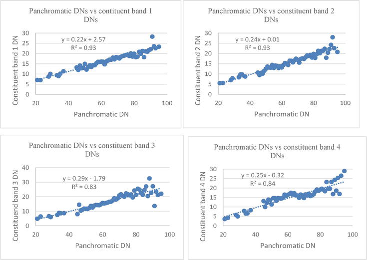
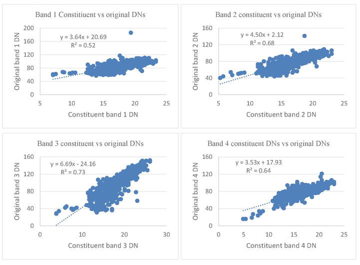
Figure 2 is a plot of the panchromatic DNs in Table 5 column 2 against their multispectral DN contributions (columns 3-6). The linear fit models and coefficients of determination are also given. Constituent contributory multispectral bands are generated by applying the above models on the panchromatic Band 8 DNs. Figure 3 shows the generated constituent multispectral DNs (Table 5 columns 3-6) versus the original multi-spectral DNs (Table 1 columns 3-6, excluding the last two records associated with the panchromatic DN 98 for the reason in Section 3.4).

Figure 2.

Panchromatic band 8 pure blocks DNs versus constituent multispectral bands DNs.

Figure 3.

Constituent multispectral DNs versus original multispectral bands DNs.

Table 6 gives the respective products of the correlation coefficients in Figures 2 and 3. From the products, it can be taken that the descending order of correctly estimating the original multispectral bands from the panchromatic band via the constituent multispectral bands is Band -2, -3, -4, -1. Consequently, Band 2 is pan-sharpened first and used as a proxy to pan-sharpen the other bands as explained below.

Band	CC1	CC2	Product
1	0.965	0.754	0.728
2	0.966	0.839	0.810
3	0.912	0.858	0.783
4	0.919	0.821	0.754

Table 6.

Products of correlation coefficients of universal panchromatic DNs versus constituent multispectral DNs (CC1) and correlation coefficients of constituent multispectral DNs versus original universal multispectral DNs (CC2).

3.6 Pan-sharpening original multispectral image

The model relating constituent Band 2 and original Band 2 is applied on the former to generate pan-sharpened band 2. The pan-sharpened Band 2 is used in pan-sharpening the other bands (Bands 1, 3, 4, 5, and 7) in the original image. At this stage, retaining the colour relationship (DNs relationship) between the original bands is critical. Tone ratio images (R_i) are computed for each original band (band_i) to the original Band 2 (band_proxy) as in Eq. (4). To generate pan-sharpened band_i, the ratio images R_i are applied on the pan-sharpened Band 2 as in Eq. (5). For instance, in the study area, the first pixel has the DN values 70, 62, 80, 62, 135, and 113 in Bands 1 through 7 (excluding Band 6) respectively. For the pixel, the ratios computed from Eq. (4) are 70:62, 80:62, 62:62, 135:62, and 113:62 for Bands 1, 3, 4, 5, and 7 respectively. The pan-sharpened Band 2 pixels of the same geographic coverage as the above original pixel have the DN values 61, 57, 61, and 64. Applying the ratio 70:62 on the pan-sharpened Band 2 pixels, Eq. (5), yields pan-sharpened-band 1 pixels with DN values 69, 64, 69, and 72, respectively. The pan-sharpened bands inherit the original colour/DN relationships of the original (non-pan-sharpened) bands through the tone ratio images. Table 7 gives the mean DNs of the original and pan-sharpened images. The means show that the original relative tone relationships are maintained.

Band	Original (1,627,527 pixels)	Pan-sharpened (6,510,108 pixels)
1	84.49 ± 12.30	84.15 ± 11.09
2	77.79 ± 14.40	77.72 ± 12.69
3	97.30 ± 25.28	96.34 ± 23.21
4	77.78 ± 11.26	79.05 ± 19.10
5	136.32 ± 32.55	136.38 ± 32.47
7	98.16 ± 27.08	97.18 ± 24.65
Tone ratio	1:0.9:1.2:0.9:1.6:1.2	1:0.9:1.1:0.9:1.6:1.2

Table 7.

DN means of original vs. pan-sharpened images.

$$R_i=\frac{ban{d}_i}{ban{d}_{proxy}}$$E4

$$Pan{B}_i=Pa{n}_{proxy}\times R_i$$E5

Where:

R_i = tone ratio image.

PanB_i = pan-sharpened band i.

Pan_proxy = pan-sharpened proxy band.

4. Results

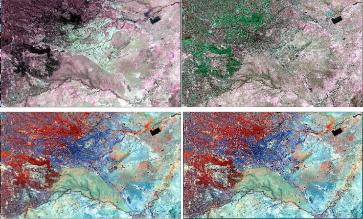
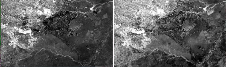
Figure 4 compares the original and pan-sharpened images. Figure 5 gives NDVI and Tasselled Cap (greenness band) images of the original image. The lighter the tone in the NDVI and greenness images, the denser the vegetation. The original image RGB = 321 captures dense vegetation as black and light vegetation as light green. This is an inconsistency. In the pan-sharpened image RGB = 321, dense and light vegetation appear as dark and light green, respectively, which is consistent with the NDVI and greenness images. The original image RGB = 457 and the pan-sharpened RGB = 457 are visually similar showing retention of colour relationship.

Figure 4.

Comparison of original and pan-sharpened multispectral images. (upper left) original bands: RGB = 321, (UR) pan-sharpened bands: RGB = 321, (LL) original bands: RGB = 457, (LR) pan-sharpened bands: RGB = 457. Dimensions in pixels; original: Y = 993, X = 1639; pan-sharpened: Y = 1986, X = 3278.

Figure 5.

NDVI image (left) and tasselled cap (greenness band) of the original image.

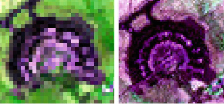
Figure 6 compares the Jomo Kenyatta International Airport hangar in the original and pan-sharpened images. In the former, the hangar appears as a blob but in the latter appears as rings as expected.

Figure 6.

Jomo Kenyatta international airport hangar – Left: Original image RGB = 342, right: Pan-sharpened image RGB = 342.

5. Discussion

The spectral range of a panchromatic band may not overlap with the spectral ranges of the encompassed bands. For the data used in this research, the panchromatic band starts at the wavelength 0.50 nm, and the collective range of the encompassed bands starts at 0.45 nm. Further, there are two spectral gaps (0.61 nm–0.62 nm, and 0.70 nm–0.75 nm) in the collective range. These gap ranges and the range 0.45 nm–0.49 nm are not accounted for in Eq. (1). This may explain the lack of perfect correlation coefficients between the panchromatic DNs and the constituent multispectral DNs (Table 6, CC1). Another source of error may be the assumption of linear combination of DNs, Eq. (1).

It is worth noting that constituent multispectral DNs versus original DNs correlation coefficients (CC2) may not be critically informative as the original DN has been split into four different DNs.

6. Recommendations

The Mix-unmix Pan-sharpener utilises a multispectral band as a proxy to pan-sharpen all the other multispectral bands after the proxy multispectral band has been pan-sharpened. The multispectral bands cover a common geographical extent. The panchromatic band of the particular sensor may not be of adequate spatial resolution depending on the end-use of the pan-sharpened image. This may call for an external finer spatial resolution panchromatic band which may not necessarily cover the entire geographical extent of the multispectral data. The problem of inadequate geographical coverage by a panchromatic band can be solved through the foregoing proxy pan-sharpening and it will be addressed in the sequel to this chapter - Mix-unmix Pan-sharpener: overcoming geographical inadequacy of panchromatic band by reverse pan-sharpening.

A mixture interval of 0.1 has been adopted for this demonstration – a comparison of different mixture intervals is necessary to establish any optimum mixture interval. The blue band has been considered as a constituent band despite it being largely not covered by the panchromatic band – does dropping it improve or worsen the results? This warrants further research. The Mix-unmix concept assumes a linear mixture of the constituent signals – there is a need for automatic determination of the mixture model. The concept needs to be assessed on hyperspectral-multispectral pan-sharpening [3, 4], optical-microwave pan-sharpening, and pan-sharpening by an external panchromatic band.

7. Conclusion

The proposed Mix-unmix Pan-sharpener can pan-sharpen any number of bands. The technique minimises colour distortion by incorporating the respective colour relationships between the original (non-pan-sharpened) bands and the proxy pan-sharpening band through tone ratio images, in the generation of respective pan-sharpened bands.

Acknowledgments

The data is downloaded from [21].