Disasters and Housing Infrastructure: Evidence from the 2010 Chilean Earthquake

Abstract

In 2010, a severe earthquake occurred in Chile that brought high-impact destruction effects in the affected areas. It has studied the damage to homes, the determiners of the cost of reconstruction, and how households finance reconstruction using the Casen post-earthquake 2010 panel survey. A probit and an OLS model were used. The results show that houses closest to the epicentre were the most affected, where damage increased when roofs and walls were in worse condition or with more vulnerable materials. The reconstruction costs are related to the degree of destruction, the distance to the epicentre, the condition of the walls before the event and the house’s value. Provinces with more bank branches are associated with a lower cost. Bank credit is more likely to be used to rebuild in urban areas, when the head of the household has more years of education and when the repair cost is higher. Own savings will be used when there is no insurance, the higher the income of the head of household and the lower repair costs. Finally, subsidies will be an option when there is no insurance, the repair cost is higher, and for lower income, age, and education.

1. Introduction

Throughout human history, we have lived with great-scale natural phenomena that have generated all kinds of losses, altering both the dynamics of communities and the economic activities associated with the affected areas. The United Nations has carried out projects that have allowed the increase of attention toward the diverse threats with which man has to live, amongst the most highlighted is the International Natural Disaster Reduction Decade [1]. In the same manner, a series of development policies at an international level have focused on the protection of the vulnerable related to avoidable losses, leaving natural disasters as an exceptional fact that is not part of the development theory [2]. However, social media and technology have taken a fundamental role in our lives, and this has increased the investigation in the natural science areas with the goal of improving the capacity to anticipate these disasters, face them, and mitigate their consequences.

Chile, located within the Pacific Ring of Fire, finds itself in constant exposure to earthquakes across its territory [3, 4]. These occurrences bring not only damage to homes and infrastructure but also high economic and social costs linked with reconstruction efforts [5, 6, 7]. This vulnerability was demonstrated when a seismic event on February 27th, 2010, struck. It registered a magnitude of 8.8, making it the sixth most powerful earthquake globally, and the second-largest earthquake ever recorded in Chilean history [8]. The earthquake’s epicenter was offshore, near the Maule Region, with a focal depth extending to approximately 35 kilometers beneath the Earth’s surface. This earthquake significantly affected six out of the country’s 15 regions, encompassing an expanse of 700 kilometers, where 80% of the population resides [9]. The losses incurred by this event were estimated at 30 billion dollars, equivalent to 18% of the GDP [10]. Figure 1 illustrates the extent of the affected zone by the earthquake and the regions involved.

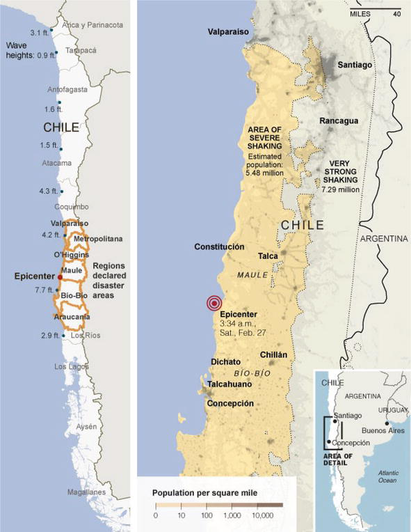
Figure 1.

Area affected by the earthquake in Chile, 2010. Source: [11]; United States geological survey (USGS) for epicentral location data.

In the aftermath, as Chile confronted the intricate interplay of physical destruction and social upheaval, the event stood as a lasting testament to the importance of fortifying preparedness, response, and mitigation efforts. It underscored the necessity of adopting a multidimensional approach that considers both the tangible losses of infrastructure and the intangible yet equally significant fabric of communities and societies. Amid an era marked by the proliferation of technology and the interconnectivity fostered by social media, the lessons drawn from this earthquake have spurred the exploration of innovative scientific avenues to enhance prediction, response strategies, and ultimately, the reduction of the toll exacted by natural disasters.

This earthquake is particularly interesting to be studied due to its magnitude, coverage, and quantity of homes affected. For this purpose, there is panel data with information at the home level that allows us to explore the destructive power of the disaster and its socioeconomic effects. This chapter explores the following questions: How does the distance of the earthquake’s epicenter affect the probability of home damage, considering the state of the construction before the event? What are the primary factors influencing the cost of home reconstruction? Additionally, how do homeowners secure financing for their home repairs or reconstruction? Does the access to banking institutions affect the cost and capacity of the reconstruction? In Section 2, The economic impact of natural disasters a literature revision is conducted, in Section three Methodology, the used data and estimated models are described, in Section 4, Results the empirical results are presented in conjunction with the robust tests, and finally, in Section 5, Conclusion the main conclusion are presented.

2. The economic impact of natural disasters

A natural disaster is a catastrophic event caused by natural forces or processes that result in significant damage to the infrastructure of settlement, infrastructure damage, the loss of life, economic costs, and socio-environmental disruption in general. These events are out of human control and can have devastating consequences for the areas and affected populations [12]. Some examples of natural disasters include hurricanes, earthquakes, floods, forest fires, tsunamis, volcanic eruptions, and tornados. Although natural disasters mainly originate from natural factors, human activity might influence the gravity and impact. These are known as human factors or man-induced factors, which we can identify [13]:

1. Terrain and house development usage: Human settlements and infrastructure located in vulnerable areas can increase the risk and amplify the impact of natural disasters. For example, the construction in flood propensity planes or in unstable slopes can produce greater damages through floods or landslides.

2. Land degradation and deforestation: The logging for agriculture or housing development reduces the natural barriers against disasters. Trees play a crucial role in the prevention of land erosion, water flow regulation, and the mitigation of the impact of events, such as floods and landslides.

3. Climate change: Man-made climate change is altering the climate patterns and increasing the frequency and intensity of some natural disasters. The global temperature increase can contribute to the creation of hurricanes, heat waves, droughts, and severe storms.

4. Deficient housing infrastructure and planning: The inadequate housing planning, the inadequate zoning, and the weak infrastructure can exacerbate the impact of disasters. For example, inadequate drain systems can produce an increase in floods, and poorly constructed buildings are more susceptible to crumbling during earthquakes.

5. Overcrowding and population growth: The rapid population growth, particularly in areas prone to threats, can put more people at risk during a natural disaster. Overcrowding and inadequate preparation for emergencies can obstruct the efforts of evacuation and increase the number of victims.

6. Early alert and lack of preparation: Insufficient preparation for disaster, including the absence of early alert systems, can make the evacuation and opportune response more difficult. Education and awareness about natural dangers, as well as effective emergency planning, are crucial to mitigate the impact of disasters.

With it, natural disasters have been studied from different perspectives, including damage evaluation of infrastructure, risk mitigation, emergency preparation, preventive measures, logistic, social, work, sanitary, environmental, and economic effects amongst others [12].

Amongst the related studies of natural disasters, we find a line that estimates the social or economic costs that a seismic event generates in the zones, where it impacts. This line of study, the World Bank [14, 15] shows that the economic and social cost has increased in the last years due to growth in population. It also shows that the loss of life and the destruction of infrastructure in natural disasters delay every type of program that has as objective the overcoming of poverty given that it generates deviation of resources for recovery and reconstruction.

On the other hand, Sen [16] establishes that the associated costs of natural disasters are determined mainly by economic and social factors above the magnitude of the process. As an example, it points out the earthquakes occurred in Haiti and Chile in the year 2010, in which the first caused the death of 200.000 and 250.000 people and damages to the economic infrastructure of the country in more than 100% of the PIB of the country [17], while the second registered a greater intensity but caused less than 500 deaths and fewer damage to Haitians in relation to the size of its economy [18]. In this sense, it can be established that natural disasters cause great economic losses all over the world; however, the damage caused has a direct relation with the country’s income [19]. Even though the economic losses are greater in developed countries, they are less in proportion to their PIB in comparison to developing countries [20].

The damages caused by natural disasters can be classified between direct damages and indirect damages [2]. The direct damages correspond to the damages of the fixed assets, capital, raw materials, extractable natural resources, mortality, and mobility as a direct consequence of the disaster. The indirect damages are related to the production of estates and services that will not be able to function after the disaster, additional costs that are incurred due to the necessity of producing or distributing alternative assets, and the loss of resulting incomes due to lack of provision of assets and services or the destruction of the production. Additionally, the secondary effects correspond to those that have incidence in the global economic performance, and which measurement is performed through the macroeconomic variables such as the PIB, the commercial scale, the payment balance, the debt level, international reserves, and investment [21], where the sensitivity of a country in the face of the impact of natural disasters can increase according to its level of economic development. Kahn [22] concludes that in the richest countries less deaths are generated in the face of natural disasters of equal severity.

For its part, there is a series of studies oriented at quantifying the impact of a natural disaster, the financial risk associated, and the recovery time. Within this economic study, we find a strong emphasis on the analysis of the relationship between the economic situation of the government, the foreigner relations, and the level of maturity of the financial industry, especially in the insurance market and the risk transfer [23, 24, 25, 26, 27]. In relation to the recovery and the reconstruction at the microeconomic level, Noy [28] establishes that the financial flows play an important role in the recovery of disaster; therefore, the conditions of the financial market are another factor to consider to evaluate the consequences of natural disasters. It also points out that the bigger the domestic credit the costs of the disaster are reduced [17, 29, 30, 31].

Benson and Clay [14] study the economic impact of natural disasters considering government spending and the redistribution of resources to finance the initiative of the government. They identify that the disasters generate additional costs or partial financial resources reassignment that are destined for reconstruction, rehabilitation of public assets, and relay support for the victims. For the insurance and private capital support to be effective in the reduction of the impact of natural disasters, it is necessary to perform planning and assignments of funds that allow it to fulfill the consequences in an anticipated manner, as well as the mitigation and preparation of support. They conclude that the reassignment of funds after a disaster must be carried out through a formal process, designed after a careful strategic revision, and that it is necessary to increase the financial mechanisms that manage to correctly perform the risk transfers between different types of disasters and the impact mitigation.

In the same manner, Ghesquiere & Mahul [32] perform a financial analysis of both public and private with the objective of supporting the development of financial protection in the face of natural disasters related to different risk levels. It also identifies that for developing countries is of great importance to develop financial strategies given their greater vulnerability, as opposed to developed economies that possess a greater and prolonged usage of resources dedicated to reducing vulnerability, such as buildings with better structure or legislative systems that are more demanding in terms of usage of land and construction. It proposes that the recovery strategy must be tackled with public resources, as well as with private resources in relation to the frequency and severity of the risks so as to create a strategy of financial instruments according to the severity and frequency of each type of disaster. The proposal is summarized in Table 1.

Frequency	Severity	Risk	Financial instrument
Low	Major	High-risk layer	Risk insurance for disasters
Mid	Mid	Mid risk layer	Contingency credit
High	Minor	Low-risk layer	Contingency budget and annual budget assignment

Table 1.

Financial strategy according to risk and severity.

Source: Elaborated based on Ghesquiere & Mahul [32].

The financial protection strategies address the symptoms and not the cause of catastrophes; therefore, a good strategy may help diminish the financial impact that a calamity can generate. However, it is important to point out that in a global strategy of catastrophe risk management financial protection is only one component. These sources of finance are separated into those delivered before and after the disaster. The tools that come after are sources that do not require planning such as the realignment of the budget, internal credit, external credit tax increase, and the help of donors. The financial tools of risk ex ante require anticipated planning and include disaster funds or reserves, budgetary contingency, and mechanisms of risk transference [32].

It is important to count on evaluation systems of natural disaster impacts, evaluate the fiscal sustainability, and vulnerability of the governments and have an optimal financial structure for the retention of risks and the transfer taking into account the contingency credits, reserves funds, insurance, and catastrophe bonuses [25].

Finally, there are studies that relate socioeconomic characteristics with the way natural disasters impact, and in these, it is indicated that when there is clear information about the risk zones, the homes located in the riskier zones are more expensive and are, therefore, in less demand, which should reduce the damage by natural disaster in the future [33].

3. Methodology

To perform the study different sources were used. First, the data panel house survey CASEN post-earthquake 2010 was used, of which the population sample reaches 75.986 people and 21.899 homes samples, which contain socioeconomic information at the home level. Second, the distance of the earthquake’s epicenter distance in relation to the communal capital was used where the home was located, information that was constructed for the elaboration of the present study taking the distance in kilometers between the provincial capital and the epicenter. Finally, the number of banking branches that existed in each province in the year 2010 was used according to the information delivered by the superintendence of banking and financial institutions (SBIF).

In our analysis, we employed a controlled regression analysis approach to assess the relationships between predictor variables and the outcome variable. To ensure accurate and meaningful results, control variables were incorporated into the regression models. The inclusion of control variables is a common practice in statistical analysis to account for potential confounding effects and enhance the precision of our findings.

For the purpose of clarity and interpretation, we denoted the inclusion of control variables using the notation “YES” in the table, and this means that the regression models were constructed with the consideration of additional factors that could influence the outcome variable. In addition, we consider R-squared metrics that indicate how much of the variation of a dependent variable is explained by the independent variables in our recession model. In other cases, we used the term “Pseudo R-squared” to refer to the coefficient of determination (R-squared) when the explained variable is categorical and the coefficient of determination cannot be applied. This approach is similar to R-squares, and they have a similar scale (from 0 to 1) and higher values indicate a better model.

Incorporating control variables aims to ensure that the analysis captures a comprehensive view of the relationships under investigation. This approach allowed us to mitigate potential bias and produce results that reflect the genuine influence of the predictor variables on the outcome variable.

The investigation questions are addressed from three thematic: home damage, reparation costs or home reconstruction, and financial sources.

3.1 Home damage

To study the relation between the earthquake epicenter distance and the home damage, a nonlinear probability model of binary selection probit is used (Eq. 1), where the explained variable corresponds to the damage of the home that can have values 1 or 0 (where 1 indicates that the homes were damaged and 0 that there was no damage as consequence of earthquake or tsunami). The explanatory variables considered are the distance from the home to the epicenter of the earthquake (${\mathit{Dis}}_i$) and a categorical variable of control ($X_i$) that indicates the type of holding of the home, the material of the construction of the home, and its conservation status. Thus, model is as follows:

$$\mathit{PR}\left({\mathit{\text{Damage}}}_i=1\right)=F\left(\alpha +\beta {\mathit{Dis}}_i+\gamma X_i\right)$$E1

Where PR corresponds to the probability, F is the function of the accumulated normal standard of distribution, and the subindex $i$ corresponds to the home. The parameters $\alpha$, $\beta ,$ and $\gamma$ were estimated by the maximum likelihood estimation. The results can be interpreted in probability terms so that the sign of parameter estimates indicates the direction in which the probability moves each time the explanatory variable increases. Subsequently, the interaction between $\mathit{Dis}$ and $X$ is included to evaluate if the earthquake has affected the homes in poor conditions in spite of the distance of these from the epicenter.

3.2 Repair cost

In relation to the main determiners of the costs of reconstruction or repairs of a home, we estimate an ordinary least squares (OLS) regression models (Eq. 2), where the dependent variable is the costs of repair or reconstruction of the home (Cost), and the explanatory variables considered are: the type of property of the home, the number of banks, the damage degree of the home, the rent value of the home, the distance of the epicenter, and the state of conservation of the walls, floors, and roofs, leaving the model to estimate as follows:

$${\mathit{\text{Cost}}}_i=\alpha +\beta {\mathit{\text{Prop}}}_i+\vartheta {\mathit{Ban}}_i+\eta {\mathit{\text{Damage}}}_i+\rho {\mathit{Ren}}_i+\gamma {\mathit{Dis}}_i+\delta X_i+\epsilon$$E2

Where ${\mathit{\text{Cost}}}_i$ represents the estimated cost of the homes repars in millions of pesos, the variable ${\mathit{Ban}}_i$ represents the number of banks that are in the province, and the degree of damage of the home ${\mathit{\text{Damage}}}_i$ is the variable that may take values 0,1,2, and 3 and represents a home without damage, with minor damages, major damages, or destruction due to the earthquake, respectively; the value of rent of the home ${\mathit{Ren}}_i$ indicates how much rent is paid by the home or how much it would cost if it were to be paid, ${\mathit{Dis}}_i$ is the distance of the epicenter and $X_i$ represents the state of conservation of the walls, floors, and roof. The parameters $\alpha$, $\beta$, $\vartheta$, $\eta$, $\rho ,\gamma$, $\mathit{\text{and}}\delta$ were estimated by the ordinary least squares method that allows us to find the parameters that minimize the sum of the squared residuals in a linear regression model.

3.3 Financial sources

To understand how homes finance their reconstruction or repair a probit binary nonlinear selection of probability is used (Eq. 3), where the explained variable corresponds to the options of finance be it from banks, savings, or subsidies (${\mathit{Fin}}_i$), and the considered explanatory variables are the home’s income, age, education level, area, cost of reconstruction, insurance, number of banks, and distance of the epicenter of the home i.

$$\mathit{PR}\left({\mathit{Fin}}_i\right)=F\left(\alpha +\beta {\mathit{Inc}}_i+\vartheta {\mathit{Age}}_i+\eta {\mathit{Edu}}_i+\rho {\mathit{Rur}}_i+\gamma {\mathit{\text{Cost}}}_i+\delta {\mathit{\text{Insu}}}_i+\mu {\mathit{Ban}}_i+\xi {\mathit{Dis}}_i\right)$$E3

Where the financial options can be from banks, savings, or subsidies and can take the values 1 or 0 (where 1 indicates that the home utilizes that option, and 0 that it does not). The considered explanatory variables are the home’s income $\left({\mathit{Inc}}_i\right),\mathit{\text{the}}\mathit{age}\left({\mathit{Age}}_i\right),$ education level $\left({\mathit{Edu}}_i\right)$, rural zone (${\mathit{Rur}}_i$ variable that indicates if the home belongs to a rural zone or not), ${\mathit{\text{Cost}}}_i$ represents the cost of the reconstruction or repair of the home, insurance (${\mathit{\text{Insu}}}_i$ variable that indicates if the home has insurance or not), the number of banks (${\mathit{Ban}}_i)$, and distance from the epicenter (${\mathit{Dis}}_i$). The parameters $\alpha$, $\beta$, $\vartheta$, $\eta$, $\rho ,\gamma$, $\delta$, $\mu \mathit{\text{and}}\xi$ were estimated by the maximum likelihood estimation, and the results can be interpreted in probability terms so that the sign of parameter estimates indicates the direction in which the probability moves each time the explanatory variable increases.

Finally, to verify the consistency of the statistical models, the statistical t was calculated, and the significance level of each variable was determined, as well as the coefficient of determination of each model.

4. Results

The preliminary results in relation to the number of affected homes, and the type of damage received show that 33.22% of the country’s homes had some kind of damage after the earthquake and also after the tsunami. Specifically, 21.91% of homes showed minor damages, 8.06% major damages, and 3.24% were destroyed due to the earthquake or later due to the tsunami. These results are observed in Table 2.

	All provinces		Affected provinces
	Number of homes	Percentage	Number of homes	Percentage
Destroyed by earthquake	643	2.94	643	3.69
Destroyed by tsunami	66	0.30	66	0.38
Major damage	1.766	8.06	1.732	9.93
Minor damage	4.799	21.91	4.715	27.04
Not affected	14.625	66.78	10.280	58.96
Total	21.899	100	17,436	100

Table 2.

Number of homes affected according to the type of damage.

Source: Own elaboration.

In relation to the construction material of the homes under the study, the majority of homes were built from bricks (43.39%), followed by wood partition lined on both sides (36.42%), and in third place a small percentage of the constructed homes were adobe, wooden partition without linings and reinforced concrete (around 7% each one). In general, 20% of the homes showed some kind of damage prior to the seismic event, that is to say, they had poor conditions in some parts of the construction such as walls, roof, or floor. These results are observed in Table 3.

Construction material	Destroyed homes	Destroyed homes
	% of the total homes	% of the construction material
Reinforced concrete	6.56	1.1
Brick	43.39	1.46
Wood partition lined (both sides)	36.42	1.52
Adobe	6.72	23.99
Wood partition unlined	6.82	2.74
Mud houses	0.36	17.33
Waste/recycled material	0.05	13.51
Others	0.02	0
Total	100

Table 3.

Number of homes destroyed according to the construction material.

Source: Own elaboration.

In relation to the destruction of the homes due to the earthquakes, we can point out that de adobe houses are the pens that show a higher rate of destruction (23.99% of adobe houses were destroyed), followed by mud houses (17.33% of them) and those built from waste material or recycled material (13.51% of them). We can conclude that the destruction of the homes has a direct relation with its construction material. This can be observed in Table 3.

4.1 Estimated models

In this section, the results of the estimated models are shown. It is important to note that the significance of the model attributes is evaluated according to the p-values with the standard scale where [34]:

1. p < 0.01 is considered highly statistically significant. It suggests that there is strong evidence to reject the null hypothesis, indicating a substantial effect or relationship in your analysis. This case is represented by three asterisks (***).

2. p < 0.05 indicates that there is statistically significant evidence to reject the null hypothesis, implying a meaningful effect or relationship. This case is represented by two asterisks (**).

3. p < 0.1 indicates that there is weak evidence against the null hypothesis, and the effect or relationship may be borderline significant. This case is represented by one asterisk (*).

The results of the first estimate shown in the methodology are presented in Table 4. These show that the type of property occupancy has a correlation with the home damage. In particular, owning a house or renting relates to a lesser probability of damage or destruction, with a significance of at least 5% while an irregular home occupancy is related with a higher probability of damage. The negative sign on the probability of housing damage (e.g., −0.0497 for “owned”) indicates that there is a 4.97% lower probability that an owned home will be damaged.

	Damage	Major damage	Destruction
Owned	−0.0497***	−0.0289***	−0.0099***
Rented	−0.0279*	−0.0162*	−0.0048*
Irregular	0.0492	0.0542*	0.0038
Distance	−0.1011***	−0.0327***	−0.0101***
Poor wall condition	0.0801***	0.0676***	0.0189***
Poor floor condition	0.0276*	0.0117	−0.0019
Poor roof condition	0.1347***	0.0420***	0.0044
Fixed construction material effect	YES	YES	YES
Fixed region effect	YES	YES	YES
Observations	17,435	17,435	17,419
Pseudo R-squared	0.128	0.180	0.282

Table 4.

Probability of home damage.

***p < 0.01, **p < 0.05, *p < 0.1. Results elaborated by authors based on post-earthquake survey.

Second, we find a relationship between the distance from the epicenter and the damage level or destruction with a significance of 1% evidencing that the further the distance lesser the damage. Specifically, it means that as the distance to the earthquake epicenter increases by 200 kilometers, the probability of experiencing housing damage decreases by 10.11% (highly statistically significant). Similarly, the probability of experiencing housing major damage decreases by 3.27% and destruction by 1.01%. This means that homes farther away from the epicenter are substantially less likely to suffer damage, major damage, or destruction during an earthquake. However, this is an intuitive result, given that the earthquake’s epicenter intensity is greater and lessens as we move away from this spot.

Lastly, in relation to the poor quality of walls, the variable is highly significant to 1%, and the results show that it relates with a greater probability of damage or destruction, while the poor quality of floor or roof only correlates with damages and not destruction.

In the second estimate, we incorporate the variable between distance and the state of the conservation of the homes to evaluate if the earthquake has actually affected the homes in poor conditions, in spite of the distance from the epicenter. First, we evidence the correlation between the distance from the epicenter and the damage or destruction of the homes. Second, the type of occupancy of the property also shows a correlation with the damage of the home. In particular, an owned or rented home is related to a lesser probability of damage or destruction, while an irregular occupancy of a home is related to a higher probability of major damage. Third, it can be said that the poor conditions of the walls and the roof are related to a higher probability of damage and destruction, while the poor quality of the floor only correlates to damage. Lastly, the included interaction indicates that the homes in poor conditions have less probability of major damage if they are located farther from the epicenter.

Therefore, for all types of damage (damage, major damage, and destruction), variables that are highly statistically significant are: 1) Distance, where negative coefficients (−0.0993, −0.0305, −0.0097) indicate that increasing distance from the earthquake epicenter significantly reduces the probability of home damage, 2) Owned: Owning a house increase the probability of experiencing damage, major damage, and destruction decreases significantly were highly statistically significant (***), for all three types of damage, the negative coefficients (−0.0499, −0.0292, and − 0.0100) suggest that probability of experiencing damage, major damage, and destruction decreases significantly, 3) Poor wall condition, where positive coefficients (0.0950, 0.0838, 0.0235) indicate that poor wall condition significantly increases the probability of all types of damage, and 4) Poor roof condition, where positive coefficients (0.1501, 0.0568, 0.0073) indicate that poor roof condition significantly increases the probability of all types of damage. For all types of damage, the variable “poor floor condition” is statistically significant and the variable “irregular” is marginally statistically significant for “destruction” (p < 0.1). It has a positive coefficient (0.0564) suggesting that irregular homes may have a slightly higher probability of experiencing destruction, but this result is less robust than the highly significant variables. In summary, distance, poor wall condition, and poor roof condition are highly statistically significant predictors of all types of damage, with distance having a negative effect, and poor wall/roof condition having a positive effect. Poor floor condition is statistically significant but at a lower level (p < 0.05) for all types of damage, with a positive effect. Irregular construction type is marginally significant (p < 0.1) for “destruction” only, with a positive effect. The interaction term “distance*poor quality” is not statistically significant for any type of damage. The results obtained are similar to the previous model and are presented in Table 5.

	Damage	Major damage	Destruction
Owned	−0.0499***	−0.0292***	−0.0100***
Rented	−0.0280*	−0.0163*	−0.0048*
Irregular	0.0509	0.0564**	0.0042
Distance	−0.0993***	−0.0305***	−0.0097***
Poor wall condition	0.0950***	0.0838***	0.0235***
Poor floor condition	0.0416**	0.0238**	0.0001
Poor roof condition	0.1501***	0.0568***	0.0073*
Distance*poor quality	−0.0051	−0.0046**	−0.0010
Fixed construction material effect	YES	YES	YES
Fixed region effect	YES	YES	YES
Observations	17,435	17,435	17,419
Pseudo R-squared	0.128	0.180	0.282

Table 5.

Probability of home damage.

***p < 0.01, **p < 0.05, *p < 0.1. Results elaborated by authors based on post-earthquake survey.

To respond to the second investigation question that has relation to the main determinants of the reconstruction cost, two estimates were conducted, and the results obtained are presented in Table 6. We can see that there is a correlation between the degree of damage and the cost of repair or reconstruction of the home, and an intuitive result given that the repair cost of a house with small damages should be less than the cost of the complete reconstruction. In addition, we observe a correlation between the rent and cost variables, in particular, the higher the rent value of the house, the greater the cost of its repair.

	(1); Cost	(2); Cost	(1); Cost	(2); Cost
N° banks	−0.0003***	−0.0003**	−0.0002*	−0.0003**
Degree of damage	1.2466***		1.1627***
Rent	0.0030***	0.0021***	0.0029***	0.0025***
Distance from the epicenter		−0.1126***		−0.0501
Quality of the wall		0.1852**		0.1847**
Quality of the floor		0.0392		0.0581
Quality of the roof		−0.0053		0.0345
Constant	1.8349***	2.5043***	1.7721***	2.0628***
Fixed construction material effect	NO	NO	YES	YES
Fixed region effect	NO	NO	YES	YES
Observations	3309	3275	3275	3275
R-squared adjusted	0.3280	0.1018	0.3450	0.1173

Table 6.

Estimated coefficient of the cost of repair/reconstruction.

***p < 0.01, **p < 0.05, *p < 0.1. Results elaborated by authors based on post-earthquake survey.

Therefore, in this analysis of “cost,” the number of banks consistently demonstrated a negative effect on cost, with coefficients ranging from −0.0003 to −0.0002, suggesting that an increase in the number of banks is associated with lower costs of repair of the home. However, as the degree of damage increased across various model setups, “cost” also increased significantly, with coefficients ranging from 1.1627 to 1.2466, indicating that more severe damage is consistently linked to higher costs. Higher rental costs were positively associated with “cost” in different model specifications, with coefficients ranging from 0.0021 to 0.0030, suggesting that areas with higher rental prices tend to have higher costs. Greater distance from the earthquake epicenter was found to significantly reduce “cost”in certain model configurations, with a coefficient of −0.1126, while the quality of walls was positively associated with “cost” in various model setups, with coefficients ranging from 0.1847 to 0.1852 (which is to be expected given that the closer it is to the epicenter it generates more damage and vice versa.). Additionally, better roof quality was associated with higher “cost” in (4) model specifications, with a coefficient of 0.0345. However, the quality of the floor did not show a statistically significant effect on “cost” in certain model specifications but was positively related to “cost” in others, with coefficients ranging from 0.0392 to 0.0581. These findings provide valuable insights into the determinants of “cost” across different configurations of control variables.

This is congruent with our previous results that showed that in the epicenter the damage is greater, and therefore the cost of the repair should be greater. We also noticed that the walls in poor condition before the disaster are related to a more expensive repair. Just like in the previous model, a positive correlation is observed between the rent and cost variables, and we can observe that a greater number of banks is related to a lesser cost of repairs. Finally, the field material and region effects were included, and the results obtained are similar, only the variable of significance is lost that now captures the controls of the region.

When we consider the costs of repair or reconstruction obtained from technical agencies or construction specialists, the results obtained differ slightly and are shown in Table 7. We see a correlation between the degree of damage and the cost of repair of the homes; however, this correlation is slightly less in comparison with the previously obtained by the homeowner. In the same way, there is a positive correlation between the rent and cost variables, and we observe that a greater number of banks is related to a lower cost. The second estimate shows different results, given that it only evidences a relation between the distance from the epicenter and the cost of repair of the home, showing that at a greater distance, the cost diminishes. Finally, the fixed construction material effects and the fixed region effects are similar, there is only a loss of significance with the variables of distance that now are captured by the control of the region and the number of banks.

	(1); Cost	(2); Cost	(1); Cost	(2); Cost
N° banks	−0.0006**	−0.0004	−0.0004	−0.0003
Degree of damage	1.1673***		1.1405***
Rent	0.0018**	0.0008	0.0019***	0.0012
Distance of the epicenter		−0.1363***		−0.0625
Quality of the wall		0.1836		0.1434
Quality of the floor		0.0861		0.1435
Quality of the roof		−0.1543		−0.1313
Constant	2.7372***	3.5500***	2.6171***	3.0830***
Fixed construction material effect	NO	NO	YES	YES
Fixed region effect	NO	NO	YES	YES
Observations	755	755	755	755
R-squared adjusted	0.3628	0.1287	0.3650	0.1387

Table 7.

Estimated coefficient of the cost of repair/reconstruction (technical agencies).

***p < 0.01, **p < 0.05, *p < 0.1. Results elaborated by authors based on post-earthquake survey.

In relation to how homes finance their repair or reconstruction and considering three different financial sources, Table 8 shows the results obtained in the estimates. They indicate that homes that have earthquake insurance have a lesser probability of financing their repair or reconstruction with their own savings or subsidies. In relation to the income level of homes, it can be observed that the higher incomes are related with a greater probability of home repair financed by savings, and it is correlated with less probability of obtaining subsidies. In the same way, we noticed that older homeowners have more probability of financing the repair with savings and less subsidies. The education level of the homeowners also affects the type of finance given to them, given that higher level of education is related to higher bank financing and savings and with less subsidies. The houses located in rural zones have less probability of obtaining banking finance, as well as in zones, where there is a bigger number of banks. Lastly, the variable, the estimated cost of repair is correlated with the three sources of finance: a greater cost is related to higher probability of banking finance and subsidies, and at the same time with less financing of saving.

	Bank	Savings	Subsidies
Insurance	0.0221	−0.0505*	−0.0794***
Income	−0.0034	0.0571***	−0.0662***
Age	0.0005	0.0010*	−0.0018***
Education	0.0039***	0.0041*	−0.0115***
Rural Zone	−0.0556***	0.0080	0.0142
N° banks	−0.0001**	−0.0001**	0.0000
Cost	0.0229***	−0.0985***	0.0892***
Fixed construction material effect	YES	YES	YES
Fixed region effect	YES	YES	YES
Observations	3869	3869	3869
Pseudo R-squared	0.0463	0.0746	0.117

Table 8.

Probability related to financial sources of reconstruction.

***p < 0.01, **p < 0.05,*p < 0.1. Results elaborated by authors based on post-earthquake survey.

5. Conclusions

Earthquakes generate damages and losses of infrastructure, and the reason that motivated the study of variables that affect the damage of a home, the main determiners of costs of the reconstruction, and how homes finance the reconstruction. The study is focused on the Chilean earthquake of 2010 and microdata was utilized from home surveys performed for three months after the disaster.

In relation to the destruction of homes, the results show that houses built from adobe are the ones that showed a higher rate of destruction, followed by mud-built houses, quincha, and pirca. In relation to the connection between the distance from the epicenter of the earthquake and the damage of a home, the results show that the houses located closer to the epicenter were, on average, more affected by the earthquake. This effect is stronger in houses that had already deteriorated before the disaster, mainly in those that had walls in poor condition.

The second group of results shows that the costs of reconstructions associated with the earthquake are related to the degree of destruction of the house, the distance from the epicenter, the condition of the walls before the event, and the value of the house. The number of banking branches in the province is related to a lower cost of repair, being related to the results obtained by Atienza and Aroca [35], where a discussion is held on what relation there is between the spatial concentration and efficiency, which allows the diminishment of the commercial cost. Just like Noy [28] who observed that the internal credit reduces the cost of disaster in growth terms of the lost product, this work puts in evidence that the greatest competition of internal credit helps reduce the cost in terms of price.

These findings may have policy implications for disaster preparedness and recovery in Chile. Areas with a higher concentration of banks might have better access to financial resources or services that could aid in post-earthquake recovery efforts. Policymakers and disaster response agencies could consider leveraging this information to prioritize resource allocation and support in regions with less financial support. While the negative relationship between the number of banks and earthquake-related costs is noteworthy, further investigation may be needed to understand the underlying mechanisms. Exploring why regions with more banks tend to have lower costs could provide valuable insights for disaster planning, as well as explore why access to banking services, capital, and financial resources can significantly impact a community’s ability to withstand and recover from natural disasters. By investigating the presence and role of banks or, in general, financial support in these areas, could be a contribution to the development of more effective disaster risk reduction and recovery policies.

Finally, it is characterized by how homes finance the reconstruction of their houses. Specifically, the study found that homes with higher incomes have more possibilities of financing the reconstruction with savings, while the homes of lower incomes are more prone to finance the reconstruction with subsidies from the government or other institutions. The families that live in rural zones have less possibilities of financing the reconstruction with banking entities. The bigger the cost of the reconstruction, the homes are less prone to finance with savings, and the probability of finance by banking loan or subsidies is increased. With all this, the human factors highlight the importance of comprehending and tackling the role of social and economic activities in relation to natural disasters. Once we recognize and tackle these factors, societies can take proactive measures to reduce the vulnerability and increase the resilience in the face of natural disasters.

In the course of this study, we have employed the epicentral distance as a key parameter in our analysis. However, in light of the extensive rupture areas observed in certain seismic events, it is prudent to consider alternative distance metrics to enhance the precision and scope of our analysis. Utilization of metrics, such as the Joyner & Boore distance, which accounts for the closest distance to the surface projection of the rupture, or even measuring the closest distance to the rupture itself, can be pivotal in capturing a more nuanced understanding of seismic events characterized by significant rupture areas. The potential benefits of adopting these alternative distance metrics are evident as they may provide improved insights and more accurate predictions. It is important to acknowledge that the current study has been conducted under the constraints of available data, and thus, our exploration has centered around the epicentral distance. Despite the acknowledged potential for improved results through the use of alternative metrics, the present study remains anchored within the available data landscape.

As a suggestion for future research, we recommend the integration of these alternative distance metrics, such as the Joyner & Boore distance or the closest distance to the rupture, into the modeling framework. This extension could yield valuable insights, expanding the depth of analysis, and broadening the applicability of our findings. We believe that this line of research could lead to a more complete and accurate understanding of seismic events, especially those that generate large areas of rupture. We hope that future researchers can explore these metrics and assess their impact on seismic event analyses, which will ultimately improve our understanding of and ability to react to catastrophic events.

References

- 1.
Lavell A, Latina A. Viviendo en riesgo. In: Comunidades Vulnerables y Prevención de Desastres en América Latina. Compilador. Colombia: La Red, FLACSO, DEPREDENAC; 1994 - 2.
Pelling M, Özerdem A, Barakat S. The macro-economic impact of disasters. Progress in Development Studies. 2002; 2 (4):283-305 - 3.
Cisternas M, Atwater F, Torrejón F, Sawai Y, Machuca G, Lagos M, et al. Predecessors of the giant 1960 Chile earthquake. Nature. 2005; 437 :404-407 - 4.
Lagos M. Tsunamis de origen cercano a las costas de Chile. Revista de Geografía Norte Grande. 2000; 27 :93-102 - 5.
Hube MA, et al. Repaired Reinforced Concrete Wall Buildings in Chile after 2010 Maule Earthquake. In: 11th US National Conference on Earthquake Engineering. 2018 - 6.
Jünemann R, De La Llera JC, Hube MA, et al. A statistical analysis of reinforced concrete wall buildings damaged during the 2010, Chile earthquake. Engineering Structures. 2015; 82 :168-185 - 7.
Noji EK. The public health consequences of disasters. Prehospital and disaster medicine. 2000; 15 (4):21-31 - 8.
USGS - 20 Largest Earthquakes in the World, online. Available from: https://www.usgs.gov/programs/earthquake-hazards/science/20-largest-earthquakes-world-1900 - 9.
CEPAL. Terremoto en Chile Una primera mirada al 10 de marzo de 2010, Copyright © Naciones Unidas, marzo de 2010. https://www.cepal.org/noticias/paginas/4/35494/2010-193-terremoto-ev1.pdf - 10.
Comerio MC. Housing Recovery in Chile: A Qualitative Mid-Program Review. Berkeley, CA: Pacific Earthquake Engineering Research Center Headquarters at the University of California; 2013 - 11.
The New York Time, 2010. Maps of the Chile Earthquake [online]. [image]. 2010. [Accessed 3 March 2019]. Available from: https://archive.nytimes.com/www.nytimes.com/interactive/2010/02/27/world/americas/0227-chile-quake-map.html?hp - 12.
David A. Natural disasters. 1st ed (July 3, 2017). New York, NY, USA: Routledge; 2017. ISBN-10: 1138424374 - 13.
Verstappen HT. Natural and human factors in environmental disasters. Geographia Polonica. 2003; 76 (2):1-40 - 14.
Benson C, Clay E. Understanding the Economic and Financial Impacts of Natural Disasters. Washington, D. C.: The World Bank; 2004 - 15.
Hallegatte S. The indirect cost of natural disasters and an economic definition of macroeconomic resilience. World Bank Policy Research Working Paper. 2015; 7357 :175-184 - 16.
Sen A. ¿Por qué la equidad en salud? Revista Panamericana de Salud Pública. 2002; 11 (5–6):302-309 - 17.
Cavallo E, Powell A, Becerra O. Estimating the direct economic damages of the earthquake in Haiti. The Economic Journal. 2010; 120 (546):F298-F312 - 18.
Cavallo E, Noy I. The Aftermath of Natural Disasters: Beyond Destruction. En CESifo Forum. München: ifo Institut für Wirtschaftsforschung an der Universität München; 2010. pp. 25-35 - 19.
Centre for Research on the Epidemiology of Disaster (CRED). The human cost of natural disasters: a global perspective. 2015. Available from: https://climate-adapt.eea.europa.eu/en/metadata/publications/the-human-cost-of-natural-disasters-2015-a-global-perspective - 20.
Anderson MB. Which Costs More: Prevention or Recovery. Managing Natural Disasters and the Environment. Washington, DC: World Bank; 1991 - 21.
Banco Interamericano De Desarrollo. En México, Sede Subregional. In: Un tema del desarrollo: la reducción de la vulnerabilidad frente a los desastres. Distrito Federal (D. F.), México: CEPAL, BID; 2000 - 22.
Kahn ME. The death toll from natural disasters: The role of income, geography, and institutions. Review of Economics and Statistics. 2005; 87 (2):271-284 - 23.
Andersen T. Innovative Financial Instruments for Natural Disaster Risk Management. Washington, D. C.: Inter-American Development Bank; 2002 - 24.
Cardona O, et al. Fiscal impact of future earthquakes and country’s economic resilience evaluation using the disaster deficit index. In: A: World Conference on Earthquake Engineering. Beijing: International Association for Earthquake Engineering Chinese Association of Earthquake Engineering; 2008. pp. 1-8. Available from: https://www.preventionweb.net/event/14th-world-conference-earthquake-engineering - 25.
Cardona OD, et al. Probabilistic seismic risk assessment for comprehensive risk management: modeling for innovative risk transfer and loss financing mechanisms. In: The 14th World Conference on Earthquake Engineering. 2008 - 26.
Keipi K, Tyson J. Planning and Financial Protection to Survive Disasters. Washington, D. C.: Inter-American Development Bank; 2002 - 27.
Marulanda Fraume MC et al. La gestión financiera del riesgo desde la perspectiva de los desastres: evaluación de la exposición fiscal del estado y alternativas de instrumentos financieros de retención y transferencia del riesgo. Barcelona, Spain: Centro Internacional de Métodos Numéricos en Ingeniería (CIMNE); 2008 - 28.
Noy I. The macroeconomic consequences of disasters. Journal of Development Economics. 2009; 88 (2):221-231 - 29.
Hallegatte S. An adaptive regional input-output model and its application to the assessment of the economic cost of Katrina. Risk analysis: An. International Journal. 2008; 28 (3):779-799 - 30.
Horwich G. Economic lessons of the Kobe earthquake. Economic Development and Cultural Change. 2000; 48 (3):521-542 - 31.
Vigdor J. The economic aftermath of hurricane Katrina. Journal of Economic Perspectives. 2008; 22 (4):135-154 - 32.
Ghesquiere F, Mahul O. Financial Protection of the State against Natural Disasters: A Primer. Vol. no 5429. Cambridge, MA: World Bank Policy Research Working Paper; 2010 - 33.
Kellenberg D, Mobarak AM. The economics of natural disasters. Annual Review of Resource Economics. 2011; 3 (1):297-312 - 34.
Jerzy N, Pearson ES. On the use and interpretation of certain test criteria for purposes of statistical inference. Part II. Biometrika. 1928; 20A (3/4):263-94. DOI: 10.2307/2332112 - 35.
Atienza M, Aroca P. Concentración y crecimiento en Chile: una relación negativa ignorada. EURE (Santiago). 2012; 38 (114):257-277