Quantum Communication Protocols: From Theory to Implementation in the Quantum Computer

Abstract

In recent years, notable progress has been achieved in the theoretical investigation of quantum systems as computational tools. This has given rise to the development of quantum computing and quantum information, fields that delve into the feasibility of employing quantum systems for information processing objectives. Essential to the manipulation of qubits and the facilitation of quantum computations are quantum gates. Comparable to classical gates, these quantum counterparts are actions designed to alter the state of qubits. Among them are the Hadamard gate, CNOT gate, and Toffoli gate, each imbued with distinct functionalities that collectively enrich the repertoire of quantum computation tools. As we progress through this chapter, we embark on a journey that unveils the complexities of quantum communication. From the foundational concepts of quantum mechanics to the advanced realms of quantum teleportation, we have witnessed the potency of quantum entanglement to teleport quantum states. Furthermore, we have delved into the practical implementation of circuits using Qiskit, gaining a grasp of the art of orchestrating qubit operations, measurements, and corrections. Standing at the convergence of the quantum and classical realms, this chapter aims to provide a comprehensive perspective, exposing the intricate web of quantum communication and computing, while paving the way for a future in which quantum technologies redefine the boundaries of the achievable.

1. Introduction

Over the course of the previous years, the landscape of computer technology has experienced a spectacular transformation pointed out by an amazing process of decreasing. From the microprocessor that made a huge revolution in the worls, to the microchips memos that had a lot of free space to save more Data and informations. Throughout this revolutionary journey, although the implementation of computer hardware has seen many modifications, the basic mathematical model directing computers has maintained a continuous presence [1]. Yet, on the horizon of this technological continuity. The shift to such a microscopic scale raises issues since the conventional mathematical methods used for computers could no longer work due to the significantly different conditions [2]. This addressing transformation has cleared the way for the birth of “quantum computing,” indicating a considerable difference from classical computing technologies. To comprehend the transition from classical computers to quantum computers, it’s vital to appreciate the basic role that boolean functions and classical gates in developing classical computing. Boolean functions and classical gates are like the building blocks of classical computers. These functions work using a binary system of 1 s and 0 s, and classical gates understand this binary input, performing computations and logical judgments. The progress of classical computing from its initial stages to the powerful computers we have today was made possible by the development of growing complex and powerful classical gates. These gates, in turn, permitted the development of complex boolean functions that serves as numerous computing processes. This advancement has its roots in the thorough optimization of classical gates, boosting the efficiency and speed of calculations. Over time, the manipulation of boolean functions using classical gates led to the creation of classical algorithms and software that have changed industries and everyday life. The journey to quantum computing builds upon this basis by acknowledging the fundamental physical nature of computing devices [3].

In the realm of computing, the advent of computers has significantly diminished the level of human effort needed to accomplish tasks. Computers come in a range of sizes, contingent upon the type, magnitude, and inherent complexity of the task at hand. With the progression of technology, the development of high-performance, high-throughput, and high-memory classical computers has become increasingly feasible. Classical computers store data in the form of binary digits, known as bits, within a memory device, where each bit represents either a “$1$” or a “$0$”. All processing within classical computers adheres to the same logical framework. It’s worth noting, however, that this logic-oriented approach can lead to heightened power consumption [4]. Quantum computers are the next generation of computers that solve problems using quantum theory notions. The quantum computer uses the qubit as its fundamental unit, which leverages quantum computing concepts such as superposition and entanglement, giving the qubit the efficiency of showing numerous logical states at the same time. Quantum computing is not emerging separately from traditional computing. Many design considerations for quantum computers are influenced by what is done with conventional computers [5]. Some aspects of quantum computing might seem arbitrary to those unfamiliar with traditional computing. A basic understand of classical computing facilitates comprehension of quantum computing. Many of the ideas covered in this chapter are included in the table below. Quantum computing presents a new domain of computation where the complex interactions between qubits, obtained by quantum gates, have the ability to solve some problems 10 times quicker than classical computers. While still in its new phases, quantum computing offers a fascinating area that challenges traditional concepts of computation and holds the potential of transforming areas such as encryption, optimization, and material science [6]. The shift from boolean functions and classical gates to the quantum gates represents our ever-evolving knowledge of the universe and our unceasing effort to exploit its subtleties for unprecedented technological development. In this book chapter, we will cover the classical column, beginning with bits. Then we will perform computation on these bits using logical gates. The math of classical computing is boolean algebra, and we can program classical circuits using hardware description languages. In contrast we will talk about Quantum computer and how significantly can be faster than classical computers at some tasks (Table 1).

Classical computers	Quantum computers
Bits	Qubits
Logical Gates	Unitary Gates
Boolean	Linear
Matlab, C++, C...	IBM, Qiskit, QuTech...
Vivado Simulator	Qasm, Aer, Belem Simulator

Table 1.

Comparison between classical computers and quantum computers.

2. A brief review on classical computer

2.1 Boolean functions: definitions and examples

The concept of a logic gate ensue from efforts to formalize the laws of thought. Binary variables have two possible values: $0$ or $1$. A Boolean function is an expression that includes two binary variables, the binary operators AND and OR, one binary operator NOT, parentheses, and the equal sign. A function’s value can be 0 or 1, based on the values of the variables in the Boolean function or expression. A Boolean function’s inputs are typically represented by variables such as A, B, C, and so on, and the output is a logical operator-based combination of these variables [7]. These are the most often used logical operators in Boolean functions:

• AND: Denoted by the symbol ($\wedge$), it returns true if all input variables are true, otherwise false. Algebraic expression: A $\wedge$ B

• OR: Denoted by the symbol ($\vee$), it returns true if at least one input variable is true, otherwise false. Algebraic expression: A $\vee$ B.

• NOT: Denoted by the symbol ($\sim$), it negates the input variable, returning the opposite Boolean value. Algebraic expression: $\sim$ A

• XOR: Denoted by the symbol $\oplus$, it returns true if an odd number of input variables are true, otherwise false. Algebraic expression: A $\oplus$ B

The Boolean function is a mathematical function that takes $n$ variables and returns a value in the set $\mathbb{B}=\left\{0,1\right\}$. In other words, it operates on a set of binary inputs and produces a binary output. The number of variables, denoted as $n$, is a positive integer [8]. To represent all possible combinations of the $n$ variables, we use the $n$-fold Cartesian product of the set $\mathbb{B}$ with itself, denoted as ${\mathbb{B}}^n$.

$$F:{\left\{0,1\right\}}^n\to \left\{0,1\right\}$$

Meaning ${\left\{0,1\right\}}^n$ set of all bit strings of length $n$, with 0 and 1 are bits. Let us suppose an algebric expression:

$$F_1=X\overline{Y}Z$$

Then the value of $f$ will be 1, when $X=1$, $\overline{Y}=0$ and $C=1$. For other values of $X$,$\overline{Y}$,$Z$ the value of $F_1$ is 0.

Validity tables, logical formulas, or a combination of logical gates can be used to express Boolean functions. Truth tables include a list of all potential input-output pairs. Logical formulas explain the link between inputs and outputs using logical operators and variables. Logical gates are physical or electrical components used in digital circuits to implement Boolean functions. A truth table is a tabular representation of the outputs of a boolean function for all possible input variable combinations [9]. It gives a thorough picture of how the function behaves and helps in the analysis of its logic and advantages. For example, let us consider equation given as follow:

$$F_2=Z+\mathit{XY}$$

The output will be $1$ when $Z=1$ and $\mathit{XY}=1$ or when both of these are $1$. For this equation, we get the total of the rows present in the truth table would be $2^n$, where $n$ number of variables (Table 2).

Z	X	Y	$F_2$
0	0	0	0
0	0	1	0
0	1	0	0
0	1	1	1
1	0	0	1
1	0	0	1
1	0	1	1
1	1	0	1
1	1	1	1

Table 2.

Boolean function table.

We attend to create a hardware implementations o some very simple elementary gates ($\mathit{\text{OR}}$, $\mathit{\text{NOT}}$ and $\mathit{\text{AND}}$) we can only combine those operations into a complex circuit.

2.2 OR and AND: irreversible gates

Irreversible gates, such as the AND ($\wedge$) and OR($\vee$) gates, constitute crucial components of digital logic circuits. In contrast to reversible gates, irreversible gates cause information loss during operation and are frequently used within actual electronic circuits. In the case of a compound proposition of this type X $\wedge$ Y must be true if both $X$ and $Y$ are true. In contrast, for X $\vee$ Y is true if either $X$ or $Y$ is true individually.

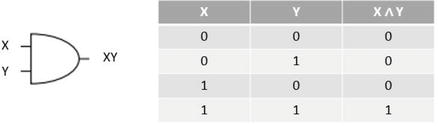
• AND gate output is going to equal $1$ when both input bits are $1$. It’s circuit and truth table are (Figure 1).

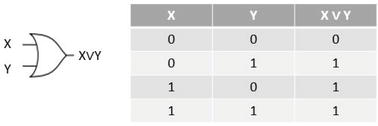
• OR gate output is going to equal $1$ if either of the input bits are $1$. It’s circuit and truth table are (Figure 2).

Figure 1.

Circuit diagram for the AND logical irreversible gate and the truth table.

Figure 2.

Circuit diagram for the OR logical irreversible gate and the truth table.

The OR gate, like the AND gate, is implemented in actual circuits using transistors and other electrical elements. Because the input states cannot be uniquely identified from the output, both the AND and OR gates are irreversible. In other words, if you know the result of an AND or OR gate, you cannot figure out what inputs produced that output. Reversible gates, on the other hand, allow for the complete recovery of input data from output data.

2.3 NAND and NOR: universal gates

In digital logic circuits, universal gates are ones that can be used to implement any other gate. The NAND gate and the NOR gate are two often used universal gates. NAND and NOR gates, as well as $\mathit{\text{AND}}$, $\mathit{\text{OR}}$, $\mathit{\text{NOT}}$, and $\mathit{XOR}$ gates, can be used to build any other gate.

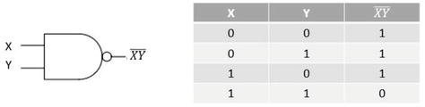
• NAND gate which stands for NOT of AND, and which outputs the NOT of the AND of the bits. It’s circuit and truth table are (Figure 3).

• NOR gate, which stands for NOT of OR, and which outputs the NOT of the OR of the bits. It’s circuit and truth table are (Figure 4).

Figure 3.

Circuit diagram for the NAND logical universal gate and the truth table.

Figure 4.

Circuit diagram for the NOR logical universal gate and the truth table.

The NAND gate is created by combining an AND gate and a NOT gate. It takes two binary inputs, X and Y, and outputs the logical inverse of the AND operation. If both inputs are $1$, the output is $0$; else the output is $1$. The NOR gate accepts two binary inputs, A and B, and outputs the logical inverse of the OR operator. Only if both inputs are $0$ is the output $1$; if not the output is $0$. Because of their versatility and ability to implement any other gate, NAND and NOR gates are frequently employed in digital logic circuits and computer architectures.

2.4 SWAP, NOT and CNOT: reversible gates

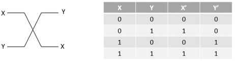
An even more complicated gate is SWAP gate, it is an exchange of bits (2 inputs, 2 outputs), it a common gate between classical and quantum computer, To generate the effect of a SWAP operation, some action has to take place. A SWAP gate icon that is more common in quantum circuit designs. The reason for having a different icon for SWAP in quantum circuits than in classical circuits is because many quantum circuit implementations do not have physical wires. As consequence, representing a SWAP operation as a wire crossing may be misleading. Instead, a SWAP operation can be accomplished using a number of applied fields (Figure 5).

Figure 5.

Circuit diagram for the SWAP gate and the truth table.

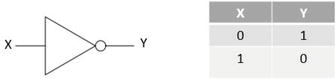
The NOT gate is often employed in classical computing for many kinds of functions such as logical operations, binary arithmetic, and controlling data flow in digital circuits. It is one of the fundamental components that are used in the making of more complicated logic circuits and computer systems. In computer programming, the NOT gate is also used to complement binary integers and execute bitwise NOT operations. The NOT Gate is a single reversible gate, it takes a single input bit and get a single output bit. If the input bit is $0$, the NOT gate outputs $1$, else it outputs $0$ (Figure 6).

Figure 6.

Circuit diagram for the NOT gate and the truth table.

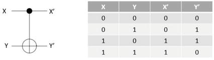
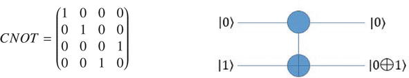
The Controlled-NOT (CNOT) gate is not a normal gate in classical computing like the AND, OR, or NOT gates, but its functionality can be resembled using other classical logic gates. The CNOT gate is a two-qubit gate that performs a controlled NOT operation on the second qubit dependent on the state of the first qubit in quantum computing. A combination of AND, OR, and NOT gates can be used to achieve the functionality (Figure 7).

Figure 7.

Circuit diagram for the CNOT gate and the truth table.

Although the classical CNOT gate, which is implemented using AND, OR and NOT gates can achieve functionality, as the CNOT gate it’s important to note that the classical implementation lacks reversibility. Reversible computing pertains to a concept where all operations and gates are designed in such a way that information can be accurately retrieved from the output. Unfortunately this classical CNOT implementation does not fulfill that requirement.

2.5 Is all Boolean circuits can be simulated reversibly?

On the side reversible computing is a type of computing approach that focuses on carrying out computations in a manner that preserves information. This means that the original inputs can be retrieved uniquely from the outputs. Reversible computing is closely tied to the concept of information conservation. Requires that the number of inputs, to a circuit matches the number of outputs. However traditional Boolean circuits used in classical computing suffer from information loss due to operations such as AND and OR gates [10]. These gates lead to information loss making it impossible to recover the inputs with certainty, from the outputs. Reversible computing is closely connected to information conservation, and the number of inputs to a reversible circuit must be the same as the number of outputs. Many Classical Boolean circuits used in classical computing, on the other hand, contain fundamental information loss due to irreversible operations such as AND and OR gates. These gates generate information loss, make it impossible to figure out the original inputs from the outputs in an unusual way. Consider a simple AND gate with two inputs A and B and a single output C. The output C is $1$, if both $X$ and $Y$ are $1$, and $0$ for all other input combinations. If we know $W$ is $0$, we cannot tell if $X$ and $Y$ were both $0$ or one of them was $1$ [11]. As a result of this, because information about the original inputs is lost, this AND gate is irreversible. Certain gates, such as the Controlled-NOT (CNOT) gate in quantum computing, are reversible and can be simulated reversibly. In quantum computing, the CNOT gate is usually used to implement reversible logic operations.

• Reversible simulation is impossible: If a Boolean circuit F is irreversible, at least one input combination $\left(X_i\right)$ gives the same output $\left(W_j\right)$ as another input combination $\left(X_k\right)$ giving the same output $\left(W_j\right)$. If $X_i$ $\ne$ $X_k$ exist such that $F\left(X_i\right)$ = $F\left(X_k\right)$ for some output index j $\left(W_j\right)$, then F is irreversible.

• Let us prove it by contradiction: Let us assume a reversible simulation of the irreversible circuit F exists. This reversible simulation would have created different results for all possible input combinations. However, because F is irreversible, there are input combinations $X_i$ and $X_k$ ($X_i$ $\ne$ of $X_k$) in which $F\left(X_i\right)=F\left(X_k\right)$. The reversible simulation cannot find $X_i$ and $X_k$ uniquely from the same output, which put us in a contradiction.

The bit is the smallest unit of classical information, with two possible states: 0 or 1. Information can be encoded using bits. Logic gates such as NOT, AND, OR, XOR, NAND, and NOR operate on bits. These gates, when we put them together, we are allowed do any computation, and combination of these gates, such as NOT, AND, OR, and NAND, that are also universal. Classical computers can handle some problems and calculations quickly, but others take a long time to find the solution, and it might be correct or faults. Some tasks that are difficult for classical computers, that’s why they are thought to be solved by quantum computers.

3. Quantum computing

After examining both irreversible and reversible gates we gained a deeper understanding of the advantages offered by quantum gates. In the domain of computation a series of logic gates operates on a limited number of classical bits at once. Similarly in quantum computation a sequence of quantum logic gates acts on a qubits at a time to represent the process. The primary difference is that classical logic gates manipulate classical bit values, either $0$ or $1$, yet quantum gates can manipulate complicated multi-partite quantum states, including arbitrary superpositions of computational base states, which are frequently entangled [12]. As a consequence, the logic circuits used in quantum computation have a much wider range of operations than those used in classical computation. At the present, certain industries are building quantum computers on a limited scale. The development of quantum computers confronts obstacles as the number of factors that influence their performance and limit their scale. To properly illustrate quantum characteristics, qubits must be maintained in a controlled environment where all qubits function in a correlated manner. Even tiny changes in the quantum system’s environment may perturb the qubits and even initiate a system crash. By following the laws of quantum physics, quantum computers present several states at once, and establish a vessel of correlation between them, which extremely enhances its processing powers [13].

3.1 Quantum dynamics

The Schrödinger equation is at the foundation of quantum dynamics, describing how the quantum state of a system grows over time [14]. It’s the basis of quantum mechanics and provides insights into the behavior of particles and wavefunctions. The time-dependent Schrödinger equation is given by

$$i\mathrm{\hslash }\frac{\partial }{\partial t}\mid \mathrm{\Psi }\left(t\right)⟩=H\mid \mathrm{\Psi }\left(t\right)⟩,$$E1

where $i$ represents the imaginary unit, $\mathrm{\hslash }$ denotes the reduced Planck constant, $\frac{\partial }{\partial t}\mid \mathrm{\Psi }\left(t\right)⟩$ signifies the partial derivative of the quantum state $\mid \mathrm{\Psi }\left(t\right)⟩$ with respect to $t$, and $H$ stands for the Hamiltonian operator, which encapsulates the total energy of the quantum system. In numerous instances, the Hamiltonian operator can be expressed as the combination of the kinetic energy $\left(T\right)$ and potential energy $\left(V\right)$ operators, i.e., $H=T+V$. The kinetic energy operator $T$ is derived from the momentum operator $p$ squared, divided by twice the mass $m$, thus yielding $T=p^2/2m$. Conversely, the potential energy operator $V$ hinges on the spatial coordinates of the system and represents the interaction energies within the system.

The time-dependent Schrödinger equation provides a mathematical framework to predict the future behavior of a quantum system, given its initial state and the Hamiltonian operator. Solving this equation allows us to determine how the quantum state $\mid \mathrm{\Psi }\left(t\right)⟩$ evolves over time. It’s important to note that the Schrödinger equation is a cornerstone of non-relativistic quantum mechanics. For relativistic particles, such as those moving at velocity close to the speed of light, a more comprehensive equation known as the Dirac equation is used. Solving the Schrödinger equation for complex quantum systems, especially those involving multiple particles, can be challenging. Numerical methods, approximations, and simplifications are often employed for getting insights into the behavior of quantum systems [15]. The Schrödinger equation captures the concept of quantum dynamics by characterizing the time evolution of quantum states in response to the Hamiltonian operator. It’s an effective equation that supports much of our understanding of quantum mechanics and plays a crucial role in fields that extend from atomic and molecular physics to quantum computing. The Schrödinger equation expand on its significance and dig into its mathematical form in more details, like the “wave function evolution” of a quantum system over time, while the wavefunction contains all the information about the quantum state, including the probabilities of various measurement outcomes, by solving the Schrödinger equation allows us to know how these probabilities vary in time. We have also the Superposition described by the Schrödinger equation, any system in quantum mechanics can exist in superposition, unless we disturb this superposition influencing the probabilities of various outcomes, and the Schrödinger equation explains how these superpositions evolve.

3.2 Quantum superposition

In the complicated field of quantum mechanics, a phenomenon known as superposition comes up as a remarkable characteristic that defies classical intuition. Superposition entails the difficult ability of quantum systems to exist in a variety of states simultaneously, confusing the conventional binary distinction. The Schrödinger equation, which we previously examined in greater detail, plays a pivotal role in describing the dynamics of superposition and offers a mathematical framework for comprehending the coexistence of multiple states within a single quantum entity [16]. This extraordinary trait introduces a profound shift in how we comprehend the fundamental constituents of the universe, driving us beyond classical boundaries into a domain where particles and systems can effectively traverse a multiplicity of potential states. As we begin on an exploration to learn about the complex nature of superposition, we will delve into its implications, manifestations, and the intriguing ways it intersects with the Schrödinger equation. Through this investigation, we will uncover the remarkable aspects of superposition that reveal the fascinating nature of quantum reality. As we explained previously the qubit is in a superposition, meaning that it can be in state $\mid 0⟩$ and $\mid 1⟩$ at the same time, we described by the follow equation:

$$\mid \mathrm{\Psi }⟩=\frac{1}{\sqrt{2}}\left(|0⟩+|1⟩\right)$$

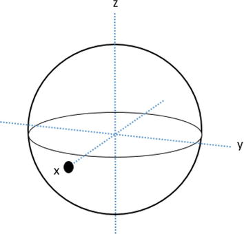
This exciting concept is beautifully captured by the Bloch vector, a pointer extending from the sphere’s center, which traces out the qubit’s trip through superposition [17]. The Bloch sphere offers an actual means to intuitively comprehend the complicity of probabilities that define superposition, providing both a theoretical framework and a geometrical sphere for investigating the remarkable nature of quantum states (Figure 8).

Figure 8.

Bloch sphere where the state is at the $\left(x,y,z\right)$ point $\left(\mathrm{1,0,0}\right)$, where the Bloch sphere intersects the $x$ axis.

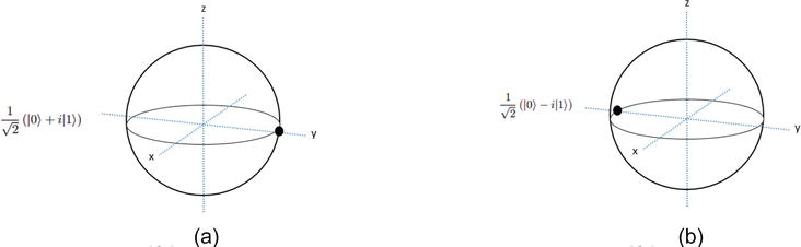
We can also demonstrate states with an imaginary and complex numbers that are used in quantum computing. In quantum mechanics, complex numbers provide an essential role in representing quantum states and transformations. When representing quantum states on the Bloch sphere, the horizontal angle corresponds to the phase of complex probability amplitudes. This phase, encoded in the complex numbers, contributes to interference phenomena and the observed probabilities of measurement outcomes. Moreover, the Bloch sphere’s vertical angle represents the probability amplitudes themselves, blending real and imaginary components to define the state’s position. Complex numbers introduce an additional dimension to the Bloch sphere, allowing us to obtain the full meaning of quantum superposition and entanglement. By adopting the mathematics of imaginary and complex numbers, the Bloch sphere in which we can determine the quantum states and provide behaviors of the quantum state (Figure 9).

Figure 9.

Bloch sphere where in $\left(a\right)$ the state is at the $y$ axis at point $\left(\mathrm{0,1,0}\right)$, in $\left(b\right)$ the state is at the $y$ axis at point $\left(0,-1,0\right)$.

In the domain of quantum physics, the Bloch sphere serves as a bridge between the abstract and the visual, giving a unique view into the quantum states behavior. Through its elegant representation, we open a better knowledge of superposition, entanglement, and the probabilities that include the quantum field. As we move the surface of the Bloch sphere, led by the mathematics of imaginary and complex numbers, we discover a dimension where particles may occupy several states simultaneously. This understanding helps us understand the significance of quantum sates. The Bloch sphere helps us see beyond the limitations of classical understanding.

3.3 Quantum entanglement

Entanglement, a phenomenon at the basis of quantum mechanics, is both mysterious and fascinating. It defines a unique state where the properties of two or more particles become correlated in such a way that their individual quantum states cannot be described independently [17]. Instead, they are intricately linked, regardless of the distance between them. This remarkable connection challenges our classical intuitions and has profound implications for our understanding of the nature of reality. Imagine two entangled particles, often referred to as “spooky action at a distance” by Einstein, Podolsky, and Rosen (EPR) in their famous thought experiment. When the quantum state of one particle is measured, the state of the other particle instantly “collapses” into a corresponding state, no matter how far apart they are. This instantaneous correlation defies our classical notions of causality and presents concerns about the true nature of information transfer in the quantum field. Entanglement is beautifully visualized in the context of the Bloch sphere. Imagine two entangled particles, each represented by a Bloch vector on its own sphere. These vectors are intrinsically linked such that if you measure the spin of one particle along a certain axis, the other particle’s spin will be immediately known along the same axis, regardless of the distance separating them. This phenomenon has significant practical implications, particularly in the emerging field of quantum computing and quantum communication. Entanglement functions as a resource to perform operations that are not classically possible, enabling quantum computers to potentially solve intricate problems at an exponential speedup compared to classical computers. Furthermore, entanglement-based quantum communication has the promise of secure communication protocols, where any spying would disrupt the delicate entanglement and thus be detectable [18]. Yet, entanglement also raises significant philosophical concerns about the nature of reality and how we fit in the universe. It challenges the notion of local reality, suggesting that our world may not operate according to the intuitive classical principles we have come to expect.

Let us proceed to the subject of entanglement using mathematics to get a more complete understand. Entanglement happens when two or more quantum systems become paired in such a way that their individual states cannot be represented separately [19]. Mathematically, let us imagine a system of two qubits, A and B. Their combined state, represented as a tensor product, can be stated as:

$$\left|{\mathrm{\Psi }}_{\mathit{AB}}\right.⟩=\alpha \left|0_A\right.⟩\otimes \beta \left|1_B\right.⟩-\beta \left|1_A\right.⟩\otimes \alpha \left|0_B\right.⟩$$E2

Here, $\alpha$ and $\beta$ are complex probability amplitudes, $\left|0_A\right.⟩$ and $\left|1_B\right.⟩$ represent the basis states of qubit $A$, and $\left|0_B\right.⟩$ and $\left|1_B\right.⟩$ represent the basis states of qubit $B$.

Bell states are unique entangled states with the strongest correlation. One such Bell state is the singlet state:

$$\left|{\mathrm{\Psi }}^{-}\right.⟩=\frac{1}{\sqrt{2}}\left(\left|0_A\right.⟩\otimes \left|1_B\right.⟩-\left|1_A\right.⟩\otimes \left|0_B\right.⟩\right)$$E3

When measuring the first qubit in the singlet state along the $Z$ axis (spin measurement), the second qubit’s state quickly collapses to the opposite consequence. If qubit A is measured as $\left|0\right.⟩$, qubit B will be $\left|1\right.⟩$, and vice versa. Mathematically, this could be written as: If $A$ is measured as $\left|0_A\right.⟩$, then $B$ is $\left|1_B\right.⟩$, and vice versa.

In the context of entanglement, the Einstein-Podolsky-Rosen (EPR) problem reveals the non-local character of quantum correlations. The EPR argument includes two entangled particles, A and B, in a singlet state $\left|{\mathrm{\Psi }}^{-}\right.⟩$. The spin measurements in a specified direction for each particle are characterized by operators $S_{\mathit{Az}}$ ad $S_{\mathit{Bz}}$, where $S_{\mathit{Ax}}$ denotes the spin operator for particle A along the x-axis. These operators have eigenvalues of $\pm \frac{\mathrm{\hslash }}{2}$, signifying the two probable results of measurement. The EPR argument focuses on the correlation between the measurements of particles A and B along the same axis. By measuring the spin of particle A along the x axis $S_{\mathit{Ax}}$ and particle B along the x axis $S_{\mathit{Bx}}$ gives us:

$$S_{\mathit{Ax}}\left|{\mathrm{\Psi }}^{-}\right.⟩=\frac{\mathrm{\hslash }}{2}\left|{\mathrm{\Psi }}^{-}\right.⟩,S_{\mathit{Bx}}\left|{\mathrm{\Psi }}^{-}\right.⟩=-\frac{\mathrm{\hslash }}{2}\left|{\mathrm{\Psi }}^{-}\right.⟩.$$E4

It means that if particle A is found with spin up in the x-direction, particle B will be found with spin down, and vice versa. This quick correlation across space, no matter the distance between the particles, is a key component of the EPR paradox and what Einstein referred to as “spooky action at a distance”. Bell’s inequality is an equation that quantifies the correlations predicted between measurements on entangled particles offered they meet local reality, a classical idea that argues that physical attributes are predetermined and do not change instantly. For a system including the measurement angles $\theta$ and $\varphi$ for particles A and B, Bell’s inequality is generally written as: $S\left(\theta ,\varphi \right)⩽2$, here, $S\left(\theta ,\varphi \right)$ is the correlation function that measures the correlation between the measurement outputs. If the measured correlation exceeds the value of 2, it indicates a violation of Bell’s inequality and suggests that the observed correlations cannot be explained by local realism. Experimental studies of Bell’s inequality have demonstrated violations, showing the non-local and non classical nature of entanglement. Violations of Bell’s inequality suggest that the entangled particles are connected in ways that cannot be explained by traditional physics (Figure 10) [20].

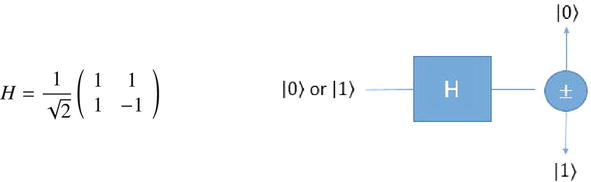
Figure 10.

Hadamard gate.

$$H=\frac{1}{\sqrt{2}}\left(\begin{array}{cc}1& 1\\ 1& -1\end{array}\right)$$

3.4 Pauli spin matrices

Pauli spin matrices are the mathematical tools in quantum physics that represent the fundamental momentum, or spin of particles, especially fermions like electrons. Expressed as matrices, these operators give an approach for expressing the spin states and interactions of particles [21]. The Pauli spin matrices, indicated by ${\sigma }_x$, ${\sigma }_y$ and ${\sigma }_z$, are fundamental for understanding different quantum system. They are defined as follows in their matrix form:

$${\sigma }_x=\left(\begin{array}{cc}0& 1\\ 1& 0\end{array}\right),{\sigma }_y=\left(\begin{array}{cc}0& -i\\ i& 0\end{array}\right),{\sigma }_z=\left(\begin{array}{cc}1& 0\\ 0& -1\end{array}\right)$$E5

These matrices describe spin observables along three orthogonal axes in a quantum system. When applied to spin $-1/2$ particles, like electrons, the Pauli spin matrices generate a set of eigenstates combining to the possible spin measurements in each direction. The commutation relations between these matrices show the non-commutative character of spin observables, which is a hallmark of quantum mechanics. The Pauli matrices find use in many different applications, from expressing spin states of particles to creating quantum gates in quantum computing. Their elegant matrix representations include the complex behavior of quantum spins, contributing significantly to the development and understanding of quantum mechanics [22].

Quantum gates are important in building blocks of quantum computing, letting the control and transformation of qubits, the basic units of quantum information. These gates are represented as unitary matrices which operate on the quantum state vector. Quantum gates perform a function similar to traditional logic gates, but with the extra complexity of superposition and entanglement. One of the most fundamental quantum gates is the Hadamard gate $\left(H\right)$, which creates superpositions between qubits, it is described by the matrix: We apply the Hadamard gate to qubits as follow:

$$H\left|0\right.⟩=\frac{1}{\sqrt{2}}\left(\left|0\right.⟩+\left|1\right.⟩\right),H\left|1\right.⟩=\frac{1}{\sqrt{2}}\left(\left|0\right.⟩-\left|1\right.⟩\right).$$E6

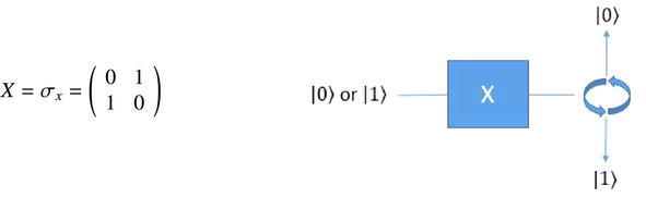
Another significant gate is the Pauli-X gate, ${\sigma }_x$, which performs a bit-flip operation, and the phase change is done by the Pauli-Y gate ${\sigma }_y$ and the Pauli-Z ${\sigma }_z$ gate. Quantum gates can be coupled to create complicated quantum circuits. For instance, the Controlled-NOT (CNOT) gate, a two qubit gate, flips the target qubit if and only if the control qubit is $\left|1\right.⟩$, and it is represented by the matrix: The application of quantum gates lets us create quantum algorithms and perform operations using the concepts of superposition and entanglement. These gates constitute the basis of quantum computing and provide the possibility for addressing difficult problems beyond the capability of classical computers. The Pauli-X gate ($X$ or ${\sigma }_x$) is a fundamental quantum gate that functions as a bit-flip operation, similar to the conventional NOT gate. Mathematically, the Pauli-X gate is represented by the matrix: we apply the X gate to the qubits as follow (Figures 11 and 12).

Figure 11.

The CNOT gate.

Figure 12.

the NOT gate.

$$\mathit{\text{CNOT}}=\left(\begin{array}{cccc}1& 0& 0& 0\\ 0& 1& 0& 0\\ 0& 0& 0& 1\\ 0& 0& 1& 0\end{array}\right)$$

$$X={\sigma }_x=\left(\begin{array}{cc}0& 1\\ 1& 0\end{array}\right)$$

$$X\left|0\right.⟩=\left|1\right.⟩)X\left|1\right.⟩=\left|0\right.⟩$$E7

In the Bloch sphere represented, the Pauli-X gate flips the quantum state vector across the x-axis. This gate is important because it puts the basis for quantum error correction, quantum cryptography, and is an essential component in several quantum algorithms [23]. By combining the Pauli-X gate with other quantum gates like the Hadamard gate, Pauli-Y gate, and Pauli-Z gate, we can create quantum circuits that execute complex operations on qubits. These gates, functioning in the domain of superposition and entanglement, allow quantum computers to deal with problems that are impossible for classical computers, offering a new generation of computing and scientific growth [24].

4. Quantum data compression

To begin, we’ll need a number that indicates how much knowledge you’d acquire if you knew the quantum state of some system. The Von Neumann entropy is an appropriate quantity [25]:

$$S\left(\rho \right)=-\mathit{Tr\rho }log\rho ,$$E8

where the trace operation and $\rho$ is the density operator characterizing a quantum system’s ensemble of states. This is in contrast to the traditional Shannon entropy.

$$S\left(\left\{p\left(x\right)\right\}\right)=-\sum _{x}p\left(x\right){log}_{2}p\left(x\right).$$E9

Assume that the probability distribution of a classical random variable $X$ is $p\left(x\right)$. The density matrix of a quantum system prepared in a state $\mid x⟩$ dictated by the value of $X$ is ${\sum }_{x}p\left(x\right)\mid x⟩⟨x\mid$, where the states $\mid x⟩$ need not be orthogonal. $S\left(\rho \right)$ is demonstrated to represent an upper limit on the classical mutual information $I\left(X:Y\right)$ between $X$ and the outcome $Y$ of a system measurement. We analyze the resources required to store or communicate the state of a quantum system $q^{\prime }$ of density matrix $\rho$ to create a link using qubits. The goal is to gather $n\gg 1$ of these systems and transmit the combined state into a smaller system. The smaller system is broadcast down the channel, and the combined state is decoded at the receiving end into $n$ systems $q$ of the same kind as $q$. Each $q$‘s final density matrix is ${\rho }^{\prime }$, and the entire process is considered successful if $\rho$ is sufficiently near to. The fidelity defined by is a measure of resemblance between two density matrices [26].

$$f\left(\rho ,{\rho }^{\prime }\right)={\left(\left(\mathit{Tr}\sqrt{{\rho }^{1/2}{\rho }^{\prime }{\rho }^{1/2}}\right)\right)}^2.$$E10

This can be read as the likelihood that $q$ will pass a test to determine if it is in the state $\rho$. The fidelity is none other than the classic overlap: $f={‖\phi ⟩⟨\phi ‖}^2$ when $\rho$ and ${\rho }^{\prime }$ are both pure states, $\mid \phi ⟩⟨\phi \mid$ and $\mid {\phi }^{\prime }⟩⟨{\phi }^{\prime }\mid$. The complete state of $n$ systems is represented by a vector in a Hilbert space of $2^n$ dimensions, if we limit ourselves to $2\mathit{\text{state}}$ systems for simplicity. If the Von Neumann entropy $S\left(\rho \right)⟨1$, the state vector is very likely to lie in a typical Hilbert space subspace in any given realization.

Moreover, the encoding and decoding operations are blind: they do not require knowledge of the precise states that are being communicated. The $\mathit{\text{encoding}}$ and $\mathit{\text{decoding}}$ necessary to produce such quantum data compression and decompression are technically challenging. It is currently impossible to do so using photons. It is, nevertheless, the maximum compression permitted by the rules of physics. Other classical notions like Huffman coding, as well as the fundamental concept of information, have quantum equivalents [27]. In addition, Schumacher and Nielson develop a number called “coherent information,” which is a measure of mutual information for quantum systems. It encompasses the portion of mutual information between entangled systems that cannot be accounted for using traditional methods. This is an excellent method to comprehend the Bell–EPR relationships.

5. Quantum information protocols

5.1 Quantum key distribution

Quantum cryptography is a branch of research that uses quantum mechanics principles to encrypt and transmit data so that hackers cannot access it. The development and execution of various cryptographic tasks using the unique capabilities and power of quantum computers are also included in the larger use of quantum cryptography. Quantum computers have the potential to help the creation of new, stronger, and more efficient encryption methods that would be difficult to create using current computing and communication infrastructures [28]. The following are two popular, although quite different cryptography applications that are being developed using quantum properties:

• Quantum key distribution: is the act of having a common key between two trusted parties utilizing quantum communication so that an untrusted “eavesdropper” cannot learn anything about the key.

• Quantum safe cryptography: is the development of cryptographic algorithms, also defined as post-quantum cryptography, that are secure against a quantum computer attack and may be used to provide quantum-safe certificates.

Quantum Key Distribution (QKD) entails transmitting encrypted data via networks as classical bits, while the keys to decode the data are encoded and sent as qubits in a quantum state. For implementing QKD, many methods, or protocols, have been devised. This is how BB84, a frequently used one, operates. Imagine Alice and Bob, two humans. Alice wants to transmit Bob info in a secure manner. To accomplish so, she builds a qubit based encryption key whose polarization states reflect the key’s individual bit values.

“Decoherence” will force some of the qubits’ delicate quantum states to collapse as they travel to their destination. To account for this, Alice and Bob do “key distillation,” which entails determining if the error rate is high enough to indicate that a hacker has attempted to intercept the key. If that’s the case, they discard the suspicious key and continue to generate new ones until they are certain they are sharing a secure one. Alice may then use hers to encrypt data and send it to Bob in classical bits, which he can decode using his key [29].

5.2 The BB84 protocol for distributing quantum keys

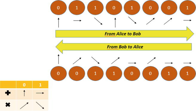
Charles Bennett and Gilles Brassard devised the first quantum key distribution technique in 1984, which is also known as BB84 [30]. The system is based on the dispersion of single photons or particles. The polarization of a photon will encode the value of a classical bit. We’d want to convey some facts about photons and the quantum mechanical description utilized in the protocol before we describe the BB84 system.

With quantum cryptography, the key is a stream of photons, photons have a property called spin that can be changed as soon as it pass by filter. We have two groups of filers rectilinear $\mid \uparrow ⟩$, $\mid \to ⟩$ and diagonal $\mid \nwarrow ⟩$, $\mid \nearrow ⟩$. The state of $\mid \to ⟩$ and $\mid \nearrow ⟩$ codes $1$ while $\mid \uparrow ⟩$ and $\mid \nwarrow ⟩$ codes $0$. Alice decides whether to encode her random number using a rectilinear or diagonal basis at random for each transmission. Each photon’s polarization is now picked at random from a set of ($\mid \uparrow ⟩$, $\mid \to ⟩$, $\mid \nwarrow ⟩$, $\mid \nearrow ⟩$), making it impossible for Eve to identify its polarization state. Because a $\mid \nwarrow ⟩$ or $\mid \nearrow ⟩$ polarized photon has the same chance of being projected into either horizontal or vertical polarization state (we call it a measurement in rectilinear basis), Eve will destroy information encoded in diagonal basis if she uses a polarization beam splitter to project the input photon into either horizontal or vertical polarization state (we call it a measurement in rectilinear basis). Eve and Bob are perplexed since none of them knows which basis Alice will pick ahead of time. Bob picks either a rectilinear or a diagonal basis to measure each incoming photon at random, unaware of Alice’s basis decision. Alice and Bob can create correlated random bits if they both utilize the same basis [31]. Their bit values, on the other hand, are uncorrelated if they employ distinct bases. After Bob has measured all of the photons, he uses an authorized public channel to compare his measurement bases with Alice. They only maintain sifting keys, which are random bits produced with matching bases. Their filtered keys are identical and may be utilized as a secure key without ambient sounds, system flaws, or Eve’s interference.

• Alice picks the basis and polarization of her photons at random and transmits them to Bob. She wishes to send a string of bits 110,101,101,001, for example. She will pick a basis (either horizontal or vertical) at random for each bit, as illustrated in 1.13.

• Bob picks a basis at random for each photon he receives and uses it to measure that photon. If he uses the same basis as Alice, he will get the same result, i.e. the interpreted bit will be accurate. If he picks a different foundation, though, he will get either 0 or 1 with equal likelihood. As a result, this is a completely random process in which some bits will be correctly translated while others will be incorrect. 1.13 depicts Bob’s measuring procedure and the bases he picked at random. A raw key is a series of interpreted bits like Bob’s. As a result, Alice’s raw key is the first set of bits she sent to Bob.

• Bob utilizes the public channel to communicate with Alice in order to figure out which parts he got right. He does not provide the measurement’s findings, i.e. the raw key, but rather the foundation on which each Alice’s photon was received. If Alice uses the same foundation for each photon, she will have an agreement with Bob. If Alice’s foundation differs from Bob’s, she declares a dispute. This may be seen in the image above. Both Alice and Bob then filter their raw keys to get a shorter sequence of bits called a sifted key by removing bits associated with unpleasant bases (Figure 13).

Figure 13.

Alice delivers the photons, which are all programmed on a random basis.

As a result, if Alice and Bob utilized the same basis for a photon, whether rectilinear or diagonal, they should have the same filtered keys. The filtered key, according to theory, will be the secret key. However, this is only true when dealing with a flawless experiment. In the actual world, the environment will alter the polarization of photons in optical fiber, or Eve will corrupt certain photons during eavesdropping owing to an incorrectly selected foundation. As a result, the filtered keys of Alice and Bob will not match, indicating that Eve is listening in. Alice and Bob pose the filtered keys, which are not equal in practice, after the three major phases of the BB84 protocol. In that case, a few more steps are required: estimation of the transmission error rate based on a random sample from both sides’ raw keys (random bits are then discarded from the raw keys); extraction of the reconciled key, i.e. error free common key, using some error correction methods; and, finally, privacy amplification, i.e. extraction of the reconciled key.

Other QKD methods follow the same stages as the ones we have listed here. EPR and B92 QKD methods are also available for information purposes only. The B92 protocol may be simplified to BB84, but the EPR procedure employs quantum-correlated particles, which are photon pairs created by certain particle processes. Various QKD protocols are given, as well as explanations of particular error correcting methods.

As we go further into the domain of quantum mechanics, we switch our focusing from the basic concepts of quantum gates and entanglement to study two events that demonstrate the unique character of the quantum universe. The first of these is the idea of non-cloning, a concept that contradicts standard concepts of replicating information. In the quantum domain, perfect copying of arbitrary quantum states is disallowed owing to the famous “no-cloning theorem,” which we shall unravel via its mathematical expression. Building upon this, we will next go into the interesting notion of quantum teleportation, a method that permits the transmission of quantum information from one point to another without physical movement. Through mathematical equations, we will explore the complicated mechanics behind these events and reveal the potential they provide in the field of quantum information [32].

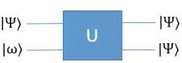
5.3 No-cloning

There is no unitary operator that can clone arbitrary qubit, unless the state has previously been determined. The unitary operator can be express as a circuit (Figure 14):

Figure 14.

Unitary operator circuit.

Where $\mid \omega ⟩=\mid 0⟩$, mathematically we can say $U\left(|\mathrm{\Psi }⟩|\omega ⟩\right)=\mid \mathrm{\Psi }⟩\mid \mathrm{\Psi }⟩$. Let us proof that cloning is not linear and hence cannot be unitary, We think about the situation $\mid \mathrm{\Psi }⟩=\mid \alpha ⟩+\mid \beta ⟩$, we have $U\left(|\mathrm{\Psi }⟩|0⟩\right)=\mid \mathit{\alpha \alpha }⟩+\mid \mathit{\beta \beta }⟩\ne \mid \mathrm{\Psi }⟩\mid \mathrm{\Psi }⟩$. Each particular cloning operation $U$ can work on certain states (in the case above $\mid \alpha ⟩$ and $\mid \beta ⟩$), but because $U$ is trace preserving, two clonable states must be orthogonal, $⟨\alpha |\beta ⟩=0$. When special relativity principles are addressed, EPR correlations might be used to communicate faster than light if cloning were possible. This would result in a contradiction; an effect before a cause [33].

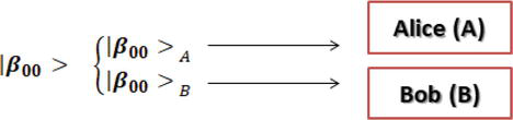
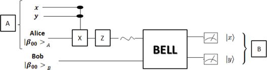
5.4 Super dense coding

Classical information may be stored and transmitted using qubits. Super dense coding unable us to have a powerful quantum communication, whereby it is possible to increase the information capacity of a link by transmitting two bits by sending only one qubit, this is only possible through the generation, manipulation and measurement of an entangled state [34, 35]. Alice ${}^{\text{'}}{A}^{\prime }$ can send Bob ${}^{\text{'}}{B}^{\prime }$ a single qubit across space (two classical bits for one qubit):

$$0=00$$

$$1=01$$

$$2=10$$

$$3=11$$

It take two ordinary bits; each probably consisting of servel thousand atoms)to express the same amount of informations. Alice ${}^{\text{'}}{A}^{\prime }$ can send Bob ${}^{\text{'}}{B}^{\prime }$ first prepare an entangled Bell state and each takes one qubit from that state, thus setting us their communication apparatus (Figure 15).

Figure 15.

The two halves of the entangled bell state’s creation and distribution.

When Alice is ready, she authors one of the four two bits messages, she then runs her entangled qubit; which is her half of Bell state; through a unitary logic gate $\left\{I,X,Y,Z\right\}$ which is determined by the message she wants to send. Alice ships her qubits off to Bob, who’ll have the complete $\mathit{\text{entangled}}$ bipartite state $\mid {\beta }_{00}⟩$ (the full entangled pair), with:

$$\mid {\beta }_{00}⟩=\frac{\mid 00⟩+\mid 11⟩}{\sqrt{2}},\mid {\beta }_{01}⟩=\frac{\mid 01⟩+\mid 10⟩}{\sqrt{2}},\mid {\beta }_{10}⟩=\frac{\mid 00⟩-\mid 11⟩}{\sqrt{2}},\mid {\beta }_{10}⟩=\frac{\mid 01⟩-\mid 10⟩}{\sqrt{2}}$$E11

Bob measures his bipartite state along the Bell basis. Which Bell gate is a combination of $\mathit{\text{CNOT}}$ and the first order $\mathit{\text{Hadamard}}$. Bob will get one of the four values. The resulting measurement will reveal the message. We can create a circuit for the superdense coding method as a whole:

• the transmission of traditional bits.

• Classical bits based on decisions.

• Communication between communicators is noiseless (Figure 16).

Figure 16.

The superdense coding circuit.

Alice controls (filled circles) which of the four operations (1, X, Z, or iY) she will perform to her qubit using her two-bit classical message $\mathit{xy}$. Bob measures both qubits along the Bell basis after transmitting her qubit to bob to retrieve the message $\mathit{xy}$, which is now sitting in the output registers in natural z-basis form $\mid x⟩,\mid y⟩$ .

5.5 Quantum teleportation

At the heart of quantum teleportation are two important principles: entanglement and quantum superposition. Quantum superposition, on the other hand, allows particles to exist in numerous states simultaneously, until a measurement collapses the superposition into a definitive state [36]. Quantum Teleportation is when Alice transmitted Bob one qubit, $\mid \psi ⟩=\mid 0⟩+\mid 1⟩$, in superdense coding to reassemble two classical bits. The mirror counterpart of this technique is quantum teleportation. Alice wishes to communicate Bob the qubit, $\mid \psi ⟩$, using only two traditional bits of information. Alice’s goal is to send to Bob a complete qubit, which contains a value that represents one of the infinitely possible superposition that can a state be in. The two prepare their communication channel by preparing their $\mathit{\text{Bell}}$ state, and each one is taking one components qubits. Next, Alice produces the general state $\mid {\psi }_c⟩$ for teleportation, but she has to get to Bob without sending the $\mid {\psi }_c⟩$, instead she feeds ket-psi along with her half of the Bell state into a binary gate, so Alice measure the output of that gate, she end up with one of four classical strings $\left(\mathrm{00,01,10,11}\right)$ [37, 38]. Alice sends her two classical bits to Bob; who uses them to decide how to process his half of entanglement Bell pair, after he does what the message instructs him to do, he got the original qubit,$\mid {\psi }_c⟩$. To explain more, Bob did not measure anything, he put his qubits through a binary gate, but the gate is unitary. Bob got his $\mid {\psi }_c⟩$ after receiving two measly classical bits [39]. The Quantum Teleportation process: it start with two entangled particles, generally identified as Alice and Bob. Additionally, Alice holds an additional particle called Charlie, meant to be teleportated to Bob. In this method, Alice makes a measurement involving her particle (Charlie) and the particle given for teleportation. Proceeding further, Alice executes a Bell measurement on her particles, gathering informations about the shared quantum state of the entangled particles—Alice’s and Bob’s; while avoiding direct measurement of their individual states. Following this, Alice uses classical communication to send the measurement result to Bob. The classical data comprises important characteristics about the original particle’s quantum state. Afterwards, Bob, informed by Alice’s classical knowledge, does certain quantum operations to his entangled particle. These operations bring about a transition in Bob’s particle, aligning it with the initial state of Charlie. With this manipulation finished, Bob’s particle successfully “mimics” the quantum state of the original particle, Charlie, eventually ending in the successful teleportation of its properties over space. Key Quantum Teleportation Protocols include the fundamental Original Protocol [40], which established the notion of quantum teleportation and proved the non-local transfer of quantum information. Additionally, the Dense Coding Protocol uses quantum teleportation principles to permit effective transfer of classical information via entangled particles. Cluster State Teleportation allows the teleportation of cluster states important in quantum computing, allowing distributed quantum computation. Finally, the Continuous Variable Teleportation protocol manages continuous quantum variables, such as quantum state phase and amplitude, allowing the development of high-capacity quantum communication channels.

5.5.1 Quantum teleportation implementation

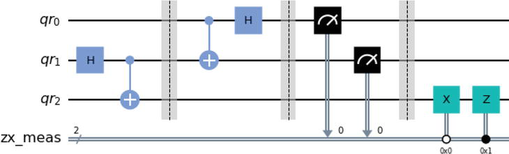
Quantum teleportation depends on the manipulation of quantum states through the application of quantum gates, which are basic operations that affect the state of a quantum system. These gates play an important part in preparing, entangling, and affecting the particles involved in the teleportation process. Let us examine how quantum gates are applied in quantum teleportation using a simple example in Qiskit, a common framework for quantum computing. Let us consider that Alice want to send to Bob an unknown state using bell state as an entangled state (Figure 17):

Figure 17.

Quantum teleportation circuit using bell state as entangled state.

The given Qiskit code generates and simulates a quantum circuit that includes many quantum gates and operations. We’ll break down the code step by step to understand it (Table 3).

Applications	Explanation
Importing Libraries	The code imports essential libraries
Quantum and Classical Registers	Registers for qubits and measurement.
Quantum Circuit Initialization	Called “circuit” formed with quantum and classical registers.
Hadamard Gate	Create a superposition between the qubits
Controlled-NOT Gate	CNOT gate entangles qubits; flips target if control qubit = 1
Barrier	separates circuit areas for improved clarity
Measurements	Qubits 0 and 1 measured, results in classical bits
X Gate and Z Gate	Conditional qubit operations based on classical measurements.

Table 3.

Explaining the use of the gate in the quantum circuit.

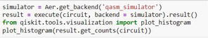
Beginning with the $\mathit{\text{Qasm}}$ simulator, the code goes as follows: The code is written in Qiskit, a quantum computing tool, to simulate and show quantum circuit results using a specific quantum simulator. Let us investigate the code’s parts and understand its purpose: To begin, the line “$\mathit{\text{simulator}}$ = $\mathit{Aer}.\mathit{\text{getbackend}}$($\mathit{\text{qasmsimulator}}$)” initializes a quantum simulator using Qiskit’s Aer backend. The $\mathit{\text{qasmsimulator}}$ backend simulates quantum circuit activity and estimates probability for different measurement results. Next, the code “$\mathit{\text{result}}$ = $\mathit{\text{execute}}\left(\mathit{\text{circuit}},\mathit{\text{backend}}=\mathit{\text{simulator}}\right).\mathit{\text{result}}\left(\right)$” uses the “execute” function to run the quantum circuit on the provided simulator backend (“simulator”). After that, by using the “$.\mathit{\text{result}}\left(\right)$” function, results can be obtained from the execution process. Moreover, the import phase here is “$\mathit{\text{from}}$ $\mathit{\text{qiskit}}.\mathit{\text{tools}}.\mathit{\text{visualization}}$ $\mathit{\text{import}}$ $\mathit{\text{plothistogram}}$” takes in the $\mathit{\text{plothistogram}}$ use from Qiskit’s visualization tools, allowing the creation of histograms that represent measurement results. In the end, the code provides a histogram plot using “$\mathit{\text{plothistogram}}\left(\mathit{\text{result}}.\mathit{\text{getcounts}}\left(\mathit{\text{circuit}}\right)\right)$”, offers a visual representation of the measurement results collected from the circuit performance. The $\mathit{\text{getcounts}}\left(\mathit{\text{circuit}}\right)$ function obtains result counts, and the “${\mathit{\text{plot}}}_h\mathit{\text{istogram}}$” tool shows these counts as a histogram. The second part of the algorithm includes determining outcome probabilities using the simulator (Figures 18 and 19).

Figure 18.

Outcome probability code of Qasm simulator.

Figure 19.

Outcome probability of Qasm simulator.

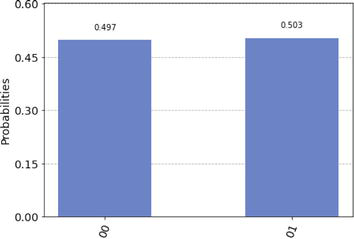
The resultant probabilities obtained from the executed quantum circuit represent the possibility of measuring the states. The circuit, including qubit gates and operations, creates probabilities for measuring varied qubit states. Breaking down the results for $00$ and $01$ states: For $00$, a probability of 0.497 corresponds to a 49.7 $\%$, the probability of measuring both qubits in state $\mid 0⟩$. In the case of $01$ the probability of 0.503 shows a 50.3 $\%$, the possibility of measuring the first qubit in state $\mid 0⟩$ and the second qubit in state $\mid 1⟩$. These probabilities replicate the behavior of the quantum circuit, created by applied gates and operations. Guided by quantum physics, measurement outputs are fundamentally probabilistic, their probabilities depending on qubit states during measurement [41].

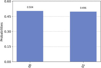
Similar behavior is seen in the Aer simulator, but with slightly different result of the outcome probability values. Next, we plot the $\mathit{\text{ibmqqasmsimulator}}$ (Figures 20–22):

Figure 20.

Outcome probability code of Aer simulator.

Figure 21.

Outcome probability of Aer simulator.

Figure 22.

Quantum teleportation circuit using bell state as entangled state.

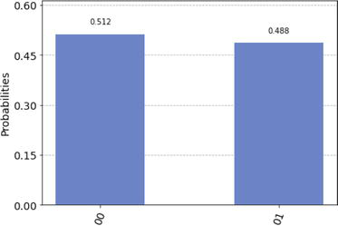
For the state $00$, the probability is 0.512 is 51.2 $\%$, the probability of measuring both qubits in the state $\mid 0⟩$. For the state $01$, the probability is 0.488 is 48.8 $\%$, the probability of measuring the first qubit in state $\mid 0⟩$ and the second qubit in state $\mid 1⟩$.

Comparing these results with the previous outcomes obtained from the Qasm simulator (for $00$ with probability = 0.497, and for $01$ with probability = 0.503) and the Aer simulator (for $00$, probability = 0.504, and for $01$, probability = 0.496), many observations can be made. The $\mathit{\text{ibmqqasmsimulator}}$ has a different probability distribution, showing changes in quantum behavior compared to both the Qasm and Aer simulators. The particular probabilities associated with each state vary by the simulator being used, reflecting the random character of quantum systems. The advantages of using the $\mathit{\text{ibmqqasmsimulator}}$ extend beyond basic result variations. This simulator is meant to exactly copy the behavior of real IBM Quantum devices, capturing real-world quantum effects and noise. Despite other idealistic simulators (such as the Qasm and Aer simulators), the $\mathit{\text{ibmqqasmsimulator}}$ gives a more realistic simulation that matches the settings of quantum computers. This allows researchers and developers to examine how quantum algorithms and circuits will work on real machines, perhaps exposing problems that are possible due to noise and other non-ideal conditions. Therefore, the $\mathit{\text{ibmqqasmsimulator}}$ serves as a helpful simulator for testing and improving quantum algorithms before deploying them on real quantum devices.

5.5.2 Bidirectional quantum teleportation (BQT) implementation

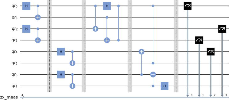
BQT is our approach includes the deployment of a Bell Quantum Teleporter (BQT), a conceptual construct that employs the quantum entanglement to perform teleportation by transferring two arbitrary quantum states in opposite directions. To assist this process, we use two pairs of Bell states, precisely prepared to encode and transport the quantum information. Furthermore, two Cluster states are brought forth, acting as the basic entangled states (Figure 23).

Figure 23.

Bidirectional quantum teleportation circuit using two bell states and two cluster states as entangled state.

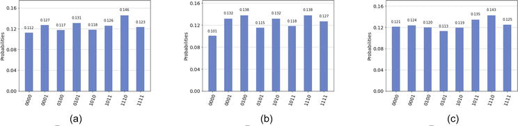
The code initializes the Qiskit environment and builds a quantum circuit named “circuit” with 8 qubits and 4 classical bits for measurement results. The quantum and classical registers are defined using the QuantumRegister and ClassicalRegister classes, respectively. we establish two Bell states using Hadamard (H) gates and controlled-X (CX or CNOT) gates. Bell states are maximally entangled quantum states. The first two qubits (qr[0] and qr.[1]) constitute the first Bell state, while the following two qubits (qr[2] and qr.[3]) form the second Bell state. Then we generated two cluster states, which are different quantum states with a special entanglement structure. In this example, the cluster states are produced using Hadamard (H) gates and controlled-X (CX) gates. For the example presented, the cluster states are assumed to be $\mid 00>+\mid 11>$. After then quantum teleportation happens from qubit 0 (sender) to qubit 4 (receiver). It includes a series of controlled operations, including controlled-X (CX) gates and controlled-Z (CZ) gates. Quantum teleportation allows the teleportation of quantum information from one qubit to another using entanglement. Then we conducts another round of quantum teleportation, this time from qubit 4 back to qubit 0. Similar controlled methods are utilized to achieve this teleportation. we apply operations Measurements to qubits 0, 3, 4, and 2, which correspond to the transmitter and receiver qubits. The measurement results will be saved in the classical registers cr[0], cr[1], cr[2], and cr[3]. In our case, when we plot and simulate the circuit using QASM, Aer, and the Belem simulator, we obtain good results describe the behavior of quantum teleportation and entanglement. Each simulator gives an individual perspective on how the quantum circuit operations establish, delivering significant information on the quantum states and measurement results. Here’s what we observe (Figure 24).

Figure 24.

Three separate quantum simulation perspectives: (a) the Aer simulator shows real-world noise affects, (b) the Qasm simulator reveals the ideal quantum teleportation process, and (c) the Belem simulator delivers advanced, high-fidelity insights.

The $\mathit{\text{Qasm}}$ simulator emulates quantum processes using a classical way, to study the optimal behavior of quantum circuits. When plotted in the Qasm simulator, the circuit show a clear sequence of gate operations, entanglement, teleportation steps, and measurements. The measurement outputs are probabilistic, reflecting the quantum nature of the system, but the simulation is not account for noise that genuine quantum hardware. The Aer simulator gives a more realistic simulation by integrating noise models and other non-ideal factors. When our circuit is plotted in the $\mathit{Aer}$ simulator, we detect further fluctuations in the measurement outputs because of simulated noise. This provide us information into how noise affects the teleportation process. The $\mathit{\text{Belem}}$ simulator is especially built to deliver accurate quantum simulations using high-performance computer resources. When visualizing the circuit in the Belem simulator, we get an exact simulations that shows from the results a complicated interactions between qubits and complex noise models. This simulator provide us a complete knowledge of how the circuit operate on complex quantum systems, delivering insights into possible obstacles and improvements required for real-world implementation.

6. Closing remarks

From classical computation to quantum computation, we have begun on the possibility of changing our understanding of computing power and information processing. Through this study, we have exploited the power of quantum physics to show how we went from classical computers paradigm their challenges to quantum computing. By applying Qiskit platform, we managed to explain the basics of building a quantum teleportation circuit as an example, which has enabled us to experience quantum entanglement in action. Through precisely controlled procedures and measurable consequences, we have proven the teleportation of information between qubits, overcoming physical barriers in a manner that conventional communication could never do. In the context of bidirectional quantum teleportation, the difficulties of sending and receiving quantum states have been released, showing the complication of Bell states and cluster states that support this amazing phenomenon. Quantum computers interact and cooperate in ways that give us the results fast and more accurate. The achievements gained with Qiskit open the door for a quantum revolution that might influence industries ranging from encryption to optimization and drug discovery. By understanding the basic principles of quantum physics and applying the power of quantum gates and entanglement, we begin to find the transformational powers of quantum computers. With Qiskit as our guide, the road from classical to quantum computing becomes an exciting adventure in defining the future of technology and science.

References

1.Bremner MJ, Jozsa R, Shepherd DJ. Classical simulation of commuting quantum computations implies collapse of the polynomial hierarchy. Proceedings of the Royal Society A Mathematical, Physical and Engineering Sciences. 2011;467:459-472
2.Montanaro A. Quantum algorithms: An overview. NPJ Quantum Information. 2016;2:1-8
3.Aaronson S, Chen L. Complexity-theoretic foundations of quantum supremacy experiments. arXiv preprint arXiv:1612.05903. 2016
4.Williams CP, Clearwater SH. Explorations in Quantum Computing. Santa Clara: Telos; 1998
5.Knill E. Quantum computing. Nature. 2010;463:441-443
6.Ladd TD, Jelezko F, Laflamme R, Nakamura Y, Monroe C, O’Brien JL. Quantum computing. Nature. 2010;464:45-53
7.Canteaut A, Videau M. Symmetric boolean functions. IEEE Transactions on Information Theory. 2005;51:2791-2811
8.O’Donnell R. Some topics in analysis of Boolean functions. In: Proceedings of the Fortieth Annual ACM Symposium on Theory of Computing. 2008. pp. 569-578
9.Steane A. Quantum computing. Reports on Progress in Physics. 1998;61:117
10.Steane A. Quantum computing. Reports on Progress in Physics. 1998;61:117
11.Keyl M. Fundamentals of quantum information theory. Physics Reports. 2002;369:431-548
13.Aharonov D. Quantum computation. Annual Reviews of Computational Physics VI. 1999;1999:259-346
14.Erdős L, Schlein B, Yau HT. Derivation of the cubic non-linear Schrödinger equation from quantum dynamics of many-body systems. Inventiones Mathematicae. 2007;167:515-614
15.Ollitrault PJ, Miessen A, Tavernelli I. Molecular quantum dynamics: A quantum computing perspective. Accounts of Chemical Research. 2021;54:4229-4238
16.Grover LK. Synthesis of quantum superpositions by quantum computation. Physical Review Letters. 2000;85:1334
17.Khrennikov A. Roots of quantum computing supremacy: Superposition, entanglement, or complementarity? European Physical Journal Special Topics. 2021;230:1053-1057
18.Preskill J. Quantum computing and the entanglement frontier. arXiv preprint:1203.5813. 2012
19.Sørensen A, Mølmer K. Entanglement and quantum computation with ions in thermal motion. Physical Review A. 2000;62:022311
20.Raussendorf R, Wei TC. Quantum computation by local measurement. Annual Review of Condensed Matter Physics. 2012;3:239-261
21.Patera J, Zassenhaus H. The Pauli matrices in n dimensions and finest gradings of simple lie algebras of type a n–1. Journal of Mathematical Physics. 1988;29:665-673
22.Briegel HJ, Browne DE, Dür W, Raussendorf R, Van den Nest M. Measurement-based quantum computation. Nature Physics. 2009;5:19-26
23.Mosseri R, Dandoloff R. Geometry of entangled states, Bloch spheres and Hopf fibrations. Journal of Physics A: Mathematical and General. 2001;34:10243
24.Mäkelä H, Messina A. N-qubit states as points on the Bloch sphere. Physica Scripta. 2010;2010:014054
25.Yu CH, Gao F, Lin S, Wang J. Quantum data compression by principal component analysis. Quantum Information Processing. 2019;18:1-20
26.Legeza Ö, Sólyom J. Quantum data compression, quantum information generation, and the density-matrix renormalization group method. Physical Review B. 2004;70:205118
27.Dilip R, Liu YJ, Smith A, Pollmann F. Data compression for quantum machine learning. Physical Review Research. 2022;4:043007
28.Gisin N, Ribordy G, Tittel W, Zbinden H. Quantum cryptography. Reviews of Modern Physics. 2002;74:145
29.Zhang Q, Yin J, Chen TY, Lu S, Zhang J, Li XQ, et al. Experimental fault-tolerant quantum cryptography in a decoherence-free subspace. Physical Review A. 2006;73:020301
31.Shor PW, Preskill J. Simple proof of security of the BB84 quantum key distribution protocol. Physical Review Letters. 2000;85:441
32.Bennett CH, DiVincenzo DP. Quantum information and computation. Nature. 2000;404:247-255
33.Jaeger G. Quantum Information. New York: Springer; 2007. pp. 81-89
34.Harrow A, Hayden P, Leung D. Superdense coding of quantum states. Physical Review Letters. 2004;92:187901
35.Zhao J, Jeng H, Conlon LO, Tserkis S, Shajilal B, Liu K, et al. Enhancing quantum teleportation efficacy with noiseless linear amplification. Nature Communications. 2023;14:4745
36.Mafi Y, Kazemikhah P, Ahmadkhaniha A, Aghababa H, Kolahdouz M. Bidirectional quantum teleportation of an arbitrary number of qubits over a noisy quantum system using 2n bell states as quantum channel. Optical and Quantum Electronics. 2022;54:568
37.Kirdi ME, Slaoui A, Hadfi HE, Daoud M. Improving the probabilistic quantum teleportation efficiency of arbitrary superposed coherent state using multipartite even and odd j-spin coherent states as resource. Applied Physics B. 2023;129:94
38.Kirdi ME, Slaoui A, Hadfi HE, Daoud M. Efficient quantum controlled teleportation of an arbitrary three-qubit state using two GHZ entangled states and one bell entangled state. Journal of Russian Laser Research. 2023;44:121-134
39.Legeza Ö, Sólyom J. Optimizing the density-matrix renormalization group method using quantum information entropy. Physical Review B. 2003;68:195116
40.Bennett CH, Brassard G, Crépeau C, Jozsa R, Peres A, Wootters WK. Teleporting an unknown quantum state via dual classical and Einstein-Podolsky-Rosen channels. Physical Review Letters. 1993;70:1895
41.Ikken N, Slaoui A, Laamara RA, Drissi LB. Bidirectional quantum teleportation of even and odd coherent states through the multipartite Glauber coherent state: Theory and implementation. arXiv preprint:2306.00505. 2023