Perspective Chapter: The Proton’s Theoretical Description, Based on Wigner-Segal Approach to Elementary Particles

Abstract

The chapter focuses on the Multi-Level Model (MLM), a conceptual framework proposed by Levichev. The essence of the MLM is the amalgamation of Segal’s chronometry and the Standard Model (SM), a fundamental theory in particle physics. The potential applications of MLM in proton therapy are predicated on the concept of the infinite-dimensional space denoted as F_p, encompassing the entirety of proton wave functions. The inherent properties of F_p-elements f are outlined. This analysis then proceeds to capture distinct instances (“snap shot photos”) of these functions at the temporal instant t = 0. The corresponding graphical representations of these functions are elucidated using precise geometric terminology. Specifically, two distinct types of graphs are identified: ND) a bell-shaped surface lacking a central depression, and WD) a bell-shaped surface featuring a central dent. In an endeavor to establish a connection between these mathematical revelations and proton therapy dosimetry, the exploration delves into a comparison of various classes of functions f from F_p with those produced within diverse proton therapy vaults. This integration proposes the incorporation of a novel ingredient into dosimetry, namely, the incorporation of the proton’s wave function. This innovative approach holds promise for refining proton therapy techniques and enhancing treatment precision.

1. Introduction

In accordance with the tenets of the Standard Model (SM), a proton p is postulated to consist of two u-quarks and one d-quark. Experimental evidence, particularly the detection of three distinct point-like centers through highly inelastic electron-proton scattering [1], substantiates this structural characterization of the proton. To elaborate on quark-gluon interactions, the Multi-Level Model (MLM) was introduced in Ref. [2]. Although Refs. [2, 3] have defined MLM-gluons, no subsequent developments have been pursued in this direction, making a discussion of gluons superfluous for our present topic. However, it is relevant to recall a fundamental conjecture derived from Refs. [2, 3]: (1) Free gluons manifest as detectable photons. An analogous conjecture pertaining to quarks is posited [2, 3]: (2) Free quarks materialize as protons (or antiprotons). Regarding the latter, this chapter aims to present a robust theoretical foundation, as demonstrated below in a significant portion of our content. Our treatment of the well-known SM-quarks is outlined in Section 3.

The core focus of our chapter is the exploration of the chronometric proton—a term whose implication will be clarified. While our examination predominantly revolves around this, it is important to acknowledge the involvement of other fermions such as quarks and leptons. Our overall goal also involves establishing a more rigorous foundation for the above second conjecture. Commencing with the upcoming section, we revisit the foundational principles and terminology of MLM (largely referencing [2, 3]). In our endeavor to mathematically characterize elementary particles, we employ Segal’s Chronometric Theory. Notably, Section “Indecomposable Elementary Particle Associations” in Ref. [4]—effectively summarizing Segal’s findings—holds a key role, and readers are advised to have this concise 5-page paper accessible as we delve into Chronometry-related aspects. The approach presented in Refs. [4] can be perceived as a generalization of Wigner’s proposal [5] to model particles through specific representations of the Poincaré group, denoted as P. Intriguingly, Segal [4] delves into specific representations of G = SU(2,2), often referred to as the conformal Lie group. This group is characterized by the 4 by 4 diagonal matrix S with entries 1, 1, −1, −1. The group G encompasses 4 by 4 matrices g (with complex entries) satisfying both a determinant one condition and the equation

$$g^{\ast }\mathit{Sg}=S,$$E1

where g^* is the transpose and complex conjugate of g. G encompasses the extended (by scaling) Poincaré group P+ and its subgroup P, which are both 11-dimensional and 10-dimensional, respectively. The essence of Chronometry is deeply rooted in the (acclaimed!) linear-fractional G-action on the unitary group U(2), elucidated in Appendix A. For a comprehensive understanding of Segal’s compact cosmos D, readers are directed to the inception of Section 2. Notably, the universal cover of D is fundamentally linked to the (renowned!) Einstein’s static universe, with its three-space representation encapsulated by SU(2). In Ref. [6], the approach introduced in Ref. [4] was coined as the Wigner-Segal method, propounding a unique methodology to model elementary particles.

Overall, this introduction sets the stage for our comprehensive exploration, encompassing the SM, MLM, and Chronometry, as we endeavor to elucidate the intricate fabric of elementary particle dynamics.

In Refs. [2, 3], the MLM was introduced as a potential alternative to the SM. After further investigation (see [6, 7, 8, 9, 10, 11, 12]), it has become evident that the MLM can now be understood as a fusion of Segal’s chronometry with the SM. The term “chronometric” highlights our engagement with chronometry (with its 15-dimensional core symmetry group G, as mentioned earlier). It is worth comparing the particles proposed by this theory with their relativistic counterparts, where the central symmetry group is the (10-dimensional) Poincaré group P—a fundamental player in relativistic physics. Just a reminder, the SM primarily addresses relativistic particles. In Ref. [3] (Section 2), there is a discussion of how certain traits of a chronometric particle can be interpreted within the context of relativity.

The chronometric proton p is elemental and unbreakable (so confinement is not a concern). We are fully aware that this assertion might ruffle feathers among many in the Physics community. Nevertheless, the MLM does not discard quarks entirely.

Specifically, in Refs. [2, 3], for each U(n) level where n > 2, the MLM-quark (with a specific flavor and color) was defined as a structured trio (D_pq, G_ij, m). Here, m can be either 1 or − 1, depending on whether it is a particle or an antiparticle. The subgroup D_pq within U(n) determines flavor, while the subgroup G_ij within SU(n,n) determines color. An implicit aspect of this definition involves a clearly defined representation space H, where the quark’s wave function finds its home. The governing group G_ij operates within this space.

The above paragraph has been extracted from the heart of Section 3 (sandwiched between Propositions 2 and 3) and placed here in the Introduction to offer a glimpse of what is to come for curious readers. But there is more: We interpret each MLM-quark q as a “captured proton,” and q’s electric charge can be either 1 or − 1. Now, what about the widely accepted fractional electric charges of SM-quarks? We see this as more of an artifact—a somewhat misleading or perplexing interpretation of data.

Speaking of the representation space H mentioned earlier, it is intricately defined by the comprehensive collection F_p of chronometric proton’s theoretically possible wave functions. This F_p was established in Ref. [11] and is discussed across Sections 2 (toward the end), 3, and 4.

2. From chronometry to the MLM-quarks of the U(3)-level

Mathematically, chronometry deals with a slightly larger totality of space–time events than the Minkowski space–time M has. Namely, the compact chronometric world D (or the Segal’s compact cosmos), as a manifold, is the unitary group U(2). This group is defined as the totality of all two-by-two matrices z (with complex entries allowed) satisfying

$${\mathit{z}}^{*}\mathit{z}=1,$$E2

where 1 is the unit matrix. Here (and on), we use world as a synonym of space–time. For our purposes, it suffices to stay with U(2), which is a compact manifold. To eliminate closed time-like loops, which are unavoidable when the world is compact, one has to move to the universal covering. It is well known that D is a natural alternative of M, the unique four-dimensional manifold with comparable properties of causality and symmetry. Free particles are considered to be associated with positive-energy representations in bundles of prescribed spin over D of the group of causality-preserving transformations and with corresponding wave equations.

The imbedding of M into D via the Cayley transform is well known, see formula (5.2) of [13]. The Lorentzian metric (or inner product) in D was introduced by Segal (and is given in Section 3.1 of [13]). This metric is left-invariant as well as right-invariant on the Lie group U(2). It is the authors’ strong belief that for the adequate understanding of the chapter, there is no need to explicitly write down this metric here. Recall that the above mentioned Poincare group P is the totality of all isometries of the (pseudo-Euclidian) M.

The main group of (causal) transformations in D is G = SU(2,2); in our Appendix A, we choose a generic element g₂ of SU(2,2) and we reproduce its action on a generic element z of D=U(2). It is the linear-fractional action.

When one switches to (an earlier mentioned) D’s universal cover, one has also to switch from SU(2,2) to its universal cover. In this regard, we only mention that there is a canonical mathematical way of treating such a situation: when (an arbitrary group) G acts on U, then there is a canonical action of the G’s universal cover on the U’s universal cover. In our presentation, it is enough to stay with G = SU(2,2) and with its linear-fractional action on D.

Certain representations (see [4]) of SU(2,2) give rise to chronometric particles, but we notice, once and for all, that we only need to deal with just one particular representation, the spannor one: It is discussed below.

Other details on chronometry can be found in Section 2 of Ref. [3]. As it follows from [11], certain corrections (of what Segal claimed in [4], and what was reproduced from [4] in Section 2 of [3]) are to be made. The research [11] can be viewed as a discussion of, and supplement to, Segal’s list of chronometric elementary particles of spin 1/2 [4]. The last article is in some sense a summary of Segal’s findings, and it is just 5 pages long. In Ref. [4], there are few, if any, clues of how to obtain results outlined in it. In publication [11], one of the main goals was to prove (some of) Segal’s statements. The most remarkable of these is that there are four elementary chronometric particles of spin 1/2. Namely, there is a massive neutral particle named the exon, the electron e, and two types of neutrino (interpreted as υ_e and υ_μ). The authors of Ref. [11] failed to prove that (but see what is said right below). In Segal’s theory, a particle (e.g., each of the above) is mathematically associated with an irreducible unitary positive-energy representations of the symmetry group G (in our case, the conformal group SU(2; 2)). Below, we associate certain mathematical objects with specific particles; Doing so, we try to stay in line with what Segal has done before in this regard. Here is the only significant exception to the above: around 2010 A. Levichev suggested in Ref. [14], Section 7, that it is rather the proton p than a hypothetical neutral particle, the exon.

Levichev’s Multi-Level Model of quarks, MLM [2, 3] claims that each SM-quark can be viewed as a “sunken (i.e., submerged) proton.” From Ref. [11], there is just one neutrino, rather than two, as in Ref. [4].

An earlier conjecture by Segal (about the number of chronometric spin 1/2 particles) was in compliance with the findings in Ref. [11], see [15] (Th. 16.7.10) that worked with a 3-step composition series. The spannor representation is a limiting case of representations studied by Jakobsen in Ref. [14], where, purely algebraically, a 3-step series may be obtained after the fact. Later, Segal’s original (i.e., the one of [15]) conclusion has been withdrawn: Table 1 of Ref. [4] states (without proof) the existence of the 4-step composition series. Overall, the authors of Ref. [11] follow the approach of Ref. [4]. Below (in this Section), we give more details from Ref. [11]. In the general context of how to mathematically define the notion of an elementary particle, we comment there on the transition from the renowned Wigner method to (what was called in Ref. [6] as) the Wigner–Segal method. From Ref. [11], there is a certain (infinite-dimensional) Hilbert space F_p (of functions on the Minkowski space–time M) that is interpreted as the set of all (theoretically possible) states (i.e., wave functions) of the chronometric proton p (see formula (20) of [11] and Theorem 3.1 of [10]). (More details on the space F_p are given in our Section 4.) The group G = SU(2,2) acts on F_p. According to the terminology of Ref. [10], Remark 4.1, this G is the ruling group, G_r, since it rules (or governs) the behavior of the particle.

As a mathematical model, MLM deals with the sequence of canonical (i.e., based on principal minors of the matrices involved) embeddings of groups: U(2) into U(3), U(2) into U(4), U(2) into U(5), and so forth. Each of these embeddings is an isomorphism onto the corresponding subgroup. These isomorphisms play an essential role on how to relate our MLM-quarks to the SM-quarks (for a quicker understanding of the MLM, go to Figure A1 of the Appendix A in [12]). The above groups were called levels: U(2) is the 0th level; U(3), the 1st; U(4), the 2nd; and so on. In Ref. [12], Section 3, it is shown that such a convention matches the standard quarks’ generations’ list. Recall that each matrix group U(n) is defined quite similarly to how U(2) was defined by our Eq. (2). Embeddings A₁₂, A₁₃, A₂₃ of (the Segal’s compact cosmos) D = U(2) into U(3) were introduced as follows: Under each of these three embeddings, a matrix Z from D becomes a certain principal 2 by 2 minor of the corresponding 3 by 3 matrix from U(3). Namely, denote by D₁₂ the image of the embedding A₁₂. The A₁₂, itself, is defined right below (also, these embeddings are illustrated in the top portion of Figure A1 of the Appendix A in Ref. [12]).

Each Z from D is put as an upper 2 by 2 principal minor of the 3 by 3 matrix A₁₂(Z) in U(3); the third diagonal entry of A₁₂(Z) is 1; in the A₁₂(Z), any other entry is zero. The two remaining embeddings, A₁₃ and A₂₃, are defined quite similarly. Clearly, D₁₂, D₁₃, and D₂₃ are U(2)–subgroups in U(3). Obviously, the group U(2) is closed with respect to the complex conjugation, and with respect to. the matrix transposition. The transposed matrix Z^T is obtained from Z by reflection in the principal diagonal. Hence, each of the D₁₂, D₁₃, and D₂₃ is invariant with respect to any of the two mentioned operations in U(3). Also, to enumerate all D_ij, it is enough to consider the cases i < j, only. Each D_ij carries a Lorentzian metric by the demand that each A_ij be an isometry.

In the totality of all m by m matrices, P_m is introduced, as the symmetry with respect to the opposite diagonal. Clearly, when Z is in U(2), then P₂(Z) is also in U(2). From this, it follows that the subgroup D₁₃ is P₃-invariant in U(3) while P₃(D₁₂) = D₂₃, P₃(D₂₃) = D₁₂. That enables us to view the embeddings A₁₂ and A₂₃ as equivalent (one becomes the other when composed with P₃ and P₂—see Figure A1 of the Appendix A in [12]). This relates to the “presence of two SM-u-quarks in” a proton, while the A₁₃ relates to the presence of an SM-d-quark in that proton. These embeddings make it possible to introduce a notion of a flavor of any MLM-quark of level U(3). The last two phrases are “nonmathematical;” we relate to physics here. We discuss this in more detail later in this section (right after Theorem 1).

Definition 1. Let us use the name cell for each of these D_ij.

It should always be stated (or should be clear from the context) which U(n)-level such a cell is considered to be in.

In Ref. [3], Section 3, similar to the way of introducing in U(3) of the U(2)-subgroups D₁₂, D₁₃, and D₂₃, the SU(2,2)-subgroups G₁₂, G₁₃, and G₂₃ of SU(3,3) have been defined. In our Appendix A, G₁₂ and G₁₃ are presented graphically. Namely, a generic element (of each of the two subgroups) is explicitly shown there. At each level U(n), any subgroup G_ij is defined in Section 4 of Ref. [12] (right before Proposition 2 there)—quite similar to how it has been done for the U(3)-level.

Definition 2. Let us use the name ruling (i.e., governing) group, or the r-group, for each of these G_ij (the latter being an SU(2,2)-subgroup of SU(n,n), in general).

It should always be stated (or should be clear from the context) which U(n)-level such an r-group is associated with. From Ref. [6], we now reproduce the following statement.

Theorem 1. An action of each of the subgroups G₁₂, G₁₃, and G₂₃on any of the subgroups D₁₂, D₁₃and D₂₃is defined. In particular, each of the following three actions, G₁₂on D₁₂, G₁₃on D₁₃, and G₂₃on D₂₃, is the linear-fractional one.

What about the mathematical meaning (and about the physical interpretation) of the following phrase (from above): “The embeddings A₁₂ and A₂₃ relate to the presence of two SM-u-quarks in a proton, while the A₁₃ relates to the presence of an SM-d-quark in that proton”?

According to the SM, a proton consists of two u-quarks and of one d-quark. The detection of three point-like centers (of highly inelastic electron-proton scattering, see [1]) served as an experimental basis for such a conclusion about the structure of a proton. However, after several decades of intense search, the majority of the Physics community has submitted to the view that “free quarks cannot be detected.”

Above, we have been discussing chronometric particles of spin 1/2. They originate from an induced representation of the group G = SU(2,2) defined by formula (5) from Section 2 of Ref. [11]. In Ref. [11], three chronometric spin 1/2 fermions have been mathematically detected: proton p, electronic neutrino υ_e, and electron e. On the basis of formula (16) from Ref. [11], the space F of the induced representation (sometimes referred to as the spannor representation, see [16]) of the group G = SU(2,2) has been introduced. In F, there exist two nontrivial invariant subspaces with no invariant complement. One of those subspaces was denoted by F_p, and it was supplied with a Hilbert space structure. On the basis of the findings in Refs. [17, 18], the following statement has been proven (see Section 5 of [11]):

Theorem 2. The restriction of the induced representation to F_pis unitary and irreducible. In F_p, the energy-positivity condition holds.

The space F_p has been interpreted as the totality of all (theoretically possible) wave functions of the chronometric proton. Notice that F_p is of conformal weight (or conformal dimension) 5/2, see Ref. [11].

Remark 1. Let us repeat that in Ref. [11], it was stated that F_p does not have an invariant complement. It means that we deal with the case where the Wigner method is not applicable. According to the Wigner-Segal method, introduce the quotient space W = F/F_p and the factor-representation in it. In Section 6 of Ref. [11], a minimal nontrivial invariant subspace F_υ in W has been supplied with the unitary structure and it has been interpreted as the totality of all wave functions of the chronometric electronic neutrino. In Ref. [11], Section 7, the quotient space W/F_υ = F_e has been interpreted as the totality of all wave functions of the chronometric electron (since the corresponding factor-representation turned out to be irreducible and unitarizable, and the conformal weight is 3/2 now). This was the final step in the proof of the main finding of Ref. [11]: There are exactly three elementary chronometric spin 1/2 particles.

Remark 2. Having in mind Remark 9.1 of Ref. [11], from now on, it seems plausible to associate the Hilbert space F_υ with the electronic antineutrino, rather than with electronic neutrino. The authors of Ref. [11] followed Segal (see [4]), and they interpreted this (“middle”) sector of the 3-step composition series as the one corresponding to the electronic neutrino, but (also in [11]) they have envisaged a possibility of the antineutrino interpretation. Such an interpretation can serve as a mathematical reason allowing a return (as it has been claimed in [19]) to an “old model” for the neutron as consisting of a proton, of an electron, and of an electronic antineutrino—see the U(2)-part of the Figure A4 (in the Appendix A of [12]).

For the level U(3), clearly, each A_ij is an isometry, and each D_ij is a space–time isometric to the Segal’s compact cosmos D. From here (and on the basis of both the above Theorem 2 and of its interpretation), we conclude that a spin 1/2 fermion (“living in” D_ij) is mathematically defined. If D₁₂ or D₂₃ is a support of its wave functions, then, as part of the MLM-settings, we associate this fermion with an u-quark. If D₁₃ is such a support, then the particle is interpreted as a d-quark. It means that in the MLM, we have introduced two flavors for quarks of the 1st level, U(3), and (by merely keeping the SM-terminology) we have established the correspondence of MLM-quarks to the SM-quarks, and vice versa. The Hilbert structure in the corresponding spaces H_ij is introduced via the isometries A_ij from the original H = F_p. For each of our fermions of the level U(3), its ruling group G can be any of G₁₂, G₁₃, or G₂₃. Such a convention was a mathematical basis for defining the notion of a color of an MLM-quark (see Sections 3 and 4 of [6], as well as our Section 3, below). Clearly, each MLM-quark is as fully described as the chronometric proton was—see our Theorem 2, above. We are thus able to interpret each MLM-quark q as a “captured proton”: a certain G_ij is its ruling group and q stays within the U(3) level.

Back to the highly inelastic electron-proton scattering: as the result of it, proton gets (from U(2)) to a “deeper” level, U(3). In U(3), it gets to one particular cell (of the total of three available ones: D₁₂, D₁₃, or D₂₃), thus “becoming an MLM-quark”. In terms of Physics, a possible description (see our Section 3, below) could use the following wording: our proton pushes “deeper” (i.e., to the U(4)-level) the “former occupant” of this cell. However, to better understand such a wording, one has to read our Section 3 first.

Since Ref. [12] has introduced equivalence (w.r.t. operators P₃ and P₂—see Figure A1 of the Appendix A there) between D₁₂ and D₂₃, we only have two flavors rather than three. In a formal agreement with the SM, our description of the highly inelastic scattering is that of the elastic one, but on quarks (in our case, on MLM-quarks). In particular, within the U(3) level, we should use another Hilbert space and another r-group.

Figures B1–B4 (of our Appendix B) show what specific geometric properties a proton’s wave function might have (= “what our proton might look like”). Seemingly, the thus suggested description of the highly inelastic electron-proton scattering does not, per se, contradict to detection, [1], of “three point-like components in a proton.” Also, in the MLM-approach, one can directly apply the combinatorial SM-methods to calculate relations between certain scattering probabilities. As an example ([12], p. 6), it is demonstrated that the ratio of (full) cross sections between πp- and pp-scatterings is in compliance with the SM-approach (while the latter fits experimental findings). Since (below) we discuss the “submerged vs. captured” proton, let us mention that Figures B1–B3 are indicative of the case of a captured proton while Figure B4 is of the submerged one.

3. An overview of the SM-quarks’ generations and the introduction of the MLM-quarks at “deeper” levels

Let us continue with more MLM-details. If our proton gets into the cell D₁₂, then we have to exploit the space F₁₂ of wave functions defined on D₁₂, rather than on the original D. Due to the isometry A₁₂ between D and D₁₂, the Hilbert spaces F_p and F₁₂ are unitarily equivalent. In Ref. [6], the notation q(1;1,2) has been used for such an MLM-quark: the first “1” is the level number (i.e., the U(3) level), while the pair (1,2) specifies the cell as D₁₂. Denoting the embeddings of D=U(2) into U(4) as A₁₂, A₁₃, A₁₄, A₂₃, A₂₄, and A₃₄ (see Figure A2 of Appendix A in [12]), the notation mimics the one already used in the U(3)-case. To determine equivalences, consider the operator P₄: the symmetry with respect to the opposite diagonal. Clearly (as Figure A2 of [12] illustrates), A₁₂ is equivalent to A₃₄, and A₁₃ is equivalent to A₂₄. Each of the subgroups D₁₄ and D₂₃ is P₄-invariant. Relate A₁₄ to an SM-quark s and A₂₃ to an SM-quark c. At this (i.e., at the second) level, A₁₂ (which is equivalent to A₃₄) relates to an SM-quark u, while A₁₃ (equivalent to A₂₄) relates to an SM-quark d. Hence, SM-quarks of both generations (one and two) “live” on the 2nd MLM-level, U(4).

Now, proceed with an overview of the SM-quarks’ generations, as well as of the topic in general. According to http://phys.vspu.ac.ru/forstudents/TSOR/Kutseva/pokolenie_leptonov_i_kvarkov.html, by 2018, it was known that there exist (at least) three generations of quarks and three generations of leptons. These fundamental particles are thought to be adequately modeled as the “point-like” ones. Both quarks and leptons have spin 1/2, which means that they are fermions. By convention, a fermion is a particle with half-integer spin, while a boson is a particle with an integer spin. Mathematically, a spin of a particle is a certain constant that is present in the (describing this very particle) representation of the group G—see, for instance, p. 348 of Ref. [20]. By G here (as well as above), we mean the main group of transformations acting in the space–time that our particle “lives in.” The word generation is part of the SM-terminology; generations will be naturally “built into” the MLM—see below. For other necessary details about fermions and of their role as seen by the SM, see Section 3 of [12]. The MLM-description of higher (than U(4)) level quarks is also given in that Section 3. From there, we only reproduce the following.

Remark 3. The SM-quarks of higher generations were detected later than SM-quarks of lower generations: with the increase of the accelerators’ typical energies. Hence, it is natural to interpret the “deepening,”, as n gets larger, of the U(n)-levels as corresponding to the increase of the scattering typical energy.

From [2, 3], reproduce Theorem 3.

Тheorem 3. On the level U(n), suppose an U(2)-subgroup D_ijbe not P_n-invariant. Then, D_ijcorresponds to a quark from a lower level. The recurrent (3) and explicit (4) formulas (for the total number m_nof quarks at the U(n)-level) hold:

$${\mathrm{m}}_2=1,{\mathrm{m}}_{\mathrm{n}}={\mathrm{m}}_{\mathrm{n}-1}+\left[\mathrm{n}/2\right],$$E3

$${\mathrm{m}}_{\mathrm{n}}=\left\{\mathrm{n}\left(\mathrm{n}-1\right)/2+\left[\mathrm{n}/2\right]\right\}/2.$$E4

Here, [x] denotes the greatest integer part (“roof”) of a real number x. We are thankful to the reviewer of [12] who has noticed that (4) can be simply expressed as [n²/4].

The “selection criterion” (i.e., why are we quite satisfied with our list of MLM-quarks) is the one that establishes their explicit correspondence with the SM-quarks. In levels U(3), U(4), and U(5), the MLM-quarks are in precise correspondence with the SM-quarks as they are currently agreed upon. In level U(6), three new SM-quarks are predicted, as illustrated by Figure A3 [12].

On p. 8 of Ref. [12], right after Remark 5 there, the color of an MLM-quark D_sk was defined as G_ij (which can be chosen from G₁₂, G₁₃, G₂₃). In other words, the color of an MLM-quark is defined by the choice of its ruling group (or, even more formally, the color (as a symbol) of an MLM-quark is (the symbol of) its ruling group). Recall that the ruling group also acts in the Hilbert space of wave functions of the quark in question (compared to what we have stated earlier, right after Remark 2). Clearly, there are three colors for quarks of the U(3)-level.

Now, let us introduce the notion of a color for an arbitrary U(n), with the integer n no less than 3. Given an embedding A_ij of D = U(2) into U(n), by G_ij, we understand a certain, uniquely defined SU(2,2)-subgroup in G_n = SU(n,n). Namely, G_ij consists of certain matrices g_n, uniquely defined by four n by n blocks A_n, B_n, C_n, and D_n. These four blocks are uniquely defined by the matrix g₂ (chosen arbitrarily) from G₂ = SU(2,2); in particular, G_ij is isomorphic to SU(2,2)—see Proposition 2, below. To continue, g₂ is determined by its 2 by 2 blocks A₂, B₂, C₂, D₂. To define n by n blocks A_n, B_n, C_n, D_n for g_n, proceed as follows (also, see our Appendix A). The block A_n is defined according to (1) and (2): (1) A₂ is that very minor in A_n; (2) any other entry in A_n is 1 (if on the principal diagonal) or it is zero (if it is off the principal diagonal)—compared to how G₁₂ was defined in our Section 2. The block D_n is defined quite similarly but with the help of D₂. The two remaining blocks, B_n and C_n, are defined (in terms of B₂ and C₂) somewhat differently. Namely, each entry, which is off the corresponding 2 by 2 principal minor of the block, is zero. The following statement has been proven in Ref. [3].

Proposition 2. G_ij is a subgroup of G_n; G_ij is isomorphic to SU(2,2).

In Refs. [2, 3], for each level U(n), with n greater than 2, the MLM-quark (of a certain flavor and color) was defined as an ordered triple (D_pq, G_ij, m). Here m is either 1 or negative 1 (depending on whether we deal with a particle or with an antiparticle). The subgroup D_pq in U(n) determines flavor, while the subgroup G_ij in SU(n,n) determines color. An implicit part of this definition is a well-defined representation space H, which the quark’s wave function belongs to. The ruling (i.e., governing) group G_ij acts in this H.

The following statement has been proven in Ref. [3]:

Proposition 3. The total number of colors at the U(n)-level is n(n-1)/2.

According to the SM (with its total number of colors being 3), the electric charge of each quark u (or c, or t) is 2/3, while the electric charge of each quark d (or s, or b) is minus 1/3. There is an approach with integer quarks’ electric charges [21]. Such an approach is known as the Han-Nambu scheme (in [21], there is a reference to the original Han-Nambu publications). Part of the Section 4 (in [12]) deals with an adaptation of the Han-Nambu scheme to the MLM.

Starting with the U(3)-level, here is the following possible interpretation in terms of physics: when a proton (participating in highly inelastic scattering) “finds itself” in a D₁₃-cell (and it stays there for a moment, name it a submerged proton), then its color may be one of G₁₂, G₂₃, or G₁₃ but changing between them with huge speed, presumably. A. Levichev likes a comparison with a “hot potato scenario” here: It is hardly possible to hold a hot potato in just one hand! Substitute “potato” by “proton” and “a hand” by “a ruling group.” The total number of ruling groups of the level U(n) increases as n gets larger. As stated in the Table 1 of Ref. [12], in D₁₃, these ruling subgroups generate electric charges 0, 0, negative 1, in that order. It means that a quark d has an average charge of negative 1/3. Similarly, a u-quark has charge 2/3. Notice that (from now on), we use submerged instead of sank (which appeared in [3]). As regards an electric charge generated by the ruling group, more details are provided in subsection 6.2 of [12].

On the basis of our Remark 2, above, and of the suggested MLM- approach to the values of SM-quarks’ electric charges, the following conjecture is logically noncontradictory:

Conjecture 1. The electric charges of the proton and of the electron (both viewed either “inside” neutron, or separately) originate as the result of the corresponding action (in their Hilbert spaces F_p and F_e) of the ruling group G (represented, essentially, by SU(2,2))_.

This (“philosophical”) view might serve as an answer (preliminary, at least) to the question “What are the origins of electric charge?” According to the SM (as well as to the MLM), there are color charges, too. Is it possible to interpret the chronometric proton’s electric charge as a special case of the MLM-quarks’ color charges? In the U(2)-level, there is just one ruling group for the proton, which means that there is just one color. Can we interpret this color charge as the electric charge of the chronometric proton?

The number of colors (in a given MLM-level) is level-dependent (see Proposition 3, above). In the U(5)-level, the electric charge values of MLM-quarks (in the “sunken proton” situation) are (slightly) different from those of the corresponding SM-quarks—see ([12], Section 4). Clearly, detection of this discrepancy might be a challenge for the current experimental physics!

In Section 5 of Ref. [12], the compilation of fermion triplets across levels U(2) through U(5) offers valuable insights into the potential structure of matter at deeper MLM-levels. Could the detection of hadron jets possibly serve as an indicator of this intriguing “MLM-structure”? It is plausible that this structure could undergo local disruptions during high-energy interactions, providing a more reasonable explanation than those proposed by the Standard Model. In this context, A. Levichev recollects his astonishment while navigating through PDG-files (available at http://pdg.lbl.gov/2018/reviews/rpp2018-rev-structure-functions.pdf). In Section 18.4, he encountered the term “hadronic structure of the photon,” a phrase that left a lasting impact. It is his aspiration that within scientific and medical circles, the prevailing perspective would lean toward regarding both photons and protons as elementary particles.

Concluding this section, we offer additional MLM-related insights, some in support, while others point out specific challenges and potential directions for future research.

Remark 4. The chronometric interactions are mathematically classified by Segal in Ref. ([4], p. 996). Before we implement his findings into the MLM-scheme, we need to double-check the constituents of the chronometric bosonic sector. As regards the MLM-Lagrangian, the challenges “hide” in the chronometry, already. Here is what Segal ([4], p. 995) said in this regard: “The elementary particles in chronometric theory are closely integrated into coherent entities …”, he calls them clans, “… Scalar, spinor, and vector elementary particles arise as subunits, and the fundamental interaction is between fermion and boson clans as entities, the total interaction Lagrangian being representable as a sum of interactions between individual elementary particles only in the relativistic limit.” The (mathematically pretty “delicate”) notion of the conformal weight plays the key role in classifying fundamental chronometric interactions: ([4], pp. 996, 997). As it has been detected in Ref. [11], the chronometric neutrino is not a particle of a certain conformal weight. This puts us in front of a new challenge: one has to modify, at least, the just mentioned Segal’s classification of chronometric interactions.

Figure A3 in Ref. [12] illustrates the MLM’s U(6)-level, and it suggests “where” to search for the (three) SM-quarks of the 4th generation—another challenge for the SM-experimental quest.

Overall, to the key MLM-conjecture, [12], that “an SM-quark can be interpreted either as a sunken or as a captured proton,” our chapter provides additional arguments. Unfortunately, we are not yet in a position to better support a claim of [3]—“At each level, a gluon can be interpreted as a colored and flavored photon,” since in order to do that, we have to start with a check of the bosonic sector findings by Segal. Recall that in Ref. [11], a similar check has been performed for the fermionic sector. Nevertheless, even at this point in time, it seems appropriate to mention the following chronometric findings: the key bosons (photon γ, W-boson, Z-boson) have been mathematically detected [4]. As regards the Higgs boson, on p. 996 of [4], Segal indicates the absence of one. To our mind (due to what we have above said), the Higgs boson existence stays as an open (mathematical) MLM-question, so far.

4. On the proton’s wave function and on its real-valued analogue

So far, the proton’s wave function in the literature (which we have had a look at) was treated in terms of proton’s quark constituents, like in https://physics.stackexchange.com/questions/2786/visualization-of-protons-wavefunction and in https://www.physicsforums.com/threads/do-protons-and-neutrons-have-a-wavefunctions.243322/.

Our view on proton is different, see the Introduction where the totality of its wave functions has been denoted as F_p and later, in Section 2 (Theorem 2), main properties of F_p have been stated. Right now, we provide more details on F_p.

In Ref. [11], the Minkowski space–time M is represented as a certain set of 2 by 2 matrices; let us use h to denote such an element (= event) in M:

$$\mathbf{h}=\left[\begin{array}{cc}{\mathit{x}}_{\mathrm{0}}+{\mathit{x}}_{\mathrm{1}}& {\mathit{x}}_{\mathrm{2}}+\mathit{i}{\mathit{x}}_{\mathrm{3}}\\ {\mathit{x}}_{\mathrm{2}}-\mathit{i}{\mathit{x}}_{\mathrm{3}}& {\mathit{x}}_{\mathrm{0}}-{\mathit{x}}_{\mathrm{1}}\end{array}\right].$$E5

In (5), above, real numbers x₀, x₁, x₂, x₃ are (standard) coordinates of the event in question; we say standard, meaning the case when M is presented as a four-dimensional vector space with a Lorentzian metric. It follows from Ref. ([11], eq. (20)) that each value of the proton’s wave function Ψ at h is the following vector in a complex 2-dimensional linear space C²:

$$\mathbf{\Psi }\left[\mathbf{w},\mathbf{v}\right]\left(\mathbf{h}\right)=\mathit{K}\left(\mathbf{h},\mathbf{w}\right)\mathbf{v}$$E6

By w*, below, we denote the matrix obtained from w by transposition and complex conjugation; w, above, belongs to a certain class of 2 by 2 matrices (see [11], Section 4). In the above (6), the notation Ψ[w,v] presumes that the wave function is defined as soon as the parameters w and v are chosen; here, v is from C². Also, the reproducing kernel K in (6) is defined by

$$\mathit{K}\left({\mathbf{w}}_1,{\mathbf{w}}_2\right)={\left\{\left({\mathbf{w}}_1-{{\mathbf{w}}_2}^{\ast }\right)/\left(\text{2i}\right)\right\}}^{-1}\{det[{\left\{\left({\mathbf{w}}_1-{{\mathbf{w}}_2}^{\ast }\right)/\left(\text{2i}\right)\right\}}^{-2},$$E7

where w₁, w₂ are taken from the abovementioned class of 2 by 2 matrices. It is well-known that expression (7) is always mathematically meaningful.

Essentially, we have thus introduced an (infinite-dimensional) Hilbert space F_p (of functions on the Minkowski space–time M), which is interpreted as the set of all (theoretically possible) states (or wave functions) of the chronometric proton p. This F_p is the completion of the span of the set of functions (6). The positive definite inner product <.,. > in F_p is defined as follows:

$$<{\mathbf{\Psi }}_{1,}{\mathbf{\Psi }}_2>=<\mathit{K}\left({\mathbf{w}}_1,{\mathbf{w}}_2\right){\mathbf{v}}_1,{\mathbf{v}}_2>,$$E8

where, in the right side of (8), the canonical inner product in C² is meant. As it has been stated in our Theorem 2, the restriction of the induced representation to F_p is unitary and irreducible. Here, the Mackey’s concept of induced representation is meant. This concept proved to be a major tool in the modern quantum mechanical description of a particle (see [20]). We apologize to the reader that the abovementioned representation (which is known as the spannor representation [4, 16]) cannot be fully described in our current text. We only recall that it is induced from a certain finite-dimensional representation of the (extended by scaling, and thus being 11-dimensional) Poincare group.

Using eq. (15) of [11], we have:

$$\mathrm{L}\left(\mathbf{h}\right)=\mathrm{SAv},$$E9

with always defined

$$\mathrm{S}={\left\{det\left[\left(\mathbf{h}–\mathrm{w}\right)/\left(\text{2i}\right)\right]\right\}}^{-2}.$$E10

Introduce the (real-valued!) function f as follows:

$$\mathrm{f}\left(\mathbf{h}\right)={\mathrm{L}}^{\ast }\mathrm{L},$$E11

where (for brevity) in the right side, we omit the argument h. To word it differently, the value of f at h is the Hermitian square of the vector in the right side of (6). From now, and till the end of Section 4, we refer to (11) as to the proton’s wave function. The expression for the 2 by 2 matrix A is (reproduced from [22]) as follows:

$$\mathrm{A}=\text{2i}{\left(\mathbf{h}–{\mathbf{w}}^{\ast }\right)}^{-1}.$$E12

In publication [22], the entries in (5), (9), and (10) have been specified as follows: x₀ = x₁ = 0; components of vector v: v₁ = 0, v₂ = 1; w = $\left[\begin{array}{cc}1+i& -1\\ -1& 1+i\end{array}\right]$. This results in h = $\left[\begin{array}{cc}0& z\\ \overline{z}& 0\end{array}\right]$ with z = x + iy. It means that in (5), we have simplified x₂ to x and x₃ to y. In our Appendix B, we thus deal with the real-valued function f(x,y). Here, x and y are the “usual” coordinates on the plane, while the remaining two coordinates (time t and the third space coordinate) are chosen as 0. In other words, it is the case of a “toy proton”; it was a first try (see [22]) to understand what kind of functions might be there, in the proton’s Hilbert space F_p. Dropping a (positive) constant factor, we end up with f(x,y) = ((x + 1)² + y² + 2)λ⁻³ where λ = ((x + 1)² + y²)² + 4. It turns out that f(x,y) has just one local minimum, at (−1,0) as shown on Figure B1. The totality of all points where f(x,y) reaches its maximum V is a circle defined by the equation (x + 1)² + y² = r². The radius r of this circle is determined from the system of equations for critical points of f(x,y). The highest points of the graph (as shown on Figures B2 and B3) form a circle that lies in the U = V plane; here, U is for the third coordinate in 3-space where we plot (portions of) the graph of f(x,y). The findings are graphically presented: Figures B1–B3. It is a bell-shaped surface with a dent on top. Clearly, it is important to move from this toy example to a more realistic one where f depends on all three space variables—we will refer to this case as to a “realistic proton,” see below. Notice that, obviously, f(h) in (11) is positive. We continue to refer to such an f(h) as to the “proton’s wave function” (despite a formal contradiction of (11) with formula (6), from above)—compared to how we have put it in Section 4 title: its real-valued analogue. When we allow for the third spatial dimension z, staying with the same v and with the same w, the result is as follows.

Тheorem 4. The resulting proton’s wave function is given by

$$\mathrm{f}\left(\mathrm{x},\mathrm{y},\mathrm{z}\right)=\left({\left(\mathrm{x}+1\right)}^2+{\mathrm{y}}^2+{\left(\mathrm{z}-1\right)}^2+1\right){\mathrm{\lambda }}^{-3},$$E13

where λ = ((x + 1)² + y² + z²)² + 4. As a 3-dimensional surface in R⁴ (with a ‘vertical’ coordinate U), the graph

$$\mathrm{U}=\mathrm{f}\left(\mathrm{x},\mathrm{y},\mathrm{z}\right),$$E14

is a bell-shaped surface E (with no dent on top). The highest point of E corresponds to the input (−1,0,z₁) where z₁is the (only!) real root of 5z⁵ – 11z⁴ + 12z³ – 4z + 4 = 0. Numerically, z₁is close to negative 0.65. The point (−1,0,z₁) is the center of our (realistic) proton.

Remark 5. Due to the chapter space limitation, we are unable to present all the details of the Theorem 4 proof. The plot of E’s typical section by a “vertical” 3-plane through the highest point of E is given by Figure B4. Not all cuts of E by U = const 3-planes are spheres (compared to a “toy proton” wave function where all of its graph cuts by horizontal 2-planes were circles).

Clearly, when z = 0 is entered into (13), we get our f(x,y), from above. That is, when we cut E by z = 0 3-plane, the result is a bell-shaped 2-surface with a dent on top.

Consider the following function:

$$\mathrm{g}\left(\mathrm{x},\mathrm{y},\mathrm{z}\right)=\left({\left(\mathrm{x}+1\right)}^2+{\mathrm{y}}^2+{\mathrm{z}}^2+2\right){\mathrm{\lambda }}^{-3},$$E15

with λ = ((x + 1)² + y² + z²)² + 4. Here is the equation of its graph J with such a (“desired”) spherical symmetry (w.r.t. the cuts by U = const 3-planes) property:

$$\mathrm{U}=\mathrm{g}\left(\mathrm{x},\mathrm{y},\mathrm{z}\right).$$E16

Obviously, the cut of J by the z = 0 3-plane is exactly the 2-dimensional surface shown on Figures B1–B3. It is so, since the input of z = 0 into (15) results in f(x,y) for the “toy proton”, from above.

Also, it is not difficult to show that J is a bell-shaped surface with a dent on top. Does g(x,y,z) originate from an element of F_p via formula (11)? It is an open question, so far.

5. Conclusion

As highlighted in the Introduction, the logical sequence of this chapter unfolds as follows. Our foundational cornerstone, serving as both our starting point and robust theoretical basis, is the MLM-theory, at times referred to as a fusion of Segal’s chronometry with the Standard Model. From the MLM perspective, protons emerge as the fundamental elementary particles of the natural world, supplanting the prominence of SM-quarks. This audacious assertion naturally necessitates a broader inclusion of mathematical descriptions for other essential particles, recognizing the significance of interactions in the grand scheme. In Sections 1 through 3, we establish essential mathematical frameworks and concepts, subsequently delving into a multitude of MLM-related applications and interpretations within the realm of Physics. All these endeavors have been distilled succinctly, with the intention to persuade the reader that a proton, in isolation, can, from the MLM standpoint, encompass the ability to model every current physical phenomenon explained through SM-quarks. Our modeling framework introduces novel concepts, including the notions of a sunken or submerged (“pritoplennyi” in Russian) proton, a captured proton, and the concept of the ruling group.

Only after we have navigated through a range of specific MLM-discoveries and challenges from a panoramic theoretical stance (particularly evident starting from Conjecture 1 and continuing through the culmination of Section 3), do we find ourselves suitably poised to revisit the crux of the matter—the chronometric proton itself. In Section 4, we dive deeper into the intricacies of F_p, the aggregate of its wave functions. While earlier, in Section 2 (Theorem 2), we established fundamental properties of F_p, our primary aim in Section 4 was to capture a snapshot of the proton’s wave function at the temporal juncture t = 0 and subsequently elucidate its corresponding graph through precise geometric terms. In a partial success (refer to Section 4 for comprehensive details), it appears we have managed to discern at least two distinct types of graphs, reflective of “members” within F_p: A) ND-case, a bell-shaped curve without a dent at its peak, and B) WD-case, a bell-shaped curve featuring a central dent. It is tentatively proposed that the ND-case corresponds to a submerged proton, while the WD-case corresponds to a captured proton, influenced by a specific ruling group.

While our journey to connect these findings with proton therapy dosimetry is still a work in progress, it is important to acknowledge the timeline of our key papers—[11, 12, 22]—which were recently published in 2022. We anticipate a surge of research contributions on this topic, especially after the publication of this book featuring our chapter. Moving forward, we outline potential avenues of exploration in the subsequent section, marking out the trajectories for future research endeavors.

6. Could our discoveries find relevance in the domain of proton therapy dosimetry?

Admittedly, it might seem a stretch to envision a direct application of our deeply theoretical and mathematically intricate proton description to practical medical contexts. Nevertheless, let us contemplate this within the realm of proton therapy.

Throughout our chapter, spanning from its inception and threading through the theoretical exposition of the chronometric proton, and further into Section 4 with its specific revelations, the spotlight remains firmly on the concept of the wave function. However, the question of whether the wave function possesses a tangible existence and what it truly signifies continues to loom large within the framework of quantum mechanics. This quandary has bewildered many prominent physicists, in the past and present. Notably, a substantial contingent of experts—though perhaps not the dominant majority—aligns with our standpoint: that the wave function must indeed possess an objective and physical reality. This perspective opens the door to exploring correlations between our findings and distinct designs of proton vaults.

Consider the scenario where diverse proton vaults give rise to proton beams of varying configurations. Within this context, our focus narrows in on the intriguing prospect of classifying these beams and subsequently linking them to distinctive characteristics of the proton’s wave function. Unfortunately, this promising avenue of research, aimed at applying our insights to proton therapy dosimetry—the discipline concerned with measuring, computing, and evaluating absorbed radiation doses (see [23, 24])—came into our purview relatively late. The constraints of the present chapter prevent an exhaustive exploration of this direction.

Yet it is conceivable that the notion of the proton’s wave function has remained untapped in studies comparing different proton vaults. We posit that the prevailing understanding of “similar proton beam configurations” does not preclude differences among protons (within two ostensibly similar beams) based on their respective wave functions—a discovery we unveiled in Section 4. Moreover, it is important to note that the scope extends beyond the two cases we addressed in Section 4 and mentioned in Section 5, such as the ND-case and the WD-case. For instance, even two surfaces each devoid of a dent on top might exhibit disparities in terms of the sharpness or spread of their peaks.

The potential implications of our research extend into the clinical realm. As ongoing proton therapy clinical trials amass substantial statistical data, our ongoing contemplations will be put to the test through robust experimental validation. This accumulation of empirical evidence holds the promise of yielding definitive pro/con assessments. Intriguingly, a different perspective could also shed light on the perplexing “reality of the wave function” enigma. Should similar configurations of proton beams—when applied in comparable clinical scenarios—yield divergent outcomes, it could serve as an indirect pointer toward an affirmative resolution to this longstanding puzzle.

In essence, our exploration serves as a catalyst for new inquiries within the domain of proton therapy, potentially ushering in a novel era where the intricate interplay between wave functions and proton configurations contributes to both practical applications and the deeper understanding of fundamental quantum concepts.

Acknowledgments

The research by A. Levichev was partly funded by the State Program of fundamental scientific research of the Sobolev Institute of Mathematics (SB RAS, project No FWNF-2022-0006). The research by M. Neshchadim was partly funded by the State Program of fundamental scientific research of the Sobolev Institute of Mathematics (SB RAS, project No FWNF-2022-0009).

Appendix A (i.e., graphic details on ruling groups)

$$g_{12}=\left[\begin{array}{cccc}A& 0& B& 0\\ 0& 1& 0& 0\\ C& 0& D& 0\\ 0& 0& 0& 1\end{array}\right],g_{13}=\left[\begin{array}{cccccc}{A}_1& 0& A_2& B_1& 0& B_2\\ 0& 1& 0& 0& 0& 0\\ A_3& 0& A_4& B_3& 0& B_4\\ C_1& 0& C_2& D_1& 0& D_2\\ 0& 0& 0& 0& 1& 0\\ C_3& 0& C_4& D_3& 0& D_4\end{array}\right],$$E17

where in case of g₁₂, the 4 by 4 matrix g₂ was denoted as $\left[\begin{array}{cc}A& B\\ C& D\end{array}\right]$, while in case of g₁₃, the 4 by 4 matrix g₂ was also denoted as $\left[\begin{array}{cc}A& B\\ C& D\end{array}\right]$, but with further specification of its 2 by 2 blocks: $A=\left[\begin{array}{cc}{A}_1& A_2\\ A_3& A_4\end{array}\right]$, $B=\left[\begin{array}{cc}{B}_1& B_2\\ B_3& B_4\end{array}\right],C=\left[\begin{array}{cc}{C}_1& C_2\\ C_3& C_4\end{array}\right],D=\left[\begin{array}{cc}{D}_1& D_2\\ D_3& D_4\end{array}\right]$. It can be easily found in the literature which additional properties do matrices A, B, C, D have to satisfy in order g₂ be an element of SU(2,2). The result of the action of g₂ (or of just g, in terms of the Section 1 notation) on an element z from D = U(2) is as follows: (Az + B)(Cz + D)⁻¹.

Appendix B

(i.e., B1, B2, B3 - with a dent on top, or WD-case; B4 – no dent on top, or ND-case; the WD-, ND-terminology was introduced in our Section 5)

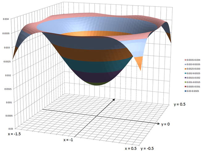
Figure B1.

An upper portion of the toy proton wave function.

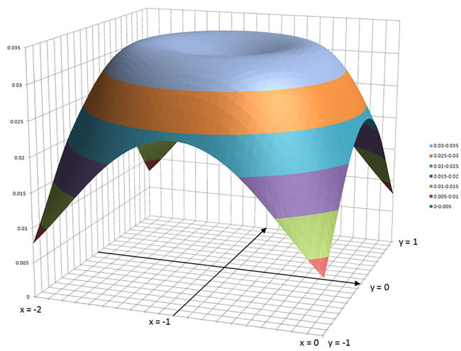
Figure B2.

A middle portion of the toy proton wave function.

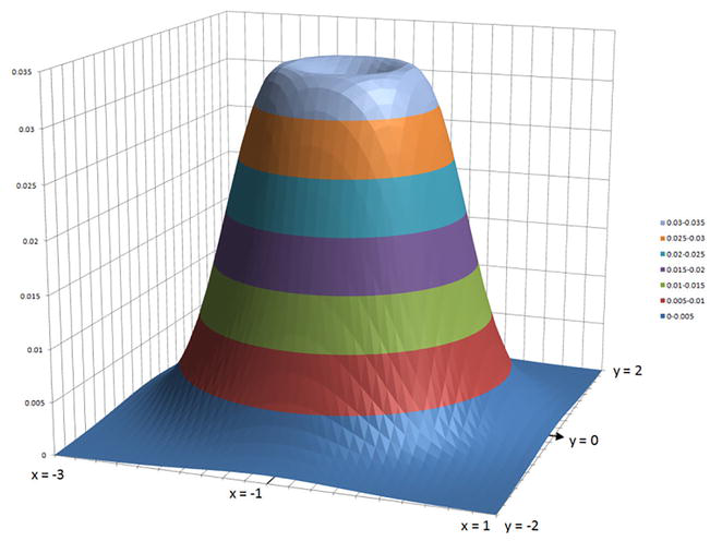
Figure B3.

The entire graph of the toy proton wave function.

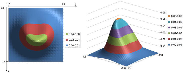
Figure B4.

On realistic ‘sunken proton’ wave function.

References

- 1.
Breidenbach M et al. Observed behavior of highly inelastic electron-proton scattering. Physical Review Letters. 1969; 23 :935-939 - 2.
Levichev AV. Towards a matrix multi-level model of quark-gluon media. JPRM [Internet]. 2016; 10 (2):1493-1496. Available from:http://scitecresearch.com/journals/index.php/jprm/article/view/974 - 3.
Levichev AV. One possible application of the chronometric theory of I.E. Segal: A toy model of quarks and gluons. Journal of Physics: Conference Series. 2019; 1194 :012071 - 4.
Segal IE. Is the cygnet the quintessential baryon? Proceedings of the National Academy of Sciences. 1991; 88 :994-998 - 5.
Wigner EP. On unitary representations of the inhomogeneous Lorentz group. Annals of Mathematics. 1939; 40 (2):149-204 - 6.
Levichev AV, Palyanov AY. On colors and electric charges of quarks: Modeling in terms of groups U(n) and SU(n,n). Mathematical Structures and Modeling. 2020; 4 (56):31-40, in Russian - 7.
Levichev AV. On key properties of the intertwining operators ornament in the matrix multi-level model of the quark-gluon media. In: Proceedings of the All-Russia Conference with the International Participation “Knowledge-Ontology-Theories” (KONТ-2017); 6–8 October 2017 Novosibirsk. Vol. 2. Novosibirsk: Sobolev Institute of Mathematics of the Siberian Division RAS; 2017. pp. 41-47 - 8.
Kon M, Levichev A. Parallelization analysis of space-time bundles and applications in particle physics. In: Proceedings of the All-Russia Conference with the International Participation “Knowledge-Ontology-Theories” (KONТ-2019); 7–11 October 2019 Novosibirsk. Novosibirsk: Sobolev Institute of Mathematics of the Siberian Division RAS; 2019. pp. 385-392 - 9.
Levichev A, Palyanov A. Standard charges of quarks determination in terms of the multi-level model. In: Proceedings of the All-Russia Conference with the International Participation “Knowledge-Ontology-Theories” (KONТ-2019); 7–11 October 2019 Novosibirsk. Novosibirsk: Sobolev Institute of Mathematics of the Siberian Division RAS; 2019. pp. 222-226 - 10.
Jakobsen HP, Levichev AV, Palyanov AY. The Wigner-Segal method as applied to the problem of quarks’ and leptons’ generations. In: Proceedings of the All-Russia Conference with the International Participation “Knowledge-Ontology-Theories” (KONТ-2021); 8--12 November Novosibirsk. Novosibirsk: Sobolev Institute of Mathematics of the Siberian Division RAS; 2021. pp. 344-352. Available from: http://math.nsc.ru/conference/zont/21/index.htm - 11.
Jakobsen HP, Levichev AV. The representation of SU(2,2) which is interpreted as describing chronometric fermions (proton, neutrino, and electron) in terms of a single composition series. Reports on Mathematical Physics. 2022; 90 (1):103-121 - 12.
Levichev A, Palyanov A. The multi-level model for quarks and leptons as the symbiosis of Segal’s chronometry with the standard model. Preprint. 2022. 19 p. This version not peer-reviewed. Full publication to appear soon. DOI: 10.20944/preprints202202.0280.v1 - 13.
Levichev AV. Pseudo-hermitian realization of the Minkowski world through DLF theory. Physica Scripta. 2011; 83 :1-9. Available from:https://iopscience.iop.org/article/10.1088/0031-8949/83/01/015101 - 14.
Levichev AV. Segal’s chronometry: Its development, application to the physics of particles and their interactions, further perspectives. In: Lavrent’ev M, Samoilov V, editors. Poisk matematicheskih zakonomernostei Mirozdania. Novosibirsk: GEO; 2010. pp. 66-99 in Russian - 15.
Paneitz SM, Segal IE, Vogan DA Jr. Analysis in space-time bundles, IV. Journal of Functional Analysis. 1987; 75 :1-57 - 16.
Moylan P. Harmonic analysis on spannors. Journal of Mathematical Physics. 1995; 36 :2826-2879 - 17.
Jakobsen HP. Intertwining differential operators for Mp(n;R) and SU(n; n). Transactions of the American Mathematical Society. 1978; 246 :311-337 - 18.
Jakobsen HP, Vergne M. Wave and Dirac operators and representations of the conformal group. Journal of Functional Analysis. 1977; 24 :52-106 - 19.
Barut AOA. Return to 1932: Proton, electron and neutrino as true elementary constituents of leptons, hadrons and nuclei. In: Quantum Theory and the Structures of Time and Space. Vol. 4. Munich: Carl Hanser Press; 1981. pp. 152-163 - 20.
Varadarajan V. Geometry of Quantum Theory. New York: Springer; 1985. 412 p - 21.
Faessler M. Weinberg angle and integer electric charges of quarks. arXiv. 2013. 6 p. Available from: https://arxiv.org/abs/1308.5900 - 22.
Levichev AV, Klevtsova Y, Palyanov A, Yu AD. Alexandrov would have been 110, and a contribution to chronometry. Mathematical Structures and Modeling. 2022; 2 (62):66-75 in Russian - 23.
Qiu B, Men Y, Wang J, Hui Z. Dosimetry, efficacy, safety, and cost effectiveness of proton therapy for non-small cell lung cancer. Cancers (Basel). 2021; 13 (18):4545. DOI: 10.3390/cancers13184545. Available from:https://www.ncbi.nlm.nih.gov/pmc/articles/PMC8465697/ - 24.
Fitz, Gerald J, Bishop-Jodoin TM, editors. Dosimetry [Internet]. London, UK: IntechOpen; 2022. DOI: 10.5772/intechopen.98044