Determination of Residual Stress by X-Ray Diffraction with the Cos-Alpha Method and Its Application

Abstract

Today, residual stress determination by X-ray diffraction is a well-known method. While all X-ray stress determinations rely on Braggs law to measure the difference in lattice spacing of differently orientated lattice planes, the traditional sin²psi-2θ method uses different incident angles, and the cos-alpha method uses the complete Debye-Scherrer ring diffracted from the sample surface to acquire signals from differently orientated lattice planes. To calculate the residual stress from a Debye-Scherrer ring, the shift and distortion of the ring compared to a ring of an unstressed sample are plotted over cos-alpha. The slope of that plot indicates the stress on the sample surface. While the principal stress directions mostly shift the ring or change its diameter, the shear stresses distort the ring. Using one measurement direction, a plane stress can be calculated. To calculate stresses with the out-of-plane shear stress components, the opposite direction (${\phi }_0$ = 0°; 180°) is needed additionally. To determine the complete stress, tensor measurements from four directions (${\phi }_0$ = 0°; 90°; 180°; 270°) are necessary. Because of the relatively small dimensions of the equipment and the low radiation exposure caused by the device, the method is highly suitable for measuring not only in the lab but also onsite and within production areas. Since the samples do not need to be moved during the measurement, the sample size and weight are not limited. Examples include bearing rings for cranes or mining tools that can be measured onsite.

1. Introduction

This chapter will give an overview of the cos-alpha method of stress determination. The chapter includes the basic principles, information on the equipment used in the method as well as benefits and limitations, especially compared to other X-ray stress analysis methods. Since the cos-alpha method of stress determination was only recently implemented into a commercially available device, this chapter focuses on the mobile stress analyzer of a Japanese manufacturer. The basic principle, however, will be true for most other implementations of the cos-alpha method into a measurement device. The cos-alpha method usually has good agreement with the expected amount of stress in a specimen and other stress determination methods (see [1, 2, 3, 4, 5]).

1.1 Variables

All variables are listed in Table 1:

${ϵ}_{\alpha }$	Strain in $\alpha$-direction
${\theta }_0$	Diffraction angle of an unstressed specimen
${\eta }_0$	Corresponding angle to ${\theta }_0$
$L$	Distance between detector and specimen surface
$L_m$	Distance between detector and specimen surface calculated from the mean radius of the DSR
$r_{\alpha }$	Radius of the DSR at $\alpha$ angle
$r_0$	Radius of the DSR for an unstressed specimen (the same for all $\alpha$ angles)
$r_m$	Mean radius of the DSR
${\sigma }_x$	Stress in x-direction (specimen coordinate system)
${\sigma }_y$	Stress in y-direction (specimen coordinate system)
${\sigma }_z$	Stress in z-direction (specimen coordinate system)
${\tau }_{\mathit{xy}}$	Shear Stress in xy-direction (specimen coordinate system)
${\tau }_{\mathit{xz}}$	Shear Stress in xz-direction (specimen coordinate system)
${\tau }_{\mathit{yz}}$	Shear Stress in yz-direction (specimen coordinate system)
$I_0$	X-ray intensity coming from the X-ray tube
$I\left(l\right)$	X-ray intensity after traveling through material
$l$	X-ray travel length trough material
$\mu$	Energy-dependent mass attenuation coefficient

Table 1.

Used variables.

2. Principles

The measurement of stress in polycrystalline materials is based on the strain measurement and the lattice distances of several lattice planes. These distances can be measured by X-ray diffraction based on Braggs Law.

2.1 Bragg’s law and Debye-Scherrer ring

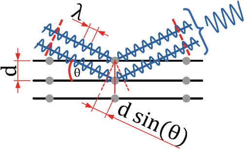
Bragg’s law is a fundamental principle in X-ray crystallography, which explains the behavior of X-rays when they interact with a crystalline material. It was formulated by Sir William Lawrence Bragg and his father, Sir William Henry Bragg, in 1912 [6].

When X-rays encounter a crystal lattice, they are scattered by the atoms within the crystal. Bragg’s law describes the conditions under which constructive interference occurs.

Bragg’s law is mathematically represented as follows:

$$\mathit{n\lambda }=2\mathit{\text{dsinθ}}$$E1

Figure 1 shows the geometric connection of the variables used in Bragg’s law in a crystalline material.

Figure 1.

Bragg’s law.

Since applied and residual stress deform the crystal, the lattice spacing changes, and the Bragg angle changes as well. Using Bragg’s law, the lattice spacing can be calculated with a known X-ray wavelength and a measured diffraction angle.

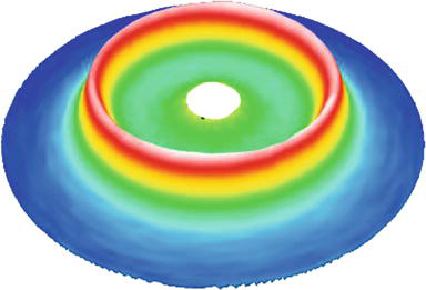
A measurable X-ray peak can be detected from every lattice plane that satisfies Bragg’s law for a given incident angle to the specimen surface. The random orientation of grains in the specimen material leads to a diffraction cone that can be detected as a ring on a two-dimensional detector. This ring is called the Debye-Scherrer Ring (DSR, named after Peter Debye and Paul Scherrer who conducted experiments featuring diffraction rings from powder samples.

Figure 2 shows a three-dimensional depiction of a Debye-Scherrer ring, where height and color indicate the intensity of the signal. A distinct ring can be seen with a moderate half width. For stress-free samples that have enough individual lattice planes contributing to the DSR signal, the ring should be centric to the incident X-ray and have an even distribution of intensity around the circumference.

Figure 2.

Three-dimensional depiction of the DSR data.

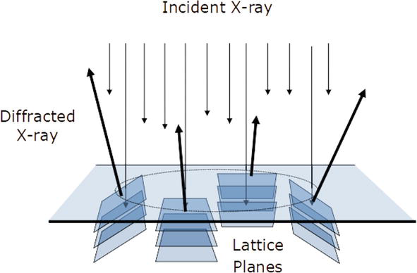
Every single lattice plane acts as a strain gauge in this setup and contributes to the stress calculation. To calculate the strain, and for the stress that has been introduced into the crystal system different, lattice plane orientations have to be considered; and because from a single diffraction peak, the stress and orientation cannot be calculated.

Every lattice orientation to the surface can be described by φ and ψ angles as seen in Figure 3. On the two-dimensional detector, every combination of $\phi$ and $\psi$ angles gives an $\alpha$ angle. The $\alpha$ angle is the azimuthal angle of the detector.

Figure 3.

Different lattice plane orientations that form a diffraction cone.

2.2 Stress determination by cos-alpha method

The cos-alpha method of stress determination has been introduced in Japan in the 1970s by Taira, Tanaka, and Yamasaki [1].

The cos-alpha method uses the complete DSR to get data from different lattice plane orientations instead of using different incident angles.

2.2.1 Deformation and shifting of the Debye-Scherrer ring due to stress

As described in Section 2.1, the azimuthal angle of the detector can be used to describe different lattice plane orientations. When stress is introduced into the specimen, the lattice distances change and give different diffraction angles according to Bragg’s Law. According to the amount and direction of the stress in a given specimen, the DSR will shift and deform according to the strain introduced to the individual lattice planes. Compared to an unstressed specimen such as a powder sample, the ring shift and deformation can be calculated as stress.

Every $\alpha$-angle is linked to a certain $\phi$ and $\psi$ angles representing the angle of the lattice plane to the surface normal and stress direction. Therefore, the effect of stress introduced into the specimen has a different impact on the individual peaks at different $\alpha$.

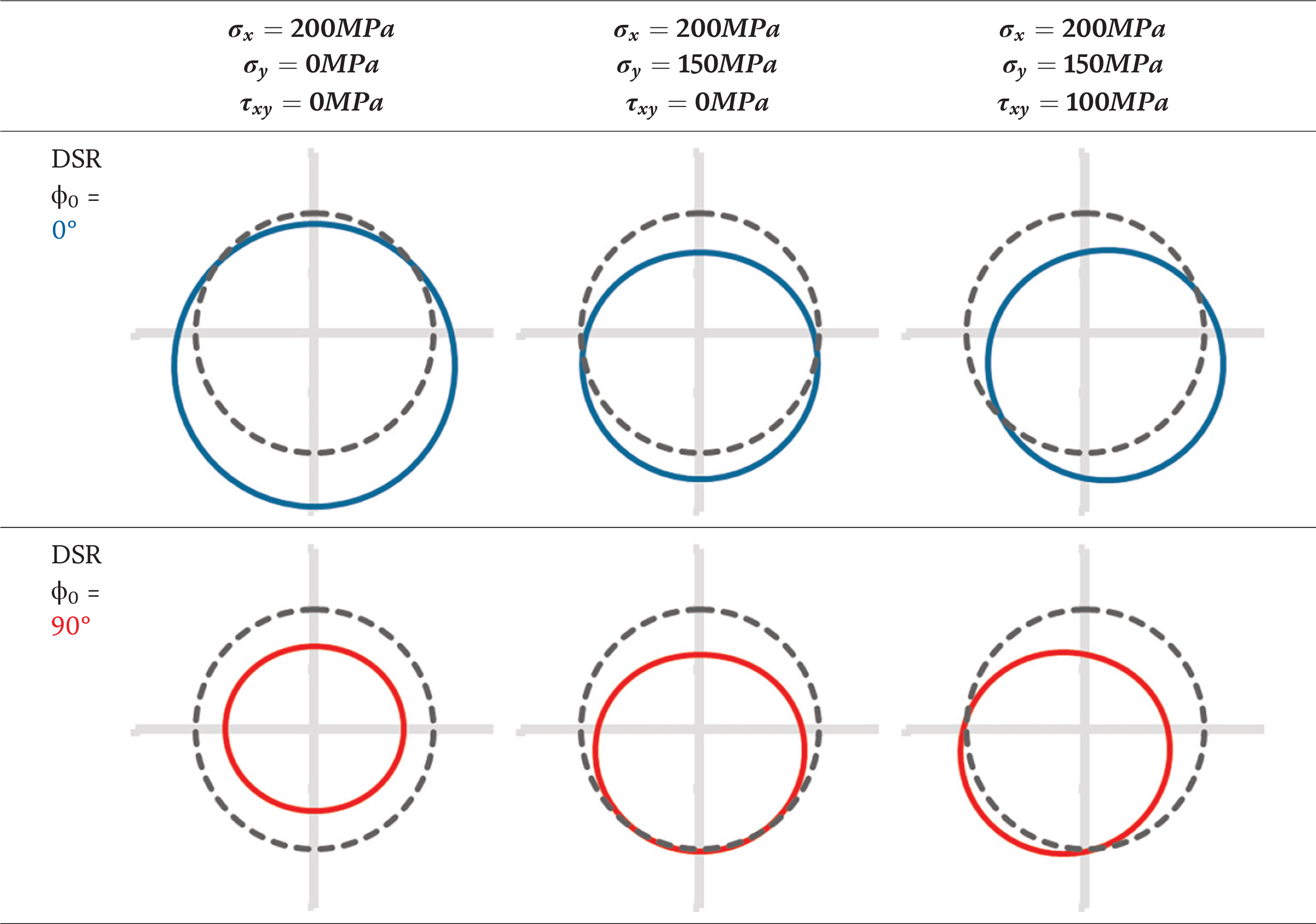
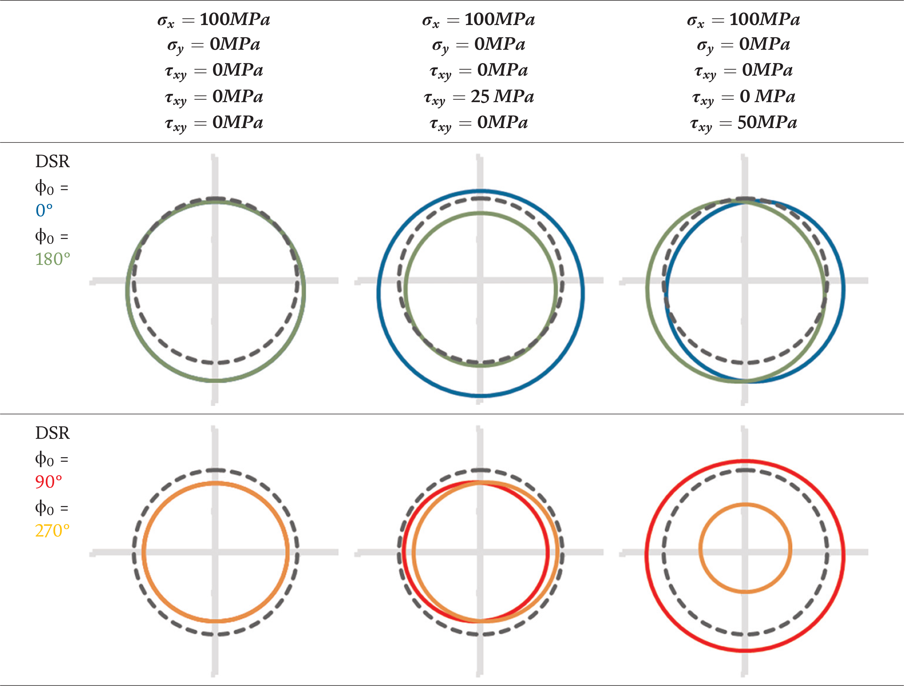
To give a better understanding of the changes in the DSR a plane stress tensor is assumed as follows:

$$\left[\begin{array}{ccc}{\sigma }_x& {\tau }_{\mathit{xy}}& {\tau }_{\mathit{xz}}\\ {\tau }_{\mathit{yx}}& {\sigma }_y& {\tau }_{\mathit{yz}}\\ {\tau }_{\mathit{zx}}& {\tau }_{\mathit{zy}}& {\sigma }_z\end{array}\right]=\left[\begin{array}{ccc}200\mathit{MPa}& 0\mathit{MPa}& 0\mathit{MPa}\\ \dots & 0\mathit{MPa}& 0\mathit{MPa}\\ \dots & \dots & 0\mathit{MPa}\end{array}\right]$$E2

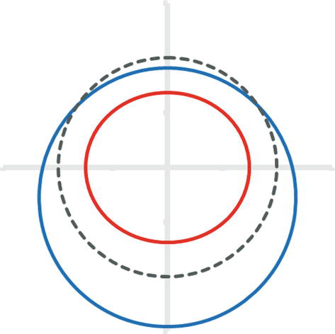
The following figures are created using the stress tensor above. The differences to the unstressed DSR are amplified for better visibility of the changes made to the stressed specimen DSRs.

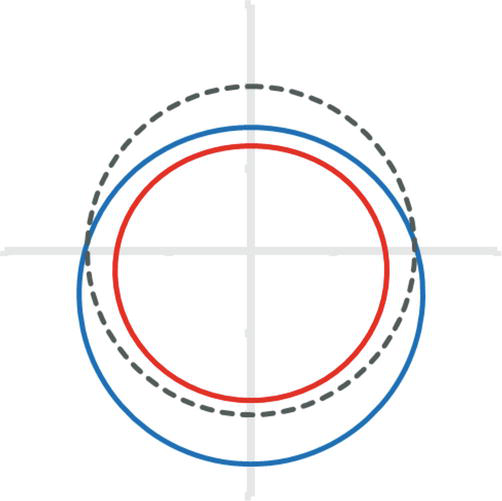
As pictured in Figure 4, the plane stress in the x-direction leads to an enlarged and shifted DSR in the x-direction and a compressed ring in the y-direction.

Figure 4.

DSR for a stressed specimen measured from two directions (${\phi }_0$ = 0° (blue), ${\phi }_0$ = 90° (red) and unstressed specimen (black dashed)).

Introducing 100 MPa of additional stress in the y-direction (${\phi }_0$ = 90°) as well changes the position and size of both rings. While the blue ring (${\phi }_0$ = 0°) is mostly compressed, the red ring (${\phi }_0$ = 90°) is shifted out of the center and is enlarged. The effect is similar to the stress introduction shown above in Figure 4 and can be seen in Figure 5.

Figure 5.

Additional stress from ${\phi }_0$ = 90 (${\phi }_0$ = 0° (blue), ${\phi }_0$ = 90° (red) and unstressed specimen (black dashed)).

The following Table 2 summarizes the influence of the tensor components on the DSR:

Table 2.

Overview of the influence of plane stress on a DSR.

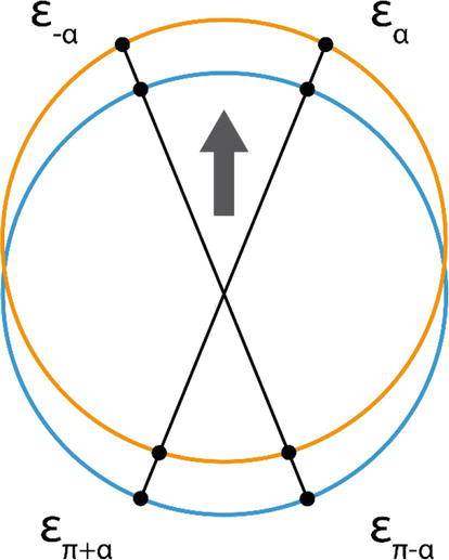
Introducing the out-of-plane shear stress into the material causes the DSR from the opposing direction to shift away from each other. With a plane stress condition, there is no change in the DSR when turning the measurement direction by 180°. The mean value for both rings will be the ring without the out-of-plane shear stress. Where only one DSR is shown, they actually overlap so only one ring is shown (Table 3).

Table 3.

Overview of the influence of out-of-plane shear stress on a DSR.

2.2.2 Determination of stress

The following formula is used to calculate the strain in different $\phi$ and $\psi$ directions from the deformed and shifted Debye-Scherrer ring:

$${ϵ}_{\alpha }=\frac{{\mathit{cos}}^{2}2{\theta }_0}{2\mathit{\text{Ltan}}{\theta }_0}\left(r_{\alpha }-r_{´0}\right).$$E3

To eliminate the necessity to know the distance to the specimen precisely, commercial devices usually use the mean radians computed by the data from the stressed specimen DSR.

From the mean radians, the distance can be calculated as follows:

$$L_m=\frac{r_m}{\mathit{tan}2{\eta }_0}.$$E4

Using $L_m$ instead of $L$ gives you an error of typically less than 0.1%. The strain is then calculated by

$${ϵ}_{\alpha }=\frac{{\mathit{cos}}^{2}2{\theta }_0}{2L_m\mathit{tan}{\theta }_0}\left(r_{\alpha }-r_{´0}\right).$$E5

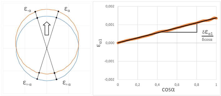
To calculate ${ϵ}_{\alpha 1}$ und ${ϵ}_{\alpha 2},$ four strain directions are used. The four strain values are collected from the same DSR. It gives a relative DSR shift to an unstressed specimen, as seen in Figure 6.

Figure 6.

DSR shift due to stress.

$${ϵ}_{\alpha 1}\equiv \frac{\left({ϵ}_{\alpha }-{ϵ}_{\pi +\alpha }\right)+\left({ϵ}_{-\alpha }-{ϵ}_{\pi -\alpha }\right)}{2}$$E6

This strain is related to stress by the following equation:

$${ϵ}_{\alpha 1}=\frac{-1+\nu }{E}.$$E7

To determine the shear stress components an additional strain parameter is defined:

$${ϵ}_{\alpha 2}\equiv \frac{\left({ϵ}_{\alpha }-{ϵ}_{\pi +\alpha }\right)-\left({ϵ}_{-\alpha }-{ϵ}_{\pi -\alpha }\right)}{2}.$$E8

The strain parameter is connected to the shear stress components as follows:

$${ϵ}_{\alpha 2}=2\frac{1+\nu }{E}.$$E9

To determine stress from Eq. (7), the equation is converted to feature all stress components on one side of the equation and the constants and ring shift on the other side. For measurement volumes that are close to the sample surface, ${\sigma }_z$ can be assumed to be zero.

$${ϵ}_{\alpha 1}=\frac{-1+\nu }{E}$$E10

$$\frac{{\partial ϵ}_{\alpha 1}}{\partial \mathit{\text{cosα}}}=\frac{-1+\nu }{E}$$E11

$${\sigma }_x+2{\tau }_{\mathit{zx}}\frac{\mathit{cos}2{\psi }_0}{\mathit{sin}2{\psi }_0}=\frac{-E}{1+\nu }\frac{1}{\mathit{sin}2\mathit{\text{ηsin}}2{\psi }_0}\frac{\partial {ϵ}_{\alpha 1}}{\partial \mathit{\text{cosα}}}$$E12

The azimuthal angle-dependent relative ring shift $\left(\partial {ϵ}_{\alpha 1}/\partial \mathit{\text{cosα}}\right)$ can be depicted as a plot where the slope represents the stress in the specimen, as shown in Figure 7 below.

Figure 7.

Cos-alpha plot.

To determine ${\sigma }_x,$ an additional measurement direction ${\phi }_0$ is necessary to cancel out ${\tau }_{\mathit{zx}}$. Because the shear stress changes sign when measured from the opposed direction, one way to cancel out ${\tau }_{\mathit{zx}}$ is measuring from ${\phi }_0=0°$ and ${\phi }_0=180°$ and calculating the average as follows:

$${\sigma }_x=\frac{\left[\left({\sigma }_{x,{\phi }_0=0°},+,2,{\tau }_{\mathit{zx},{\phi }_0=0°},\frac{\mathit{cos}2{\psi }_0}{\mathit{sin}2{\psi }_0}\right),+,\left({\sigma }_{x,{\phi }_0=180°},+,2,{\tau }_{\mathit{zx},{\phi }_0=180°},\frac{\mathit{cos}2{\psi }_0}{\mathit{sin}2{\psi }_0}\right)\right]}{2}$$E13

$$2{\tau }_{\mathit{zx},{\phi }_0=0°}\frac{\mathit{cos}2{\psi }_0}{\mathit{sin}2{\psi }_0}=-2{\tau }_{\mathit{zx},{\phi }_0=180°}\frac{\mathit{cos}2{\psi }_0}{\mathit{sin}2{\psi }_0}$$E14

$${\sigma }_x=\frac{{\sigma }_{x,{\phi }_0=0°}+{\sigma }_{x,{\phi }_0=180°}}{2}$$E15

$${\sigma }_x=\frac{-E}{1+\nu }\frac{1}{\mathit{sin}2\mathit{\text{ηsin}}2{\psi }_0}\frac{\frac{\partial {ϵ}_{\alpha 1,{\phi }_0=0°}}{\partial \mathit{\text{cosα}}}+\frac{\partial {ϵ}_{\alpha 1,,{\phi }_0=180°}}{\partial \mathit{\text{cosα}}}}{2}$$E16

A similar equation can be used to determine ${\sigma }_y$.

$${\sigma }_y=\frac{\left[\left({\sigma }_{y,{\phi }_0=90°},+,2,{\tau }_{\mathit{zy},{\phi }_0=90°},\frac{\mathit{cos}2{\psi }_0}{\mathit{sin}2{\psi }_0}\right),+,\left({\sigma }_{y,{\phi }_0=270°},+,2,{\tau }_{\mathit{zy},{\phi }_0=270°},\frac{\mathit{cos}2{\psi }_0}{\mathit{sin}2{\psi }_0}\right)\right]}{2}$$E17

$$2{\tau }_{\mathit{zy},{\phi }_0=90°}\frac{\mathit{cos}2{\psi }_0}{\mathit{sin}2{\psi }_0}=-2{\tau }_{\mathit{zy},{\phi }_0=270°}\frac{\mathit{cos}2{\psi }_0}{\mathit{sin}2{\psi }_0}$$E18

$${\sigma }_y=\frac{{\sigma }_{y,{\phi }_0=90°}+{\sigma }_{y,{\phi }_0=270°}}{2}$$E19

$${\sigma }_y=\frac{-E}{1+\nu }\frac{1}{\mathit{sin}2\mathit{\text{ηsin}}2{\psi }_0}\frac{\frac{\partial {ϵ}_{\alpha 1,{\phi }_0=90°}}{\partial \mathit{\text{cosα}}}+\frac{\partial {ϵ}_{\alpha 1,,{\phi }_0=270°}}{\partial \mathit{\text{cosα}}}}{2}$$E20

To calculate the shear stress the equation from above is used.

$${ϵ}_{\alpha 2}=2\frac{1+\nu }{E}$$E21

$$\frac{{\partial ϵ}_{\alpha 2}}{\partial \mathit{\text{sinα}}}=2\frac{1+\nu }{E}$$E22

$${\tau }_{\mathit{xy}}+{\tau }_{\mathit{yz}}\frac{\mathit{cos}{\psi }_0}{\mathit{sin}{\psi }_0}=\frac{{\partial ϵ}_{\alpha 2}}{\partial \mathit{\text{sinα}}}\frac{E}{2\left(1+\nu \right)}\frac{1}{\mathit{sin}2\mathit{\text{ηsin}}{\psi }_0}$$E23

Similar to the determination of ${\sigma }_x$, an opposing measurement direction is needed to cancel out the out-of-plane shear stress component.

$${\tau }_{\mathit{xy},{\phi }_0=0°,180°}=\frac{\left({\tau }_{\mathit{xy},{\phi }_0=0°}+{\tau }_{\mathit{yz},{\phi }_0=0°}\frac{\mathit{cos}{\psi }_0}{\mathit{sin}{\psi }_0}\right)+\left({\tau }_{\mathit{xy},{\phi }_0=180°}+{\tau }_{\mathit{yz},{\phi }_0=180°}\frac{\mathit{cos}{\psi }_0}{\mathit{sin}{\psi }_0}\right)}{2}$$E24

$${\tau }_{\mathit{yz},{\phi }_0=0°}\frac{\mathit{cos}{\psi }_0}{\mathit{sin}{\psi }_0}=-{\tau }_{\mathit{yz},{\phi }_0=180°}\frac{\mathit{cos}{\psi }_0}{\mathit{sin}{\psi }_0}$$E25

$${\tau }_{\mathit{xy},{\phi }_0=0°,180°}=\frac{{\tau }_{\mathit{xy},{\phi }_0=0°}+{\tau }_{\mathit{xy},{\phi }_0=180°}}{2}$$E26

$$\frac{{\tau }_{\mathit{xy},{\phi }_0=0°}+{\tau }_{\mathit{xy},{\phi }_0=180°}}{2}=\frac{E}{2\left(1+\nu \right)}\frac{1}{\mathit{sin}2\mathit{\text{ηsin}}{\psi }_0}\frac{\left(\frac{\partial {ϵ}_{\alpha 2,{\phi }_0=0°}}{\partial \mathit{\text{sinα}}}+\frac{\partial {ϵ}_{\alpha 2,{\phi }_0=180°}}{\partial \mathit{\text{sinα}}}\right)}{2}$$E27

The same derivation can be made for the other two stress directions.

$${\tau }_{\mathit{xy},{\phi }_0=90°,270°}=\frac{\left({\tau }_{\mathit{xy},{\phi }_0=90°}+{\tau }_{\mathit{yz},{\phi }_0=90°}\frac{\mathit{cos}{\psi }_0}{\mathit{sin}{\psi }_0}\right)+\left({\tau }_{\mathit{xy},{\phi }_0=270°}+{\tau }_{\mathit{yz},{\phi }_0=270°}\frac{\mathit{cos}{\psi }_0}{\mathit{sin}{\psi }_0}\right)}{2}$$E28

$${\tau }_{\mathit{yz},{\phi }_0=90°}\frac{\mathit{cos}{\psi }_0}{\mathit{sin}{\psi }_0}=-{\tau }_{\mathit{yz},{\phi }_0=270°}\frac{\mathit{cos}{\psi }_0}{\mathit{sin}{\psi }_0}$$E29

$${\tau }_{\mathit{xy},{\phi }_0=90°,270°}=\frac{{\tau }_{\mathit{xy},{\phi }_0=90°}+{\tau }_{\mathit{xy},{\phi }_0=270°}}{2}$$E30

$$\frac{{\tau }_{\mathit{xy},{\phi }_0=90°}+{\tau }_{\mathit{xy},{\phi }_0=270°}}{2}=\frac{E}{2\left(1+\nu \right)}\frac{1}{\mathit{sin}2\mathit{\text{ηsin}}{\psi }_0}\frac{\left(\frac{\partial {ϵ}_{\alpha 2,{\phi }_0=90°}}{\partial \mathit{\text{sinα}}}+\frac{\partial {ϵ}_{\alpha 2,{\phi }_0=270°}}{\partial \mathit{\text{sinα}}}\right)}{2}$$E31

From all four stress directions, a more accurate shear stress can be calculated.

$${\tau }_{\mathit{xy}}=\frac{{\tau }_{\mathit{xy},{\phi }_0=0°,180°}+{\tau }_{\mathit{xy},{\phi }_0=90°,270°}}{2}$$E32

$${\tau }_{\mathit{xy}}=\frac{E}{2\left(1+\nu \right)}\frac{1}{\mathit{sin}2\mathit{\text{ηsin}}{\psi }_0}\left(\frac{\frac{\left(\frac{\partial {ϵ}_{\alpha 2,{\phi }_0=0°}}{\partial \mathit{\text{sinα}}}+\frac{\partial {ϵ}_{\alpha 2,{\phi }_0=180°}}{\partial \mathit{\text{sinα}}}\right)}{2}+\frac{\left(\frac{\partial {ϵ}_{\alpha 2,{\phi }_0=90°}}{\partial \mathit{\text{sinα}}}+\frac{\partial {ϵ}_{\alpha 2,{\phi }_0=270°}}{\partial \mathit{\text{sinα}}}\right)}{2}}{2}\right)$$E33

$${\tau }_{\mathit{xy}}=\frac{E}{2\left(1+\nu \right)}\frac{1}{\mathit{sin}2\mathit{\text{ηsin}}{\psi }_0}\left(\frac{\frac{\partial {ϵ}_{\alpha 2,{\phi }_0=0°}}{\partial \mathit{\text{sinα}}}+\frac{\partial {ϵ}_{\alpha 2,{\phi }_0=180°}}{\partial \mathit{\text{sinα}}}+\frac{\partial {ϵ}_{\alpha 2,{\phi }_0=90°}}{\partial \mathit{\text{sinα}}}+\frac{\partial {ϵ}_{\alpha 2,{\phi }_0=270°}}{\partial \mathit{\text{sinα}}}}{4}\right)$$E34

To determine the out-of-plane shear stress the following equation can be used:

$${\tau }_{\mathit{yz}}=\frac{E}{2\left(1+\nu \right)}\frac{1}{\mathit{sin}2\mathit{\text{ηsin}}{\psi }_0}\frac{\left(\frac{\partial {ϵ}_{\alpha 2,{\phi }_0=0°}}{\partial \mathit{\text{sinα}}}-\frac{\partial {ϵ}_{\alpha 2,{\phi }_0=180°}}{\partial \mathit{\text{sinα}}}\right)\mathit{tan}{\psi }_0}{2}$$E35

For plane stress condition, only one measurement per stress direction is needed. Under the assumption of a plane stress state, the following equation can be established:

$${\sigma }_z={\tau }_{\mathit{zx}}={\tau }_{\mathit{zy}}=0$$E36

$${\sigma }_x+2{\tau }_{\mathit{zx}}\frac{\mathit{cos}2{\psi }_0}{\mathit{sin}2{\psi }_0}=\frac{-E}{1+\nu }\frac{1}{\mathit{sin}2\mathit{\text{ηsin}}2{\psi }_0}\frac{\partial {ϵ}_{\alpha 1}}{\partial \mathit{\text{cosα}}}$$E37

$${\sigma }_x=\frac{-E}{1+\nu }\frac{1}{\mathit{sin}2\mathit{\text{ηsin}}2{\psi }_0}\frac{\partial {ϵ}_{\alpha 1}}{\partial \mathit{\text{cosα}}}$$E38

For further information about the equations featured in this section, please refer to [7, 8].

2.3 Depth of penetration

Similar to other X-ray diffraction techniques, the penetration depth of the measurement is dependent on the wavelength; therefore, X-ray energy and the specimen material respond to the radiation.

The following equation gives the X-ray intensity after a certain travel length through a given material [6]:

$$I\left(l\right)=I_0{e}^{-\mathit{\mu l}}$$E39

Penetration depth is defined as the travel length through a material where

$$\frac{I\left(l\right)}{I_0}=\frac{1}{e}$$E40

To calculate the penetration depth, the equation can be solved by $l$

$$\mathit{ln}\frac{1}{e}=-\mathit{\mu l}$$E41

$$l=\frac{1}{\mu }$$E42

This is true for X-rays that enter and leave the specimen perpendicular to the surface.

The following table gives penetration depths for different specimen materials at different angles:

As shown in Table 4, the penetration depth used in X-ray stress analysis is quite shallow, and creating a stress depth profile requires removal of surface material to access deeper layers. The challenges and procedure to do so can be found in Section 3.7.

Fe (${\psi }_0=35°$)Cr-Kα Radiation	4,6 μm
Al (${\psi }_0=30°$)Cr-Kα Radiation	10,3 μm
Ni (${\psi }_0=35°$)Cr-Kα Radiation	3,2 μm
Fe (${\psi }_0=30°$)Cr-Kβ Radiation	6,3 μm

Table 4.

Penetration depths for different material pairs.

3. Apparatus

3.1 Diffraction geometry

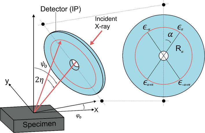
The cos-alpha method uses a fixed angle to the two-dimensional detector; therefore, the devices built using this method are usually mechanically simpler than conventional devices.

As shown in Figure 8, the incident X-ray goes through the detector and meets the sample surface at an angle ${\psi }_0.$ At the lattice planes of the measurement volume, diffraction occurs, and the diffracted beams travel back to the detector under an angle of $2\theta$. The corresponding angle $2\eta$ is the opening angle of the diffraction cone. The rotational angle around the z-axis of the sample coordinate system ${\phi }_0$ marks the measurement direction as well.

Figure 8.

Diffraction geometry of the cos-alpha method.

Because the diffraction angle $2\theta$ is a specimen material, and the X-ray tube depended to different detector distances are necessary to collect the complete DSR data. The measurement, however, is independent from the specimen distance because the mean radians of the DSR can be used instead, as described in Eq. (4).

3.2 Multi-exposure technique

Triaxial stress states require the operator to perform additional measurements from additional incident directions ${\phi }_0$. While a single incident direction is sufficient for plane stress conditions, the presence of the out-of-plane shear stress requires for one measurement direction at least two measurements and tensor at least three, or better, four directions for the complete stress tensor. To gather the additional data, the alignment of the tube-detector unit and specimen surface can be changed by either turning or tilting one of both.

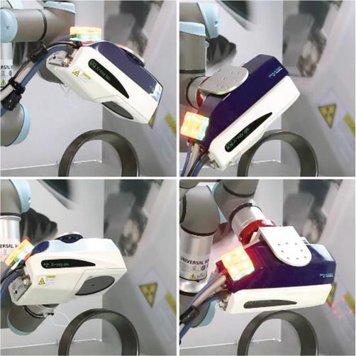
Figure 9 shows a possible setup to collect the data necessary to calculate the complete stress tensor. Instead of turning the device or specimen, the device is tilted in four different directions. In the calculation, the orientation of the detector has to be considered. This method is suitable for automated measurements of medium-sized specimens. The back of the device will collide with the big enough specimen in the ${\phi }_0=180°$ configuration. Another configuration is needed for this kind of specimen.

Figure 9.

One possible tube-detector unit to specimen alignment for stress tensor calculation.

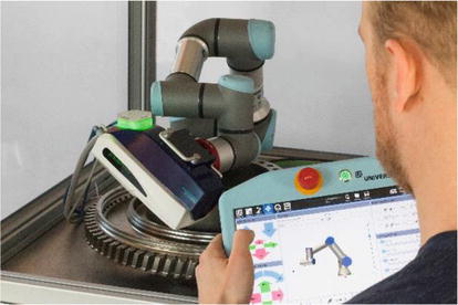
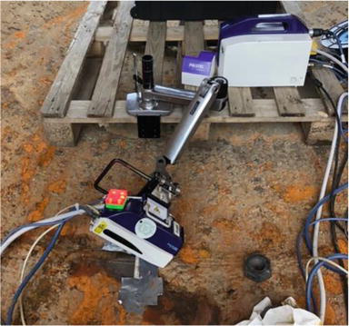
Since the tilting and turning of the tube-detector unit to the specimen needs to be repeated for all measurement positions, using automated positioning can save valuable time. The use of a six-axis robot, the position of the device relative to the surface is shown in Figure 10.

Figure 10.

Setup of an automated stress determination.

3.3 Major components of cos-alpha diffractometers

3.3.1 X-ray tube

The X-ray tubes used in cos-alpha diffractometers are similar to the ones used in sin²psi devices. However, because the complete DSR is used, cos-alpha devices usually feature X-ray tubes that use less electrical power to operate. This leads to tube designs that can be air-cooled and improvements in the portability of the whole system.

3.3.2 Optics

Collimators are used to focus the X-ray beam onto the surface. Since the X-ray will usually go through the detector when applying the cos-alpha technique, the collimators are often installed into the detector. This gives the benefit of an easy alignment of the X-ray to the detector. In this way, the detector will always be perpendicular to the incident X-ray. While other shapes other than round collimators are theoretically possible, they are not common because the movement of the tube-detector unit is usually easier than a collimator change. In addition, the detector is often read out while spinning so that uneven weight distributions should be avoided.

3.3.3 Detector

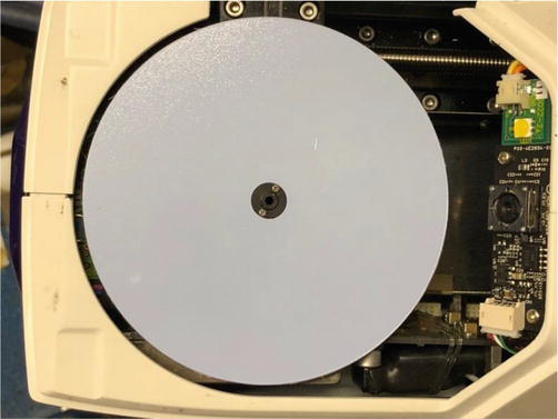
In the past, the only possibility to analyze a DSR was to expose the diffraction cone on a photo-optical material [9]. About 40 years ago, the first steps were taken to develop the so-called MAD detectors that are sensitive to X-rays with low energy. The X-ray intensities are stored in the detector by lifting electrons to metastable positions. The electrons will drop to their original energy level when exposed to a normal He-Ne laser. The now-radiated energy is detected by a scintillation counter. The local resolution of the detector is only determined by the spot size of the laser. In the last 20 years, huge detectors have been developed for medical applications. An implementation of a stress analyzer of this detector technique was a detector that needed to be removed from the measurement device to be read out in a separate machine. Modern implementations of MAD detectors in cos-alpha devices include the read-out mechanism into the tube-detector unit. Figure 11 shows the detector on an X-ray diffractometer. The diameter of the detector is about 10 cm. The detector is read out with the He-Ne-Laser spirally such as the track of a record. The spiral pitch of the laser beam path has a distance of 20–100 μm. The read-out time is dependent on the spiral pitch, but it is faster than 20 s. This type of detector has a long lifetime. For a more detailed description of the detector in relation to the Debye-Scherrer ring, please refer to [10].

Figure 11.

A MAD-detector for detecting a complete DSR.

3.4 Sample positioning

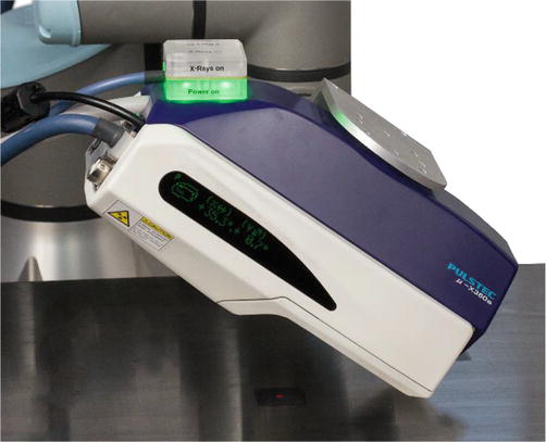
This section focuses on the sample positioning with the X-ray stress analyzer μ-X360s manufactured by Pulstec in Japan. Other cos-alpha devices might feature similar position guidance, but the application of this chapter’s description needs to be checked.

To help set up the irradiation area, a LED is used that is guided through the collimator and meets the sample surface at the same position as the radiation would do. The equipment features an integrated digital angle gauge to adjust the incident angle and a camera to roughly determine the measurement distance by triangulation. The angle gauge shows two values, one for the tilting in measurement direction and the other for the perpendicular direction. Both are in relation to Earth’s gravitational field but can be adjusted to differ in case the specimen surface normal is not parallel to the gravitational field. Checking the incident angle with a ruler helps to verify the measurement setup. Figure 12 shows a setup of a stress measurement on an induction hardened part.

Figure 12.

Measurement guidance systems of the μ-X360s.

The measurement results are not sensitive to wrong angle setups as shown in [11]. An incorrect angle setup has a bigger impact on the calculated shear stresses than on the normal stress directions (see also Section 3.7 for the measurement procedure).

3.5 Radiation and material selection

Different specimen materials require different radiation energies; therefore, wavelengths have to match the distances of the atomic layers. This cannot be achieved by using only one anode material. Table 5 shows the various possibilities between the anode material and specimen material. If there are multiple anode options for the same specimen material, especially in alloys, the option with the smallest number of rings should be chosen to obtain a clear, reliable reflected signal. Kα should be chosen over K_β because the X-ray intensity will be higher.

Anode Material	Characteristic Wavelength used	Specimen Material	Lattice plane	Bragg Angle
Cr	Kα	Ferritic Steel	211	156,396°
	Kα	Aluminum Alloy	222	157,041°
	Kα	Aluminum Alloy	311	139,528°
	Kα	Nickel (pure)	311	158,330°
	Kβ	Nickel Alloy	311	150,876°
	Kβ	Austenitic Steel	311	148,513°
	Kα	Cobalt-Chromium Alloy	110	131,363°
	Kα	Neodynium	211	144,336°
	Kα	Zirconium	133	152,339°
Cu	Kα	Copper Alloy	420	144,982°
	Kα	Copper Alloy	311	136,721°
	Kα	Nickel (pure)	420	156,705°
	Kα	Nickel Alloy	420	156,749°
Co	Kα	Ferritic Steel	301	161,861°
	Kα	Aluminum Alloy	331	148,992°
	Kα	Aluminum Alloy	420	162,715°
	Kα	Chromium	310	157,000°
	Kα	Magnesium Alloy	204	140,728°
	Kα	Magnesium Alloy	300	150,095°
Mn	Kα	Austenitic Steel	311	152,295°
	Kα	Copper	311	149,479°
	Kα	Nickel (pure)	311	164,424°
	Kα	Nickel Alloy	311	155,321°
	Kα	Cobalt-Chromium Alloy	112	157,598°
V	Kα	Titanium Alpha Alloy	103	140,077°
	Kα	Tungsten	211	151,552°
	Kα	Tungsten-Carbide	111	152,053°
	Kα	Copper	220	156,972°
	Kα	Silicon Carbide	411	152,891°
	Kβ	Ferritic Steel	211	154,867°
	Kα	Austenitic Steel	220	160,906°

Table 5.

X-ray tube anode material vs. specimen material.

3.6 Sample issues

The explanations in Section 3.6 are mostly applicable to the sin²psi-2θ method because both methods use a part (sin²psi-2θ) or the full DSR (cos-alpha) and therefore face similar restrictions.

3.6.1 Sample preparation

For accurate and repeatable results, the specimen should have a fixed position relative to the tube-detector unit during irradiation. Changes in the positioning, even small ones such as vibrations, should be prevented by fixating the specimen. A coordinate system that is drawn on the specimen helps identify the measurement position and the orientation even after the measurement has finished.

If the sample has a clean surface without any coating or leftover contamination from previous processes, the measurement can be started directly. However, if there is, for instance, scale or rust present on the surface, a measurement is mostly impossible. The penetration depth of X-rays is less than 10 μm, as described in Section 2.3. Therefore, to measure the sample accurately, any coating must be removed by chemical treatment. This can be done through electropolishing or similar methods. It is crucial to avoid mechanical methods of removal because every mechanical treatment such as grinding drastically changes the residual stress state. In approximately 300-μm depth, the influence of the mechanical surface treatment has mostly disappeared.

3.6.2 Textured grain structure and coarse grain

All X-ray diffraction stress analysis methods assume an isotropic material behavior when applying Hook’s law to convert the measured strains to stress values. This, however, is only true if the lattice planes occur randomly in the specimen material. A texture, meaning a nonrandom distribution of lattice plane orientations in the material leads to anisotropic material behavior, and therefore to errors in the calculation of stress. The texture can, however, be spotted when intensities of differently orientated diffraction cones are compared. With a fully random orientation, the lattice plane orientation should not have an influence on the intensity heights.

Texture will occur, for example, in cold-drawn pipes, where the drawing process leads to the preferred orientation of the lattice planes.

Another reason for the uneven intensity distributions is coarse grain leading to not enough lattice planes to contribute to a complete DSR. While the intensity differences can be observed in all X-ray diffraction stress analysis methods, the cos-alpha method has the benefit that the data from the complete DSR give a more complete picture in the same measurement time.

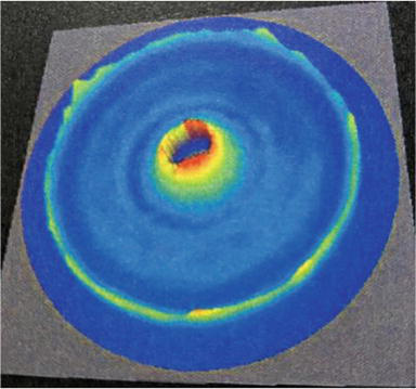
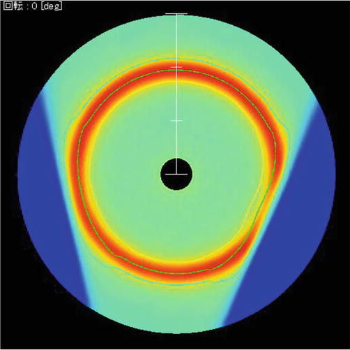
Figure 13 displays the intensity distribution of a cold-drawn pipe that is coarse-grained and textured at the same time. The incompleteness of the ring increases as the radiated spot gets smaller [7, 12] In this particular case, the difference between the maximum and minimum intensities has a ratio of ρ = 3.4; whereas for the iron powder, it is less than ρ = 1.5. The diameter of the X-ray spot utilized is 4 mm.

Figure 13.

DSR of a cold drawn pipe.

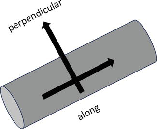
3.6.3 Curved samples

The behavior of the results obtained from curved surfaces is similar to that of the sin²psi-2θ method. This technique can be used in two ways: measuring along the curvature and measuring perpendicular to it, as shown in Figure 14.

Figure 14.

Definition of the directions.

As described in Section 2.1, every section of the DSR is linked to another combination of $\psi$ and $\phi$ angles of the lattice planes. The different orientations are needed to calculate the stress amount and direction. When measuring on a curved sample, the lattice plane orientation to the surface normal is not uniform anymore, and there is no way to determine it from the DSR afterward. Because the $\alpha$-angles cannot precisely be linked to the lattice plane orientation an, error is added to the stress values. If the measurement is not performed on the top of the curvature, there is an additional error.

Because the measurement is performed under an incident angle of close to 30°, the measurement spot is distorted alongside the measurement direction. This leads to a higher sensitivity to curvature when measuring perpendicular compared to a measurement alongside.

According to [13], the first results indicate that for accurate measurements along the curvature, the X-ray spot diameter should be no more than 20% of the curvature diameter and no more than 10% in the perpendicular direction. However, recent studies by [14] suggest that more than 20% in the direction parallel to the surface can also be reliable.

3.6.4 Huge components

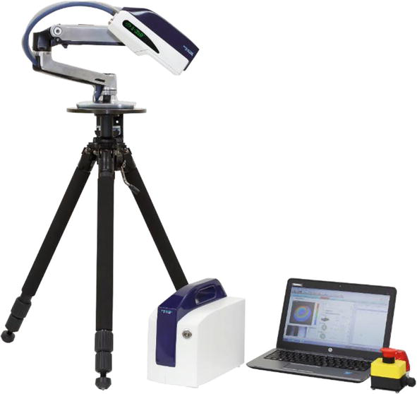
To preserve the overall stress in a specimen or to save it for future testing, it is often times necessary to perform measurements without cutting a smaller piece out of big components. This usually is also very time-consuming and requires a lot of experience to not introduce additional residual stress. Some specimens are also too big to be moved or would fail during the shipment. For these reasons, measurements are often easier carried out onsite and without cutting. This creates the need for portable X-ray stress analyzers, which should be lightweight, uncomplicated to set up and have small dimensions for good accessibility. Cos-alpha stress analyzers usually fulfill the above-mentioned requirements (see Figure 15). The following examples illustrate this point.

Figure 15.

X-ray stress analyzer mounted on a tripod for mobile use.

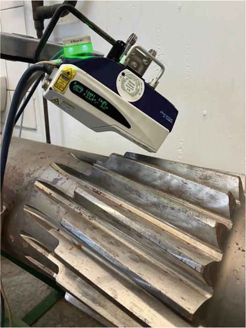
The first example is a mining equipment’s driving shaft that has been measured at the company’s production site. Because residual stress alongside the tooth is a crucial factor in determining durability, a stress profile alongside the tooth was measured. The surface measurements required no additional sample preparation and are shown in Figure 16.

Figure 16.

Setup to measure a driving shaft (mining equipment).

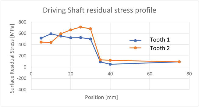
The tooth had a different treatment in the first 35 mm of the measurement track, as can be seen in Figure 17. There was a slight difference when two tooths were compared to one another, but the additional treatment can be seen quite well.

Figure 17.

Residual stress depth profile parallel to the tooth.

Please note that in the above example, the measurement was done without removing any components from the mining equipment in the lab. This onsite measurement technique clearly highlights the advantages of using a small-sized X-ray diffractometer.

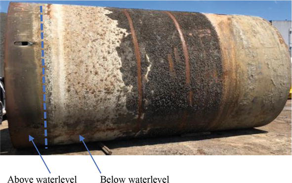
The second example is a monopile, which is a tube with a diameter of 3 m, that is rammed into the ground underwater. The other end of the tube protrudes from the water and has a wind turbine mounted onto it for an offshore wind park. Figure 18 shows the section of the monopile that is under the water and the portion that is outside of it. The goal was to determine the residual stresses of the welding seam after being submerged for more than 20 years. The measuring station can be seen in Figure 19.

Figure 18.

Upper part of a monopile.

Figure 19.

Setup of the X-ray diffractometer inside the monopile for a stress measurement at the welding seam.

It is worth noting that by conducting an onsite residual stress measurement, it is possible to obtain important information about the condition and stability of such large structures.

More examples of these big components can be seen in [15].

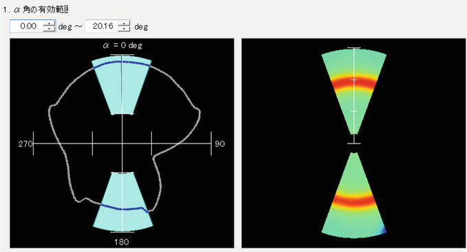
3.6.5 Obstructions

The parts with complex geometries or even undercuts are a challenging measurement task because they will block part of the DSR needed for the stress calculation. While a more complete DSR will lead to better results, it is possible to use only a part of the DSR for the stress calculation. Because every position of the cos-alpha plot consists of four strain values (see Eq. [6]), data get excluded crosswise.

A typical example is a gear tooth root where information of the DSR gets cut off by the tooth flanks (Figure 20).

Figure 20.

DSR of gear tooth root with obstructions on both sides.

Because not only the peak position of the DSR is missing but also the background radiation, there are usually problems with the peak determination even if the DSR peak is not obstructed. Displaying the peak position on an enlarged scale helps to identify the areas that should be excluded in the measurement and shows such as an enlarged DSR with the highlighted area from which the information is used in the stress calculation (Figure 21).

Figure 21.

Cutoff areas of the DSR that are distorted by the obstruction.

3.6.6 Surface roughness

Surface roughness can significantly affect the results of residual stress measurements. The incident angle of the X-ray, in combination with roughness, is an important factor to consider. For instance, there are surfaces that have been shot peened without any notable roughness [16]. If the roughness is Rz = 25 μm, the difference in results between measuring at an incident angle of 15° (measured perpendicular to the surface) and an angle of 45° is 25%. When the angle is high, only the surface peaks are measured, which can relax because they have no support from the material around them, leading to lower residual stress measurement values.

In line with the PV1005 guideline provided by Volkswagen [17], the surface should be electrolytically smoothed to a maximum of 5 μm to obtain more reliable results. This underscores the importance of considering surface roughness in carrying out residual stress measurements, particularly for precise results.

3.7 Residual stress depth profiling

Because of the limited penetration depth of X-rays, usually less than 10 μm, material removal is necessary to measure residual stress at greater depths. However, it is crucial to ensure that the removal process does not alter the residual stress state. Mechanical removal methods can indeed change the residual stress state, making chemical removal the preferred option.

To prevent significant changes in the residual stress state, a masking technique can be employed during chemical removal. Applying a mask with an 8-mm diameter hole is a good choice because it balances the influence on residual stresses with the goal of obtaining a flat surface. The different electrical field effects at the edges of the hole can cause either increased removal or a rounded shape, depending on the specific chemical used. It is important to note that the surface in the area of the removal site may become curved.

Chemical removal, also known as electropolishing, can be achieved using mild acids such as NH4Cl, as well as other similar acids and salts [18]. However, it is advisable to avoid removing large areas, as this can significantly alter the residual stress state and require subsequent correction [19, 20]. Careful consideration of the chemical removal process is essential to maintain the integrity of residual stress measurements.

3.8 Residual stress mapping

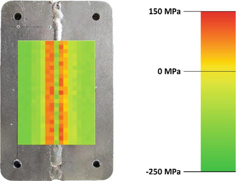
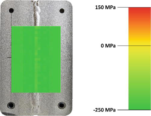
Because residual stresses influence material behavior such as fatigue life quite drastically, a stress mapping can be very helpful if no obvious weak point has a stress concentration. While stress mappings can be carried out manually for bigger measurement volumes, an automated approach is more suitable. With the use of a linear stage or a robot, even big mappings can be carried out with a reasonable amount of setup time. In addition to the automation needed to perform big stress mappings, a stress analyzer used for this task should be insensitive to misalignments in distances and incident angle, have a short measurement time, and should be compact so the specimen geometries allow for a complete scan of the surface. Because cos-alpha devices usually fulfill the aforementioned properties, they are particularly suitable for this kind of measurement task. The following example is a welded part that has been measured before and after a shot peening treatment (Figure 22).

Figure 22.

Specimen before shot peening with distinct welding stress.

The difference in stress can be easily seen from the heat map of the measured stresses. Before the shot peening tensile stresses can be found in the heat-influenced zone, only compressive stresses are left at the surface afterward. A part treated such as this is usually going to have a substantially longer fatigue life (Figure 23).

Figure 23.

Specimen after shot peening with uniform compressive stress.

For more information on optimizing production processes with residual stress measurements, please refer to [21].

3.9 Measurement procedure

This section focuses on the Pulstec μ-X360s, which is currently the only commercially available diffractometer that uses the cos-alpha method. While some of the explanations pertain specifically to this instrument, the underlying principles are relevant to other diffraction methods as well.

The measurement procedure using the μ-X360s is straightforward. Depending on the curvature and desired measurement spot size, a collimator diameter has to be chosen. The X-ray tube choice can be made using Table 5. If no change in the collimator or X-ray tube has been made, the measurement can be started right away. Checking the adjustment with a zero-stress powder suitable for the chosen tube is recommended. In case a collimator change is needed, the replacement will take approximately 3 min. A tube exchange will take approximately 10 min. Changing either a part of the optical system requires a readjustment of the center position. Changing through different heights to a zero-stress specimen will give a DSR offset for the stress-free state. This will take from 20 to 45 min depending on the tube-collimator combination chosen. The different material-dependent exposure times are updated as well for the tube-collimator combination. The zero-stress calibration specimen consists of a very fine powder with a random grain orientation. If the powder’s consistency is not uniform, it can relax and produce incorrect (zero) stress readings. Therefore, special care must be taken to ensure that the calibration powder has the correct consistency.

Before the measurement, the correct angle between the surface and the incident X-ray beam must be adjusted to get a correct assignment of azimuthal α-angles and lattice plane orientations. This can be accomplished using external equipment or a sensor within the diffractometer. The optimal angle is material, and the X-ray tube anode is dependent. By adjusting the distance, additional, unwanted DSR can be eliminated. The software allows for the customization of the material being measured, with the Young’s modulus and Poisson’s ratio for each specific material being stored in the system.

After setting up the measurement, standard safety precautions should be taken, although the low-intensity radiation exposure levels required do not pose significant risks. Starting the measurement process is as simple as pressing a button in the software, which then automates the procedure to produce the final results of residual stresses. It is worth noting that the adjustment of the diffraction angle is not overly critical, with a range of +/−3° typically not causing significant changes in the results.

3.10 Error

The explanations and calculations presented in this section are also applicable to other measurement methods, such as the sin2ψ-2θ method, hole-drilling method, Barkhausen, ultrasonic method, and retained austenite measurements.

Reported measurement errors are often smaller than the true errors present in the data. It is important to distinguish between systematic and statistical errors. The following discussion focuses primarily on the errors associated with the cos-alpha method. For further information on uncertainties in measurements, see resources such as [22, 23, 24].

A systematic error is a permanent shift in the measurement results that is consistently either too high or too low. At present, the only way to determine if measurements are off is through round-robin tests, which compare the results obtained from different X-ray diffractometers. These tests provide an average error value, but even this value has an error that decreases as the number of labs involved increases. Achieving greater accuracy involves a trade-off between accuracy and effort. It is not possible to confirm a stress value with a standard because none currently exists for residual stress/strain.

Statistical errors are easier to determine than systematic errors. It is important to note that claiming errors of “2% or less” is often an oversimplification and does not reflect the reality of error calculations. This kind of exaggeration is not uncommon, even in draft guidelines from well-known European car manufacturers.

The full statistical error is a combination of several errors, including positioning error, the statistical error of a single measurement, calculation errors, and the inhomogeneous properties of the material being measured. A positioning error can arise when the measurement spot is difficult to access, such as in the case of measuring tooth roots or curved materials. The statistical error of a single measurement arises from the calculation of the result from various reflected X-rays, which can never fit the utilized straight line perfectly. This error may be small, less than 1%, but is often reported when presenting results. The choice of algorithm for calculating the maximum peak intensity also contributes to the calculation error. All algorithms have fluctuations in peak intensity that are statistically minimized but never fully eliminated. The inhomogeneous properties of the material being measured (such as atomic displacements) also contribute to a small and potentially negligible error.

It is important to determine the full statistical error accurately, although one need not be aware of all the individual sources of error. A simple statistical procedure for summing up the aforementioned errors can provide reliable results. At least 20 measurements should be taken, with the specimen repositioned each time, to obtain an accurate mean value for the stress ${\sigma }_m$.

$${\sigma }_m=\sum _1^n\sigma /n$$E43

Afterward, you calculate the standard deviation s.

$$s=\frac{1}{\sqrt{n-1}}\sqrt{\sum _1^n{\left({\sigma }_i-{\sigma }_m\right)}^2}$$E44

Within the range of ${\sigma }_m$ = +/− s, 67% of the results from a single measurement fall, with 90% of the results lying within 1.6 s. This standard deviation value reflects the total error of each measurement. From our experience with both the cos-alpha and sin²psi-2θ methods, the minimum error is +/− 20 MPa or +/− 5%, with the larger value being considered valid. For measurements taken outside the lab, a realistic error is +/− 30 MPa or +/− 7%. If the specimen has complicated geometry, the error can increase to +/− 50 MPa or 10% and sometimes more. In some cases, it is possible that the statistical error of a single measurement is even greater, leading to a higher overall error.

3.11 Reporting of results

Reporting the results to the customer is one of the final important steps in the process, along with archiving the results of the measurements. Results can be archived in various forms, such as printed paper or a data file.

In Germany, an accredited laboratory must perform the following items in the sequence described below according to the DIN EN ISO/IEC 17025 standard:

• address of the recipient

• data of the laboratory

• header (residual stress determination of the component xy)

• name, address of the customer, along with the date of the order

• location of the measurement (laboratory, customer,….)

• date of the measurement

• measured component

• details of specimen preparation none, by the customer, by the laboratory) or other related information (

• description of the task

• description of the location on the component where has been measured (e.g., drawing)

• measurement conditions, including the following items at a minimum

Name of the equipment

• aperture or radiation spot used

• e-modulus and Poisson’s ratio

• h,k,l layer

• type of X-ray radiation (Cr-Kα, etc.) and/or wavelength

• fitting used

• results presented in tabular form and, if possible, in diagrammatic form

• error of the single measurement. (statistical and systematic error)

• remarks (e.g. used guideline, storage time of the sample, etc.)

• signature and, if available, seal of the accreditation

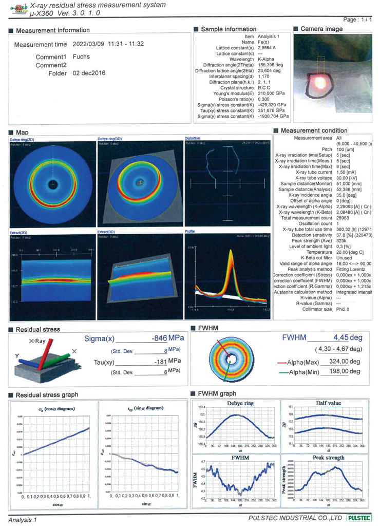
Regarding the Pulstec equipment, which is currently the only cos-alpha device on the market, a copy of the report of the obtained results is best, as all measurement values are available (Figure 24).

Figure 24.

Sample report.

3.12 Comparison between the sin2psi-2θ method and cos-alpha method

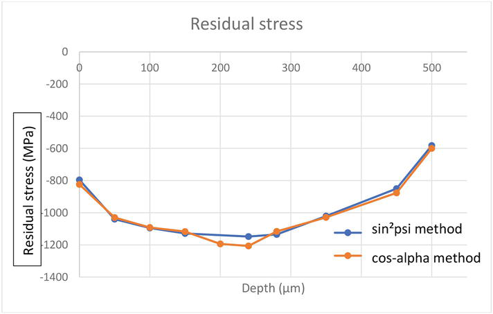
There is often a debate in the scientific community as to whether two methods provide the same results. Both techniques rely on Bragg’s law. However, surface roughness can influence the results and may not be the same in both methods. Therefore, the surface should be polished to eliminate surface roughness effects [17]. Initial investigations have been carried out, focusing on the material and residual stress state. For example, residual stress distribution in shot-peened components is isotropic in all directions, making it a very simple configuration. A list of the completed investigations can be found in [25]. Figure 25 illustrates the results of both methods measured on a shot-peened leaf spring.

Figure 25.

Residual stress distribution of a stress peened leaf spring [23].

Most comparisons find good agreement of the values determined using the cos-alpha method with the expected amount of stress and the sin²ψ-2θ-method (see [1, 2, 3, 4, 5]).

4. Conclusion

Compared with other X-ray stress determination methods, the cos-alpha method is usually faster, with a lower level of radiation exposure for the operator and highly mobile due to the measurement setup and weight of the equipment. Additionally, the cos-alpha method gives valuable information on the grain microstructure and helps to better interpret the measurement results. The high tolerance for setup errors enables even in good field and repeatable measurement results [5].

Currently, the cos-alpha method still lacks standardization, but some progress has been made to also implement the procedure in the available standards for X-ray stress analysis.

Appendix A: standards and guidelines

Since the method was only recently introduced in the market in the form of a commercially available device, the method still lacks standardization. There are, however, already some implementations of two standards that will be briefly discussed in this section. No further standards exist in the moment (Oct, 2023).

The VDA standard VDA 236–160 gives a short outline of the cos-alpha method. A future release of this standard is going to feature a longer paragraph on the method. A Japanese standard has also been published by the Society of Material Science Japan in the year 2020 (see [26] no English version is available at the moment Translated with Deep). This is a very detailed overview of the measurement principle and its application. The chapter overview gives an impression on the information provided in the standard.

Content of the Japanese standard:

Part I. X-ray Stress Measurement Standard by cos α Method.

Ferritic Steel Main text.

Chapter 1 General Provisions.

Chapter 2 General Information on Measurement Methods.

2.1 Principle of Measurement.

2.2 Measurement method.

2.3 Measuring conditions.

2.4 Stress value calculation method.

2.5 Measuring Apparatus.

2.6 Measurement Procedure.

Chapter 3 Standard Measurement Methods for Ferritic Steel Materials.

3.1 Object of measurement.

3.2 Characteristic X-rays and diffraction planes.

3.3 X-ray elastic constants.

3.4 Calculation of stress values.

Part II Ferritic steels Description.

Chapter 4 General Provisions.

Chapter 5 Measurement Methods General.

5.1 Principle of measurement.

5.2 Measuring methods.

5.3 Stress value calculation method.

Appendix A Methods for Measuring X-Ray Elastic Constants and Stress Constants.

Appendix B Rotational Measurements.

Appendix C Zero Stress Tests.

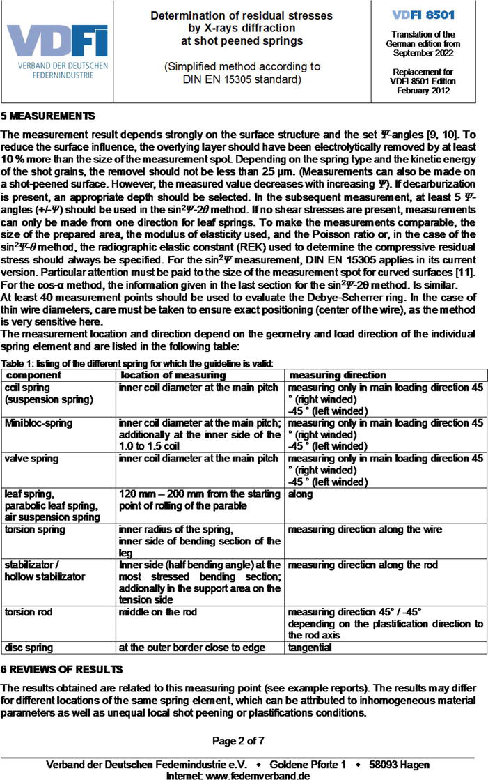
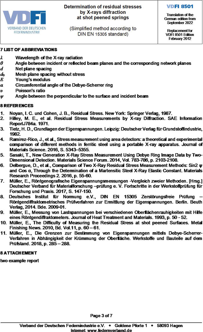
One of the earliest guidelines that outline how a measurement should be performed in Europe is the VDFI 8501 guideline from the German Spring Manufacturers Federation (VDFI: Verband der deutschen Federnindustrie). We present the guideline below, but we have omitted the sample reports that are briefly described in the in the reporting results section (courtesy of the VDFI) (Figures A1 and A2).

Figure A1.

Excerpt of the guideline for measuring springs (Page 2).

Figure A2.

Excerpt of the guideline for measuring springs (Page 3).

(The attachment of this standard is not relevant for the understanding. The above references belong to standard and the now following references belong to this chapter.)

References

1.Hiratsuka K, Sasaki T, Seki K, Hirose Y. Stress measuring system using image plate for laboratory X-ray experiment. In: The Abstracts of ATEM: International Conference on Advanced Technology in Experimental Mechanics: Asian Conference on Experimental Mechanics. The Japan Society of Mechanical Engineers; 2003. p. 377
2.Delbergue D, Texier D, Lévesque M, Bocher P. Comparison of two X-ray residual stress measurement methods: Sin2 ψ and cos α, through the determination of a martensitic steel X-ray elastic constant. In: Residual Stresses 2016. ICRS-10: 10th International Conference on Residual Stresses (ICRS10), Sydney, Australia, 3–7 July, 2016. Materials Research Proceedings. 2. Millersville, PA, USA: Materials Research Forum LLC; 2017. pp. 55-60
3.Kohri A, Takaku Y, Nakashiro M. Comparison of X-ray residual stress measurement values by cos α method and Sin2 Ψ method. In: Residual Stresses 2016. ICRS-10: 10th International Conference on Residual Stresses (ICRS10), Sydney, Australia, 3–7 July, 2016. Materials Research Proceedings. 2. Millersville, PA, USA: Materials Research Forum LLC; 2017. pp. 103-108
4.Spieß L, Matthes S, Grüning A. Röntgenographische Spannungsmessung - Vergleich von sin2ψ- und cos α-Verfahren. Berlin: Deutsche Gesellschaft für Zerstörungsfreie Prüfungen e. V., ZfP heute; 2020. pp. 39-41
5.Mueller E. Vergleich zweier röntgenografischer Verfahren zur Bestimmung von Eigenspannungen. In: Ilmenauer Federntag. Ilmenau: STZ Federntechnik; 2019. pp 59-65
6.Spieß L, Teichert G, Schwarzer R, Behnken H, Genzel C. Moderne Röntgenbeugung. Wiesbaden: Springer Fachmedien Wiesbaden; 2019
7.Tanaka K. The cosα method for X-ray residual stress measurement using two-dimensional detector. Mechanical Engineering Reviews. 2019;6:1. DOI: 10.1299/mer.18-00378
8.Ramírez-Rico J, Lee S, Ling J, Noyan IC. Stress measurement using area detectors: A theoretical and experimental comparison of different methods in ferritic steel using a portable X-ray apparatus. Journal of Materials Science. 2016;51:5343-5355
9.Kittel C. Introduction to Solid State Physics. 8th International ed. Hoboken, NJ: Wiley; 2005
10.Mueller E. The Debye–Scherrer technique—Rapid detection for applications. Open Physics. 2022;20(1):888-890
11.Lee S-Y, Ling J, Wang S, Ramirez-Rico J. Precision and accuracy of stress measurement with a portable X-ray machine using an area detector. Journal of Applied Crystallography. 2017;50(1):131-144
12.Chighizola CR, D’Elia CR, Weber D, Kirsch B, Aurich JC, Linke BS, Hill MR, Intermethod comparison and evaluation of measured near surface residual stress in milled aluminum, In: Experimental Mechanics 61 (2021) Nr. 8, S. 1309–1322
13.Mueller E. Die Grenzen zur Bestimmung von Eigenspannungen mittels Debye-Scherrer-Verfahren in Abhängigkeit der Krümmung der Oberfläche. In: Werkstoffe und Bauteile auf dem Prüfstand; 2017. Düsseldorf: Stahlinstitut VDEh; 2018. pp. 285-288
14.Maslowski LN. Korrekturfaktoren für die Bestimmung von Eigenspannungen an gekrümmten Oberflächen bei Röntgen-Diffraktometrie [thesis]. Germany: Bochum University of Applied Sciences; 2022
15.Mueller E. Die Bestimmung von Eigenspannungen an Grossbauteilen mittels Röntgendiffraktometrie mit Hilfe des Cos-α-Verfahrens. In: 54. Tagung des Arbeitskreises Bruchmechanik und Bauteilsicherheit - Bruchmechanische Werkstoff- und Bauteilbewertung: Beanspruchungsanalyse, Prüfmethoden und Anwendungen. Berlin: Deutscher Verband für Materialforschung und -prüfung e.V.; 2022. pp. 83-92
16.Mueller E. The difficulty of measuring the residual stress at shot peened surfaces. MFN (Metal Finishing News). 2010;2010(11):60-61
17.Volkswagen AG. Ferritische Eisenwerkstoffe Bestimmung von Eigenspannungs-Tiefenverläufen, PV 10052005. Wolfsburg, Volkswagen; 2005. p. 5
18.Holmberg J, Berglund J, Stormvinter A, Andersson P, Lundin P. Influence of local Electropolishing conditions on Ferritic–Pearlitic steel on X-ray diffraction residual stress profiling. Journal of Materials Engineering and Performance. 2023;(32):1-9
19.Wasniewski E, Honnart B, Lefebvre F, Usmial E. Material removal, correction and laboratory X-ray diffraction. Advanced Materials Research. 2014;996:181-186
20.Alkaisee R, Peng RL. Influence of layer removal methods in residual stress profiling of a shot peened steel using X-ray diffraction. Advanced Materials Research. 2014;996:175-180
21.Behler J. Develop and Verify shot peening processes. IST International Surface Technology. 2023;16(1):38-41
23.Bhandari P. Random vs. systematic error, Definition & Examples. Available from: https://www.scribbr.com/methodology/random-vs-systematic-error/ [Accessed: October 20, 2023]
24.Mueller E. Physik II - Vorlesung 1: Fehlerrechnung. YouTube, Available from: https://www.youtube.com/watch?v=Fegwu402YrM; [Accessed: August 16, 2023]
25.Mueller E. The long-term stability of residual stresses in steel. SN Applied Sciences. 2021;3(12):877
26.JSMS-SD-14-20. Standard for X-Ray Stress Measurement by the Cos α Method. Japan: The Society of Materials Science; 2020
Written By
Eckehard Müller and Jörg Behler
Submitted: 18 August 2023Reviewed: 25 August 2023Published: 21 February 2024