Perspective Chapter: Why Do We Care about Violating Bell Inequalities?

Abstract

High energy experiments present an exciting new regime in which to explore the violation of Bell inequalities by nature. There are two main reasons why one is interested in Bell inequality violation. The first is that—for suitable experimental configurations—Bell inequality violation can indicate the failure of the condition of Local Causality, which condition is a natural way of capturing the desideratum of no superluminal action-at-a-distance. The second is that Bell inequality violation is an Entanglement Witness. I review both of these reasons for interest, and suggest that high energy experiments plausibly involve the latter rather more than the former, at least as currently configured.

1. Introduction

Recently there have been both a number of proposals for, and actual experimental tests of, Bell inequality violation in high energy experiments (see e.g., [1, 2, 3]). This is an important new regime for exploring entanglement and Bell inequality violation, involving very different length-scales from the current state of the art in Bell experiments (compare [4]). It offers the promise of new insights into quantum correlations and entanglement at the femtometre scale, and will help us in our concrete understanding of the behaviour of relativistic quantum fields.

But at the same time, it is noteworthy that despite its now being nearly 60 years since Bell’s seminal paper [5], and despite the award of the 2022 Nobel prize to Aspect, Clauser and Zeilinger for their experimental work demonstrating Bell inequality violation, there is still considerable controversy over what Bell inequality violation really means, and why we should care about it [6, 7].

Here I will review the meaning of Bell inequalities and the significance of their violation, distinguishing two distinct broad areas of interest:

1. Tests of whether the world is nonlocal, or more precisely, is not locally causal [8], and

2. Tests of whether a multipartite system described by quantum mechanics is in an entangled state or not (that is, the use of Bell inequalities as entanglement witnesses [9]).

In the high energy Bell tests, the latter notion is certainly in play and it is important. As we shall see, however, it is an open question the extent to which the criteria for providing a test of the first kind are satisfied in high energy experiments.

2. Bell correlations and entangled states

For Schrödinger, entanglement was the characteristic feature of quantum theory, that feature which ‘enforces its entire departure from classical lines of thought’ [10]. Feynman, by contrast, insisted that it was the concept of superposition, as manifested in the two-slit experiment, that was ‘the heart of quantum mechanics. In reality, it contains the only mystery…’ [11]. Reassuringly, we need not see these two claims as being as much in dispute as one might initially suppose: for entanglement can be understood simply as genuinely multi-particle superposition.

Thus, given some system A with a Hilbert space ${\mathcal{H}}_A$ and a set of basis states $\left\{|{\varphi }_i⟩\in {\mathcal{H}}_A\right\},⟨{\varphi }_i|{\varphi }_j⟩={\delta }_{\mathit{ij}}$, then A is in a superposition with respect to that basis iff its state vector $\mid \psi ⟩\in {\mathcal{H}}_A$ is given by:

$$\mid \psi ⟩=\sum _i{c}_i\mid {\varphi }_i⟩,$$E1

where more than one of the coefficients $c_i$ is non-zero.

Now consider a second system, B, with ${\mathcal{H}}_B;\left\{|{\chi }_j⟩\in {\mathcal{H}}_B\right\},⟨{\chi }_j|{\chi }_k⟩={\delta }_{\mathit{jk}}$. The pair of systems AB will be (pure state) entangled iff their joint state $\mid \mathrm{\Psi }⟩\in {\mathcal{H}}_A\otimes {\mathcal{H}}_B$cannot be written as a product, i.e.:

$$\mid \mathrm{\Psi }⟩\ne \mid \varphi ⟩\mid \chi ⟩,$$E2

for any $\mid \varphi ⟩,\mid \chi ⟩$ in ${\mathcal{H}}_A,{\mathcal{H}}_B$, respectively. If the joint state could be written as a product $\mid \varphi ⟩\mid \chi ⟩$, then even though $\mid \varphi ⟩$ might be a superposition with respect to some basis of interest for ${\mathcal{H}}_A$, and $\mid \chi ⟩$ might be a superposition with respect to some basis of interest for ${\mathcal{H}}_B$, we would not have multiparticle superposition: each particle individually would merely be in its own superposition. By contrast if we have a state of the form:

$$\mid \mathrm{\Psi }⟩=\sum _i{c}_i\mid {\varphi }_i⟩\mid {\chi }_i⟩,$$E3

with more than one $c_i$ non-zero, then it cannot be written as a product, and we have genuinely multiparticle superposition: a superposition of the product basis $\mid {\varphi }_i⟩\mid {\chi }_i⟩$ for the two systems.

We can immediately see that something interesting is going on with an entangled state like (3).

Take a somewhat simplified case for illustrative purposes: suppose the states $\mid {\varphi }_i⟩$ corresponded to states with compact spatial support within a small width $\mathrm{\Delta }$ around a location which is i units along the x-axis (with a unit length being $>2\mathrm{\Delta }$, say), and similarly, suppose that the states $\mid {\chi }_i⟩$ corresponded to states with the same width but at a location $i+2$ units along the x-axis. Then if we think that being in an eigenstate of the operator corresponding to some physical quantity is both necessary and sufficient for a system’s having a definite value of that property, our pair of systems in the state given by (3) will definitely be two units of length apart from one another, whilst neither system A, nor system B, individually has any definite location of its own. This is a very striking, and non-classical, kind of holism about quantum property possession: the properties possessed by the whole system are not determined by properties possessed by the sub-systems, even for such a simple and important property as position. To take another, very familiar, example, consider the singlet state of a pair of spin-half particles:

$$\mid {\mathrm{\Psi }}^{-}⟩=\frac{1}{\sqrt{2}}\left(|\uparrow ⟩|\downarrow ⟩-|\downarrow ⟩|\uparrow ⟩\right).$$E4

This is of the form (3) and clearly an entangled state. In this case, the two spins are definitely in opposite directions, without there being a fact about which direction, if any, each individual spin is pointing in. Again: we have properties of the whole which are not determined by the properties of the parts, in a way which is not possible classically.

Even if we do not think that a system’s being in an eigenstate of the operator corresponding to some quantity implies that the system actually has a definite value of that quantity, but (as in some approaches to understanding quantum theory, e.g. [12]) restrict ourselves to the weaker claim that it merely implies that a suitable measurement interaction will give a particular result with probability one, entangled states remain strikingly non-classical and of great interest. An entangled state such as (3) is a pure state of the theory: it is not composed (in the theory) of a statistical mixture of more fine-grained states. Yet it will both give rise to non-trivial probabilities (i.e. those other than 0 and 1) for all observables for each system taken individually, whilst also providing correlations between measurement results on the two sides. This is not possible classically: in a classical probabilistic theory, pure states cannot give rise to correlations. (Consider two classical bits: we can only make a correlated state by producing a mixture of two of the pairs of bit values, e.g. by tossing a fair coin and producing (pure) bit values 01 on heads and 10 on tails, say).

The definition of pure state entanglement above can be generalised in two different directions: we can define entanglement for non-pure, i.e., mixed states, and we can define it for multipartite systems, i.e. those with a number of components $N>2$, rather than just for bipartite ($N=2$) systems.

A mixed state of a bipartite system AB, represented by a density operator ${\rho }_{\mathit{AB}}$, is an entangled state iff it cannot be written in the form:

$${\rho }_{\mathit{AB}}=\sum _i{\lambda }_i{\rho }_A^i\otimes {\rho }_B^i,$$E5

where ${\rho }_{A/B}^i$ are density operators on ${\mathcal{H}}_{A/B}$ respectively and the ${\lambda }_i$ are convex coefficients: real numbers $0\le {\lambda }_i\le 1$ which sum to one: ${\sum }_i{\lambda }_i=1$.

A state in the form (5) with only one term in the sum is called a product state; one with two or more terms is called seperable (or sometimes clasically correlated). If we include pure state density operators (${\rho }^2=\rho$) in our reckoning then this definition of entanglement covers both pure and mixed state cases.

The state ${\rho }_{1\dots N}$ of an N-party system is N-party entangled iff it cannot be expressed as a convex sum of the form:

$${\rho }_{1\dots N}=\sum _i{\lambda }_i{\rho }^i,$$E6

where each ${\rho }^i$ can be factorised into products states of less than N parties. An N-party system may be $M<N$-party entangled, even if it has no M-party subsystem whose reduced state is itself M -party entangled [13].

The GHZ state:

$$\mid {\mathrm{\Psi }}^{\mathrm{GHZ}}⟩=\frac{1}{\sqrt{2}}\left(|\uparrow ⟩|\uparrow ⟩\dots |\uparrow ⟩+|\downarrow ⟩|\downarrow ⟩\dots |\downarrow ⟩\right)$$E7

is a familiar example of an N-party state which is fully N-party entangled.

2.1 The Einstein-Podolsky-Rosen argument

Nowadays, entanglement is a workhorse of quantum information science, essential for entanglement-assisted communication (e.g. quantum teleportation), quantum computation, and quantum cryptography [14]. But it was first explicitly put to work by Einstein in his debates with Bohr on the completeness of quantum theory [15].

In these debates, Einstein would formulate thought experiments designed to illustrate that there was some knowable physical fact which a description according to the rules of quantum theory would leave out [16]. Bohr typically responded by arguing that the measurements involved in the putative experiments must be disturbing (due, as he was wont to say, to ‘the finiteness of the quantum of action’ [15, 17]) and hence they did not after all reveal that there were some knowable physical facts which the quantum description left out.

Einstein brilliantly realised that the correlations encapsulated in entangled states could transform this debate [18]. If we consider an experiment in which the measurement is performed on one half of a spatially separated entangled pair, and we ask about the physical features of the other half, then Bohr would be able to maintain his disturbance-on-measurement doctrine only at the cost of invoking some form of action-at-a-distance. The measurement on one side would have to disturb the physical features of the far side.

Thus the argument of the famous Einstein-Podolsky-Rosen (EPR) paper [19] was to the conclusion of a dilemma: either quantum theory is incomplete—it does not describe all the knowable physical features of systems—or it is nonlocal: it involves instantaneous action-at-a-distance. Einstein, for obvious reasons, preferred the first horn of the dilemma.

As formulated in the EPR paper (Einstein himself would prefer simpler, later, presentations [18, 20]) the argument used an important principle, the EPR criterion of reality:

‘If, without in any way disturbing a system, we can predict with certainty (i.e., with probability equal to unity) the value of a physical quantity, then there exists an element of reality corresponding to that quantity. ’[19]

Consider the singlet state (4) above, and suppose that Alice, in one lab, holds one half of a pair of systems in this state, whilst Bob, in a distant lab, holds the other. If Alice were to measure spin in the z-direction, say, she would get either the outcome spin-up with 0.5 probability, or the outcome spin-down, with 0.5 probability. Suppose she gets spin-up. As soon as she has her measurement result, she knows that a measurement on Bob’s system in the z-direction would now with certainty give a spin-down outcome. From the EPR criterion we can infer that there is an element of reality of Bob’s system corresponding to this spin value. Alternatively we might simply note that following Alice’s measurement, to get the correct probabilities for measurement results on Bob’s system, we now need to assign it the state $\mid {\downarrow }_z⟩$. Either way, the supposedly complete quantum state (4) misses something out: it does not include an element of reality corresponding to spin down in the z direction for Bob’s system, and it does not assign the state $\mid {\downarrow }_z⟩$. So either the quantum description is missing things out, or the result of Alice’s measurement is to change the features of Bob’s system, e.g., in the instantaneous change of the state of his system from ${\rho }_B=1/2(\mid \uparrow ⟩⟨\uparrow |+|\downarrow ⟩⟨\downarrow \mid )$ to $\mid {\downarrow }_z⟩⟨{\downarrow }_z\mid$.

Bohr’s reply to EPR [21] is generally felt to be somewhat obscure [15, 22, 23] but a summary version would be that—for all its plausibility—he rejected the EPR criterion of reality.

One simple way of taking this is as a rejection of the idea that the changing of the probabilities for the outcomes of measurements on Bob’s far system, given Alice’s nearby action, need correspond to the changing of any intrinsic physical feature of Bob’s system. (Nonlocal action, note, would require changes in the locally defined—the intrinsic—properties of the far system).

In turn, an extreme way of implementing this thought is to step back from the idea that the formalism of quantum theory, and in particular the quantum state, provides much in the way of description of the actual microphysical world in the first place. For example, if one took the (controversial) view that quantum states are no more than compendia of probabilities for the observable macroscopic results of measurement interactions, for ensembles of similarly prepared systems [12], and do not purport to describe microphysical reality, then one would not be troubled by the change in the state of Bob’s system from $1/2(\mid \uparrow ⟩⟨\uparrow |+|\downarrow ⟩⟨\downarrow \mid )$ to $\mid {\downarrow }_z⟩⟨{\downarrow }_z\mid$. Since quantum states, on this view, do not describe the actual microphysical properties of individual quantum systems, such a change in the state would not correspond to a change in the properties of any system, hence not to a nonlocal change. On the other hand, it might be felt that stepping back so far from quantum theory’s having descriptive microphysical content would be to throw the baby out with the bathwater.

2.2 Bell’s theorem

In any case: the EPR argument was, as we have seen, an argument about the content of quantum theory, over whether the theory was incomplete or was nonlocal. Bell changed things completely. His concern was not whether some particular theory (e.g. standard quantum theory) was nonlocal. His question was rather whether the world is nonlocal. That is, does any empirically adequate theory of the world—any theory which will account for the experimental results—have to include nonlocality within it?¹ He was able to address this question by beginning from a suitably theory-independent starting place.²

Thus let us frame the question of the existence of various correlations operationally. Suppose we begin with a pair of black boxes 1 and 2, where box 1 takes an input bit value $x=0,1$ and outputs a value $A=\pm 1$ with some probability distribution $P\left(A|x\right)$, and box 2 takes an input value $y=0/1$ and outputs a value $B=\pm 1$ with probability distribution $P\left(B|y\right)$ (Figure 1).

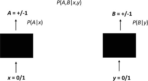
Figure 1.

Correlation boxes. For randomly chosen input values x, y we gather output values A, B and estimate the individual and joint probabilities $P\left(A|x\right),P\left(B|y\right)$ and $P\left(\mathit{AB}|\mathit{xy}\right)$ respectively.

Suppose that we run a large number of repeated trials using these boxes, choosing input values x and y randomly and independently of each other. Gathering the input and output data, we will be able to estimate the underlying probability distributions. Suppose furthermore that when we gather the statistics we find there to be correlations between the outputs of the boxes, so that:

$$P\left(\mathit{AB}|\mathit{xy}\right)\ne P\left(A|x\right)P\left(B|y\right).$$E8

We can explore the idea that these correlations are due, and due only, to some further variable $\lambda$ connecting the boxes. If they are, then when we condition on this further variable, the joint probability for A and B should factorise:

$$P\left(\mathit{AB}|\mathit{xy\lambda }\right)=P\left(A|\mathit{x\lambda }\right)P\left(B|\mathit{y\lambda }\right).$$E9

Call this the factorisability condition. We have been supposing that the input values x and y are chosen independently of each other. If they are, additionally, independent of the new variable $\lambda$ (too)

$$P\left(\lambda |\mathit{xy}\right)=P\left(\lambda \right),$$E10

a condition we may label $\lambda$-independence, then the joint probability for the outcomes can be expressed as:

$$P\left(\mathit{AB}|\mathit{xy}\right)=\int P\left(A|\mathit{x\lambda }\right)P\left(B|\mathit{y\lambda }\right)P\left(\lambda \right)\mathit{d\lambda }.$$E11

Call a joint probability which can be expressed in the form (11)Bell correlated.

If the probabilities for the behaviour of our boxes are Bell correlated, then a number of interesting inequalities—called Bell inequalities [5]—follow. For example, if we define the expectation value (equivalently, the correlation function) for the outputs of our boxes for various inputs as:

$$E\left(x,y\right)=\sum _{\mathit{AB}}\mathit{AB}P\left(\mathit{AB}|\mathit{xy}\right),$$E12

then one such is:

$$\mid E\left(x=0,y=0\right)+E\left(x=0,y=1\right)+E\left(x=1,y=0\right)-E\left(x=1,y=1\right)\mid <2.$$E13

This is known as the Clauser-Horne-Shimony-Holt (CHSH) inequality [25]; it is a particular Bell inequality. Nowadays, a menagerie of different Bell inequalities is available, for example allowing different numbers of inputs and outputs, and numbers of boxes greater than two [26]. They all follow from the assumption that the salient joint probabilities can be expressed in the form (11).

But why should we care about this? Why should we care whether our boxes are Bell correlated or not; whether they satisfy a Bell inequality or not?

We care when we embed the boxes in a relativistic spacetime, and the choice of x and the outcome A occur at spacelike separation from the choice of y and the outcome B.

Start with the idea that correlations should be explicable, and start with the idea that:

‘The direct causes (and effects) [of events] are nearby, and even the indirect causes (and effects) are no further away than permitted by the velocity of light. ’[27]

This is Bell’s principle of Local Causality. It incorporates both the idea that causal relations are mediated (a causal link between distant events a and b will be made up of a causal chain of events between a and b, so the causal link does not obtain at a distance) and the constraint from relativity theory that the speed of light is the upper bound on the propagation of causal influence.

We need to formulate the principle mathematically to deploy it in our theories. This Bell did as follows [8, 27]:

If we consider an event A in spacetime (an event such as one our boxes producing a particular output on a particular occasion), then a full specification (or a sufficient specification) M of facts on a spacelike hypersurface through the past lightcone of A will render facts N associated with any other region of spacetime probabilistically irrelevant to A (see Figure 2). Thus:

Figure 2.

Local causality. A sufficient specification of facts on the surface M renders facts within N probabilistically irrelevant to the event A: $P\left(A|\mathit{MN}\right)=P\left(A|M\right)$.

$$P\left(A|\mathit{MN}\right)=P\left(A|M\right).$$E14

This is the formal statement of Local Causality.

Applying it to the case—call it the standard configuration—in which we have embedded our correlation boxes within spacetime, with the choice of x and the output A at spacelike separation from the choice of y and the output B, and with $\lambda$ a full or sufficient specification of facts in a spacetime region cutting through the past light cones of A, B, including where they overlap (see Figure 3), Local Causality will imply the factorisability condition (9).³

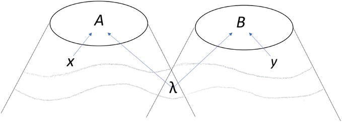
Figure 3.

A spacetime picture of the Bell experiment in standard configuration. $\lambda$ specifies facts in a spacetime region cutting through the union of the past light cones of A and B, including where they overlap.

Given too that x and y can be taken as free variables—or sufficiently free variables (we will return to this)—$\lambda$-independence will also hold, and so the CHSH inequality will follow for the outputs of our boxes.

Bell’s theorem is the claim that correlations in a standard-configuration experiment satisfying Local Causality and $\lambda$-independence will also satisfy a Bell inequality. It follows that any theory which predicts that the results of correlation experiments in standard configuration can violate a Bell inequality must also violate Local Causality, $\lambda$-independence, or both.

We know that the CHSH inequality has been shown to be violated for high quality experiments in standard configuration (e.g. [4, 28]), and we very reasonably believe that in these experiments, it was possible to choose the input variables x and y independently. Accordingly it seems we must conclude that Local Causality fails.

This is often taken to lead to two further conclusions (very distinct from one another):

• Quantum mechanics is nonlocal; and

• The world is nonlocal.

3. Now for some controversy

These conclusions are remarkable in reach and content, but the path that led to them seems clear enough. How can there be any controversy regarding the meaning of Bell inequality violation?

The simplest place to begin is by noting that certain ways of understanding quantum theory would seem already to provide counterexamples to the last two conclusions of the previous section.

Note to begin that we did not (as Bell was himself very aware) need experimental violation of Bell inequalities to conclude that quantum theory is not locally causal. The quantum probabilities for the correlation experiments are given by:

$$P\left(\mathit{AB}|\mathit{xy\lambda }\right)=⟨\mathrm{\Psi }|P_x^A\otimes P_y^B|\mathrm{\Psi }⟩,$$E15

where $P_x^A$ is the projector (or more generally, positive operator) associated with the value A for measurement of quantity x, and $P_y^B$ similarly, and $\lambda$ captures that we have prepared state $\mid \mathrm{\Psi }⟩$ for our bipartite system. It is automatic that this quantity will not factorise whenever $\mid \mathrm{\Psi }⟩$ is entangled.

Meanwhile, approaches to quantum theory which take its content to be mainly operational—capturing the statistics of macroscopic measurement results, say, rather than describing physical features of quantum sytems—or that otherwise step back from the detailed description of a mind-independent physical world can still count as local. There are even ways—at least one—of taking quantum theory to be descriptive of the detailed microphysical features of the world and of individual quantum systems whilst still remaining local: the Everett (Many Worlds) interpretation of the theory is generally taken to be local [24, 29].

This raises the question of how failure of the specific condition of Local Causality relates to the presence of nonlocality, and especially to the presence of any nonlocality we might find worrying or problematic.

It is helpful to note that we can distinguish between two different notions, each of which can be thought to fall under the more general heading of ‘nonlocality’ (the distinction goes back to Einstein in fact [20], though my terminology is not quite his):

• Dynamical nonlocality—there are changes in locally defined (intrinsic) properties in some region due to spacelike happenings elsewhere. (This is a notion of genuine superluminal action).

• Kinematical nonlocality—the states assigned to unions of spacetime regions are not determined by the states assigned to the individual regions. (This is often known as the failure of separability).

Certainly in quantum mechanics when we have a failure of separability in the sense that we have an entangled state for a pair of systems, and when those two systems are spatially separated, we will also have a failure of separability in the sense of kinematical nonlocality. Perhaps other, post-quantum, theories might similarly be kinematically nonlocal. Kinematical nonlocality is certainly a striking and non-classical feature, but it seems perfectly coherent theoretically (it is an actual feature in quantum theory) and in and of itself it does not give rise to any problems of consistency with relativity (though we should note that a kinematically nonlocal theory will still need to allow a rich-enough range of locally defined properties given by the states of individual regions, as is achieved in quantum theory via use of the reduced density operator [30]). If kinematical nonlocality can be combined with the absence of any dynamical nonlocality then we may have a perfectly satisfactory theory, consistent with relativity, and perhaps one which can violate a Bell inequality unproblematically.

On the other hand, Bell’s intuitive prose statement of Local Causality did seem to capture our notions of dynamical locality consistent with relativity, and his reasoning from this statement to the factorisability condition seems simple and sound. What, if anything, can have gone wrong with it?

To make this question more pointed, suppose that we did try to appeal to a mere failure of kinematical locality, rather than a failure of dynamical locality, to explain Bell-inequality violation. How would this failure of kinematical locality actually help? We may grant there to be non-separable features in the joint past of Alice and Bob’s correlation experiments, but surely we can just condition on these and include them within $\lambda$ [31]? Then a Bell inequality should still hold, and kinematical nonlocality will not have helped us to violate it.

3.1 Looking at the examples

To unpick these puzzles, let us look a little more closely at how the proposed examples of local understandings of quantum theory work. We can discern three kinds of example.

The first kind of example we are already familiar with from what I called the ‘extreme’ way of offering a response to EPR in wake of Bohr. It is the kind of view which retreats from the idea that quantum theory, and the quantum state, provide us with means of describing the microphysical world. Instead the formalism of the theory is seen as a device for organising our experimental interactions with the world, and quantum probabilities only pertain to the behaviour of measuring devices which can be characterised non-quantum mechanically and at the macroscopic level. The only role of the quantum state is to furnish these probabilities; it does not describe actual features of quantum systems. Such views [12] can be called operationalist (foregrounding operational procedures in the lab) or anti-realist in the sense that they depart from a scientific realist conception of our physical theories. In a scientific realist conception, the aim of science is to provide us with a literally true description of the what the mind-independent world is like in both its directly observable and non-directly observable features, and as applied to quantum theory, it would require us to interpret at least a large part of the quantum formalism as directly representing facts about the microphysical systems from which the world is built.

In a sufficiently operationalist or anti-realist interpretation of a theory, the notion of (dynamical) locality will itself be given a suitably operationalist understanding. Since the theory is not in the business of describing microphysical goings-on in individual runs of an experiment, but rather in the business of codifying statistical features, non-microphysically characterised, of repeated runs of experiments, the notion of dynamical locality will be spelt out in statistical, operational, terms: a theory will be (operationally) nonlocal iff it is signalling, where a theory is signalling iff operational procedures confined to one spacetime region produce a change in the statistics for measurement outcomes in a spacelike region.

Quantum theory itself is rather obviously non-signalling since the reduced density operator for a far system is unchanged by any operation one can perfom on a nearby system. A sufficiently operationalist interpretation of quantum theory, therefore, will—by the relevant estimation—count as dynamically local despite predicting Bell inequality violation.

Notably, such an approach does not explain how Bell inequality violation comes about in experiments, it just asserts that it does. It gives-up on the idea of explaining physically how correlated measurement results turn out as they do on individual runs of an experiment, as part more broadly of relinquishing descriptive ambitions for quantum theory. Remaining fastidiously aloof from describing microphysical systems, it will remain equally aloof from causal description of events involving those systems, hence Bell’s prose statement of the principle of Local Causality above will not apply straightforwardly, if at all. But as remarked before in the context of the EPR argument, taking so stringently thin a notion of the content of quantum theory as this may be depriving ourselves of too much that we need.

The second kind of example may agree with the prose statement of Local Causality, but instead raise trouble for the mathematical expression of the principle in terms of probabilities as in Eq. (14) and Eq. (9). In particular, one might offer a notion of probability according to which changes in the probabilities assigned by Alice to the possible results of measurements on Bob’s distant system do not count as changes in any objective, or in any localised, feature of his system. If changes in the probabilities pertaining to a system need not correspond to changes in objective or in localised features of the system, then the inference from changes in the probabilities to causal consequences in the world is rendered shaky.

It is tempting to think that there is a single correct, best, probability distribution for what the results of measurement on a given system should be, a probability distribution fixed by the features of the system and its immediate surroundings (perhaps including the features of any measurement device with which it is about to interact). In the quantum case, it is very tempting to think that this single correct, best, probability distribution is given by what the correct quantum state (pure or mixed) that this system should be assigned is.

But it might be argued, as in [32, 33] that there is no single set of probabilities which should be assigned to a given system; the physical features of a system, or more generally, the physical features of the world in the past light cone of a system, need not determine a single, univocal, probability for the results of measurement on that system. It will follow that there is not a single quantum state that should be assigned to a system either. Thus Alice following her spin measurement on her half of the entangled pair shared with Bob correctly assigns to Bob’s system the pure state $\mid {\downarrow }_z⟩$, but this assignment is not made correct by any feature intrinsic to (locally defined for) Bob’s system; it is made correct by what Alice has learnt at her location. Bob, correctly, and unimprovably (for now) at his location, not missing any physical feature intrinsic to his system, continues to assign the mixed state to his system.

In this kind of view, the full specification of physical facts on some spacelike hypersurface do not determine univocal and ideally best probabilities for each event on future spacelike hypersurfaces, so we cannot straightforwardly draw causal inferences from the probabilities assigned to an occurence changing when conditioned on facts pertaining to a spacelike separated region.

In [32, 33] probabilities (and quantum states) are objective, even if they are not univocal (because relational). A rather different picture is given in QBism [34], where again there are not univocal probabilities, and there are not unique quantum states for systems, but this time because probabilities (and quantum states) are viewed as subjective, in the sense of being expressions of individual agents’s degrees of belief. Again, this renders the probabilistic formulation of Local Causality as ineligible to express causal notions.

The third example is the particular concrete example given by the Everettian (Many Worlds) approach to quantum mechanics and it is quite unlike the first two kinds of example. Unlike these, in the Everettian approach, the quantum state (of the universe!) is unique, objective, and intended to be part of the detailed description of individual quantum mechanical systems. It is a thorough-going scientific realist approach to understanding quantum theory. But, it is generally held to be a dynamically local theory, indeed it will satisfy the prose statement of Local Causality, since in Everett, the state of any spacetime region will be fixed by the state on a spacelike surface cutting the past light cone of that region.

A number of tightly-interconnected factors seem to be involved in the Everett approach being able to violate Bell inequalities whilst remaining dynamically local:

1. Though the quantum state is real in the sense of playing a central role in describing real features of the world, it does not collapse on measurement, so there are no dynamically nonlocal changes in the state. Instead the state evolves by unitary dynamics given by a local Hamiltonian.

2. Apart from some background spacetime structure, all the remaining physical ontology (physical features of the world) supervenes on the quantum state and its evolution. (Nothing extra is added, such as hidden variables which might need to be pushed-about dynamically nonlocally.)

3. The theory is emphatically kinematically non-local, since entanglement between different spatially separated regions is generic.

4. There is non-uniqueness of measurement outcomes (different outcomes of a given measurement, in different worlds which have branched from the measurement). We do not need to guarantee single correlated outcomes on a given run of the experiment, at the expense of other possible outcomes: all the outcomes are realised.

It is an interesting open question whether any theory which is suitably scientific realist, which is dynamically local, which is kinematically nonlocal, and yet which can violate a Bell inequality (without $\lambda$-dependence), is also one in which uniqueness of measurement outcomes will fail. That is, do the features which co-occur in the Everett interpretation have to co-occur?

In any case: the clearest lesson from reflecting on the Everett example seems to be that in a theory which is kinematically non-local, the probabilistic formulation of Local Causality may again not be an appropriate way of expressing the prose formulation of Local Causality [24].

3.2 Summing-up this controversy

Though they incorporate, or express, a range of very different philosophical approaches, perhaps the simplest, quick, way to understand these controversies is to discern an ambiguity (deliberately planted there) in my earlier statement of Bell’s theorem. I said that the theorem was the claim that correlations in a standard-configuration experiment satisfying Local Causality and $\lambda$-independence will also satisfy a Bell inequality. But which version of Local Causality? The initial, intuitive, prose version? Or the mathematical formulations, Eqs. (9) and (14)? No one could deny the content of the theorem if we meant the latter. But as we have seen, there are a number of routes by which one might endorse the prose version of the principle, but not agree with its mathematical formulation, thus not agree with the claim, if Local Causality in the prose formulation is intended.

Still: the class of theories for which the mathematical formulation is a good way of expressing Local Causality is very broad and important. So the claim that Bell inequality violation in nature shows that Local Causality, as mathematically expressed, is not true, is still very deep, remarkable, and powerful.

3.3 ‘Local causality’ vs. ‘local realism’

It is rather common to find Bell’s results discussed under the heading of ‘Local Realism’ instead of ‘Local Causality’. This alternative terminology may perhaps be traced back to [35, 36], but it can be highly, and distractingly, controversial. For some, asserting that Bell inequality violation (for standard configuration experiments, etc.) rules out Local Realism invites the prospect that locality might be salvaged by jettisoning a(n allegedly atavistic) realism assumption. For others, such a contention must be quite mistaken, for Bell’s reasoning did not and need not make any appeal to any assumptions beyond locality (Local Causality) itself [37, 38, 39].

There is some truth in both contentions, but there is no doubt that ‘Local Causality’ is the better terminology, for it does not invite the confusions that ‘Local Realism’ does.

We have already seen that some dialling-down of realist, descriptive, ambitions for physics does allow scope for evading inferences to the presence of dynamical nonlocality (action at a distance) both in the context of the original EPR argument (recalling the tenor of Bohr’s response), and in one of the routes we explored for resisting the idea that the mathematical and the prose formulations of Local Causality aptly express conditions for dynamical locality in all contexts. So some realist commitment is involved as part of the background of Local Causality’s expressing an interesting physical feature. But what is the realism in Local Realism supposed to be?

For some it is just a generic commitment to the notion of scientific realism along the lines introduced above. Thus Clauser and Shimony: ‘Realism is a philosophical view, according to which external reality is assumed to exist and have definite properties, whether or not they are observed by someone.’ [35]. On other occasions, realism is taken to be the logically much stronger—or more specific—view that all physical quantities (e.g. all quantities represented by self-adjoint operators in quantum mechanics) have a definite value for what the result of measuring them on some occasion would be, even if they were not in fact measured on that occasion [36]. The latter is a stronger view since it commits to there being hidden variables which are deterministic (fixing definite measurement outcomes), whereas in the former view it could be that there are independently existing properties of the world but that they only (in general) furnish non-deterministic probabilities for measurement outcomes. Further, the latter reading suggests definite values for all physical quantities simultaneously, where one might take the external world to have real mind-independent features at all times, but perhaps only for a subset of the physical quantities.

The strong view (realism as deterministic hidden variables) is too narrow. Local Causality covers a broader range of theories than this (and it needs to, to be applicable to realistic experimental scenarios). But if we relax merely to the broader view (scientific realism as applied in the quantum context) then we find examples of theories which are (dynamically) local and realist in this sense, but which can violate Bell inequalities: the Many Worlds approach. So locality and realism (in this broader sense) do not entail Bell inequalities; while locality and realism (taken in the narrower sense) does not cover all cases. We should simply drop ‘Local Realism’ and stick with ‘Local Causality’.

4. Back to $\lambda$-independence

If our correlation experiments were not in standard configuration, then it would be easy for them to produce Bell inequality violating results without there needing to be any failure of local causality, or any other non-classical funny-business. For example, if the setting—x, say—on one side was not at spacelike separation from the setting or outcome on the other, then there would be plenty of time for a classical sub-luminal, or a lightlike, channel to connect the two sides. Bob’s box would then be able to take both x and y as inputs, and locally mimic failure of local causality. (The response function which captures the behaviour of Bob’s box can now be of the form $P\left(B|x,y,\lambda \right)\ne P\left(B|x,\lambda \right)$ consistently with local causality.) This additional channel connecting the two sides of the experiment might not be obvious to us, but it could certainly be there. Requiring that the experiment be in the standard configuration rules out there being any such channel, on pain of inconsistency with relativity.

It is also extremely important that there actually be a choice of x and y values when the experiment is run. If x and y took the same fixed values across all runs of the experiment then we would not have any interesting correlations. Any correlations in the outputs ($P\left(\mathit{AB}\right)\ne P\left(A\right)P\left(B\right)$) could readily be accounted for by a purely locally causal mechanism. More subtly, if x and y choices were made on each run, but we happened to know in advance what they would be, it would again be possible to mimic failure of local causality locally: we could adjust the other input to the boxes, via $\lambda$, to make it look as if local causality were failing when it was not. This brings us back to the question of $\lambda$-independence.

It will be recalled that $\lambda$-independence ((10) above) was an essential ingredient in arriving at Bell-correlations ((11) above) and thus in deriving Bell inequalities. We are used to the idea that we can often have a good deal of control over at least some of the parameters which are involved in our experiments. We are also used to the idea that, in general, separate systems will not be correlated with one another unless they have had some explicit interaction in the past, often, in the recent past. Accordingly, if when constructing our correlation experiment we have taken pains that the process by which the x input value is selected is independent of other things, and the process by which the y input value is selected is independent of other things, then it will seem reasonable to assume a) that x and y are not correlated with each other (in fact we can explicitly check whether $P\left(\mathit{xy}\right)=P\left(x\right)P\left(y\right)$) and b) that, crucially, they are not correlated with anything else important for the results of the experiment. With these precautions, then, $\lambda$-independence seems a safe assumption.

On the other hand, if this condition fails, then locally causal theories could produce arbitrary correlations—whether the quantum correlations, or even stronger correlations, which maximally violate the CHSH inequality (the Popescu-Rohrlich correlations [40]). To see this, let us consider a simple example.

Suppose we have a theory which is deterministic in the sense that specification of all the facts on a spacelike hypersurface which cuts through the past light cone of some event fixes all the facts to the future of that surface within the lightcone in question. By construction such a theory will be locally causal. It will also automatically violate $\lambda$-independence. To see this, consider that in such a theory both x and y will be functions of $\lambda$—call them $f\left(\lambda \right)$ and $g\left(\lambda \right)$ respectively. Then we can consider the set ${\mathrm{\Lambda }}_{\mathit{xy}}$ of all those values of $\lambda$ which would give rise to some specific x, y pair:

$${\mathrm{\Lambda }}_{\mathit{xy}}=\left\{\lambda |f\left(\lambda \right)=x,g\left(\lambda \right)=y\right\}.$$E16

Given some specific x, y in some run of the experiment, then, $\lambda$ in that run will be constrained to lie within ${\mathrm{\Lambda }}_{\mathit{xy}}$, which is a strict subset of the set $\mathrm{\Lambda }$ of all values of $\lambda$, which means that $\lambda$-independence fails. Knowing the values of x, y we know that $\lambda$ must be within a specific subset of values. Letting ${\chi }_{\mathit{xy}}$ be the characteristic function of the set ${\mathrm{\Lambda }}_{\mathit{xy}}$ (giving value 1 if $\lambda \in {\mathrm{\Lambda }}_{\mathit{xy}}$ and 0 otherwise), we have that:

$$P\left(\lambda |\mathit{xy}\right)=\frac{{\chi }_{\mathit{xy}}\left(\lambda \right)P\left(\lambda \right)}{P\left(\mathit{xy}\right)}\ne P\left(\lambda \right).$$E17

With the $\lambda$-dependence of this deterministic theory in hand, we can now see how to produce arbitrary correlations (this kind of construction seems first explicitly to have been noted, for quantum correlations, in [41]). We just need to put an appropriate probability distribution over the initial set of λs.

Note that in this theory, not only x and y but also the outcomes A and B will be functions of $\lambda$. We can thus further refine the ${\mathrm{\Lambda }}_{\mathit{xy}}$ with a partition:

$${\mathrm{\Lambda }}_{\mathit{xy}}=\bigcup _{\mathit{AB}}{\mathrm{\Lambda }}_{\mathit{xy}}^{\mathit{AB}},$$E18

where the ${\mathrm{\Lambda }}_{\mathit{xy}}^{\mathit{AB}}$ are the sets of all $\lambda$ values which produce the specific values x, y, A, B. (Note, ${\mathrm{\Lambda }}_{\mathit{xy}}^{\mathit{AB}}\cap {\mathrm{\Lambda }}_{x^{\prime }{y}^{\prime }}^{A^{\prime }{B}^{\prime }}=\varnothing$).

Taking ${\chi }_{\mathit{xy}}^{\mathit{AB}}$ to be the characteristic function of the set ${\mathrm{\Lambda }}_{\mathit{xy}}^{\mathit{AB}}$, the joint probability $P\left(\mathit{\text{ABxyλ}}\right)$ will be given by:

$$P\left(\mathit{\text{ABxyλ}}\right)={\chi }_{\mathit{xy}}^{\mathit{AB}}\left(\lambda \right)P\left(\lambda \right).$$E19

Suppose that it is the quantum correlations which we want to recover. Then we need merely postulate a $P\left(\lambda \right)$ which is such that the correct weight gets given to the sets ${\mathrm{\Lambda }}_{\mathit{xy}}^{\mathit{AB}}$. Thus we choose $P\left(\lambda \right)$ such that:

$$P\left(\lambda \in {\mathrm{\Lambda }}_{\mathit{xy}}^{\mathit{AB}}\right)=\int {\chi }_{\mathit{xy}}^{\mathit{AB}}\left(\lambda \right)P\left(\lambda \right)\mathit{d\lambda }=⟨\mathrm{\Psi }|P_x^A\otimes P_y^B|\mathrm{\Psi }⟩P\left(\mathit{xy}\right).$$E20

The correlation probabilities in this theory will be given by:

$$P\left(\mathit{AB}|\mathit{xy}\right)=\int \frac{{\chi }_{\mathit{xy}}^{\mathit{AB}}\left(\lambda \right)P\left(\lambda \right)}{P\left(\mathit{xy}\right)}\mathit{d\lambda }.$$E21

For the weights on ${\mathrm{\Lambda }}_{\mathit{xy}}^{\mathit{AB}}$ given by $P\left(\lambda \right)$ satisfying (20) we will immediately obtain $⟨\mathrm{\Psi }|P_x^A\otimes P_y^B|\mathrm{\Psi }⟩$ as desired. By choosing different weights on the ${\mathrm{\Lambda }}_{\mathit{xy}}^{\mathit{AB}}$ we can obtain any desired correlations.

The $\lambda$-dependence of this deterministic theory was of a rather strong kind, with $\lambda$ fixing x and y. It is also possible to pursue the more subtle question of how little $\lambda$-dependence is required in order to reproduce certain correlations locally causally. For example [42] shows that at most one bit of correlation (as measured by the mutual information) between $\lambda$ and one of the measurement settings is sufficient in order to be able to reproduce any correlations which could be generated by quantum measurements on a singlet state (see also [43]). In the other direction, interestingly, [44] shows that if one’s theory retains a little $\lambda$ independence, in the sense that given λs do not absolutely rule out particular x, ys, then there is a Bell inequality which would be violated for a less than maximally entangled quantum state, but which this $\lambda$-dependent theory would not be able to violate.

4.1 Effective $\lambda$-independence

The discussion so far of the $\lambda$-dependence of the deterministic theory leaves us with something of a puzzle. Earlier we noted that, having taken care to apply certain precautions, it would be perfectly reasonable to believe that $\lambda$-independence was satisfied for one’s experiment in standard configuration. But as we have just seen, if there is an underlying deterministic theory, then $\lambda$-dependence is obligatory. And it seems a perfectly reasonable thought that there might be some (perhaps as yet to be discovered) deterministic theory underlying quantum theory.

The key to resolving this conundrum is to recognise that what is important is effective$\lambda$-independence, as opposed to what might be called absolute or fine-grained$\lambda$-independence. (I take this to be one of the key lessons from—and an area of agreement within—the exchange between Bell and Clauser, Horne and Shimony [45].)

When considering the behaviour of some physical system—for example one of our black boxes—it may well be (at least for the sake of argument) that there is some fully deterministic theory in the background, which gives us a detailed $\lambda$ which is sufficient entirely to fix the system’s behaviour. Yet that physical system may in a certain sense be insensitive to $\lambda$. That is, although $\lambda$ fully fixes the behaviour, the system might behave in much the same way, or exactly the same way, for a range of values of $\lambda$. In other words, the behaviour of the system may best be characterised as responsive to some coarse-grained variables, corresponding to some coarse-graining of $\mathrm{\Lambda }$.

Let us introduce the notation $\overline{\lambda }$ for new variables given by some minimal coarse-graining of $\mathrm{\Lambda }$ (e.g., averaging values of $\lambda$ within some small $\mathrm{ϵ}$-volume of $\mathrm{\Lambda }$). Considering now the boxes in our correlation experiment, suppose them to be governed by a locally causal theory; their behaviour will be captured by the response functions:

$$P\left(A|\mathit{\text{Bxyλ}}\right)=P\left(A|\mathit{x\lambda }\right),\text{and}$$E22

$$P\left(B|\mathit{\text{Axyλ}}\right)=P\left(B|\mathit{y\lambda }\right).$$E23

Suppose now that the boxes are insensitive to fine-grained $\lambda$. There will be some coarse-grained $\overline{\lambda }$ which screens-off $\lambda$ in the response functions:

$$P\left(A|x\overline{\lambda }\right)=P\left(A|\mathit{x\lambda }\right);$$E24

$$P\left(B|y\overline{\lambda }\right)=P\left(B|\mathit{y\lambda }\right).$$E25

Now it may be that at this coarse-grained level, $\overline{\lambda }$-independence will hold—$P\left(\overline{\lambda }|\mathit{xy}\right)=P\left(\overline{\lambda }\right)$—even if $\lambda$ independence does not. Then we will again have Bell correlated joint probabilities, and Bell inequalities will hold for our locally causal theory:

$$P\left(\mathit{AB}|\mathit{xy}\right)=\int P\left(A|x\overline{\lambda }\right)P\left(B|y\overline{\lambda }\right)P\left(\overline{\lambda }\right)d\overline{\lambda }.$$E26

Say that effective$\lambda$-independence holds, iff there is some minimally coarse-grained $\overline{\lambda }$ which screens-off $\lambda$ in the measurement response functions and for which $\overline{\lambda }$-independence holds.

Effective $\lambda$-independence can certainly hold in a deterministic theory, and in the circumstances relevant to our experiment in standard configuration we would expect it to do so. Reflect that many and various different processes could be selected which produce the x and y input values for the experiment (and we can check to see whether it makes any difference to the presence of Bell-inequality violation which process is used). These processes could be of the kind where we have very good reason to believe that the dynamics (whatever it is) leading-up to the production of the value is extremely complicated (as for example in a pseudo-random-number-generator), so that an exact specification of the final state of the choosing-device would be necessary to determine its initial state, whilst the value produced itself is a very coarse-grained function of the final state of the choosing-device. In this circumstance, we can envisage that if there is an underlying deterministic theory, its sets ${\mathrm{\Lambda }}_{\mathit{xy}}$ are highly fibrillated and interwoven with one another. Then knowing the exact $\lambda$ would still fix which ${\mathrm{\Lambda }}_{\mathit{xy}}$ we were in. But even a slightly coarse-grained $\overline{\lambda }$ would not pin down any ${\mathrm{\Lambda }}_{\mathit{xy}}$: within the small $\mathrm{ϵ}$-ball some (approximately) equal-measured subset of each ${\mathrm{\Lambda }}_{\mathit{xy}}$ might be present. Thus $\overline{\lambda }$-independence would hold.

Important as it is, this is not enough for effective $\lambda$-independence to hold. For that we also need that $\overline{\lambda }$ screens-off $\lambda$ in the response functions. However, given the enormous variety of ways (ways which we can to some extent choose between), and the enormous complexity of ways (which we can to some extent ensure), in which any fine-grained $\lambda$s can be connected to x and y values, it would be extraordinary if the response functions were always sensitive to the fineness of grain of $\lambda$ required to fix x and y. In other words, it would be extraordinary if $\overline{\lambda }$ did not screen-off $\lambda$ in the response functions, and thus effective $\lambda$-indepedence hold. (Plausibly, it would be far more extraordinary than Local Causality’s failing.)

Bell in [46] talks about input x and y variables, when they are produced by plausible randomisation processes, being ‘sufficiently free variable[s] for the purposes at hand’. I take the notion of effective $\lambda$-independence just outlined to be a way of capturinging this notion of ‘sufficiently free’. There may be some description (e.g. the envisaged underlying deterministic one) in which x and y are not free variables, since they are correlated with, or caused by, something else. But that need not stop them being effectively, or sufficiently, free; and the degree of coarseness of grain of $\lambda$ which both screens-off $\lambda$ in the measurement response functions and delivers $\overline{\lambda }$-independence captures the relevant metric for sufficient freedom.

4.2 The question of $\lambda$-independence in the case of high energy experiments

So far, then, we have reassured ourselves that in the standard configuration for the correlation experiment, and if one has taken trouble that the procedures for selection of x and y values are one from some number of suitably randomising procedures—or otherwise give us a high degree of confidence that the selection processes are independent of other aspects of the experiment—we may be confident that $\lambda$-independence, or effective $\lambda$-independence, holds.

It is sometimes suggested, however, that there may be special reasons even so why (effective) $\lambda$-independence might fail, thus allowing us to avoid the conclusion that the world is not locally causal, despite Bell inequality violation. Such special reasons might include the thought that backwards causation might be possible, so that we should not rule out the possibility that Alice and Bob selecting their x and y values could affect the value of $\lambda$ in the past (e.g. [47, 48]) or that a particular form of deterministic hidden variable theory might naturally give rise to $\lambda$-dependence [49]. In each of these cases (as also in [50]) we face the question of whether there is more reason to believe that these special reasons obtain than to believe that effective $\lambda$-independence does. Given the strength of the general physical grounds for believing effective $\lambda$-indpendence obtains, the general view is against these special reasons.

Throughout our discussion of (effective) $\lambda$-independence, however, it was extremely important that the processes which produced the selection of x and y values were separately identifiable and understandable to the extent that we could have confidence that the values produced were (at least effectively) independent of each other and of other features which might be important in the experiment. By controlling and probing the behaviour of these processes, we could come to a very high degree of confidence that such independence obtains. In terms of a causal diagram (rather than just a spacetime diagram) where arrows indicate the presence of causal influence and the absence of arrows its absence, we need a causal structure as given in Figure 4a.

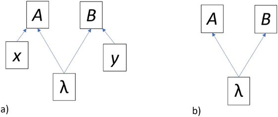
Figure 4.

Causal diagrams for correlation experiments. In a) we have standard configuration with x and y values independently selected, independent of $\lambda$ (and outside the forward light cone of the preparation event for the systems measured). In b) there is no independent selection of x, y values.

Let us now turn (finally) to some more specific aspects of Bell tests in high energy experiments. Here (as in e.g. [1, 2, 3]) we envisage a high-energy collision product which itself decays into two parts, where conservation principles will ensure that the two parts are in a suitable entangled state. For example for a Higgs particle (spinless) decaying into a $W^{\pm }$ pair, the spin state of the $W^{\pm }$ pair should be close to a singlet state [1]. (The spin state in top/anti-top quark pair production is also a very interesting case [51, 52]). These entangled decay products separate with opposite momenta, and then themselves decay further, where these final decay products are then detected, and from their angular spread, the spin of the parent (entangled) particle inferred.

It will be noticed immediately that we do not have a part of this process which provides an external choice of measurement on the particles in the entangled state (corresponding to a choice of x and y). The decay of each particle into the finally detected products is spontaneous (or is a matter of the interaction of the particles with the quantum fields immediately surrounding them) rather than being selected or being a matter of choice. We do not have an independently identifiable and controllable process in the experiment which is determining what measurement is made and whose features we can separately study and ascertain. The causal structure of the experiment seems to be of the form of Figure 4b rather than Figure 4a.

How much of a problem is that? From the point of view of performing an ideal test of whether the world is not locally causal, it is a significant problem. We no longer have a sufficient guarantee that (effective) $\lambda$-independence will hold since we no longer have independent access to whatever it might be that is determining x and y values. If we are attempting experimentally to constrain the features of a general class of theories, we need to consider the possibility that there might be some hidden variables underlying our entangled state for the $W^{\pm }$ particles, which were carried along by the two particles as they separated, and which in due course told the particles when and how to decay. In that case we would have strong $\lambda$-dependence, no reason to believe that effective $\lambda$-independence obtained, and the theory giving us these hidden variables could perfectly well be locally causal while still giving us Bell inequality violation.

It is a different case if we are assuming quantum theory to be the true theory of the world. Then we might see the quantum description of the experiment giving us an analogue of, or perhaps an instance of, a choice of x and y values independent of the features of the particles being measured: we might look to the particles’ decay being caused by their interaction with the quantum fields surrounding them, and we might see this as a process which we have good reason to believe is intrinsically random and not such as to give rise to $\lambda$-dependence. Indeed, we might see such interactions with local quantum fields as being much like the use of pseudo-random-number-generators in a traditional Bell experiment.⁴ However, if, as in an ideal Bell test, we are interested in establishing general truths about the world (about how things have to be in broad classes of theories in order for them to be empirically adequate) then we cannot assume quantum theory as a whole, or even too-large chunks of it. Thus we cannot assume that the process leading to the entangled particles’ final decays are driven by suitably random and independent processes just because they would be if quantum theory were true. The main point at issue is: how much can we infer about the world irrespective of whether quantum theory is true? (Recall: quantum theory itself is automatically not locally causal. We want to know how much we can pin down experimentally the different question of whether the world is not locally causal.)

Of course: we do use theory in our assessment of the functioning of pseudo-random-number-generators in standard Bell tests too. It is not that no aspect of our ideal Bell experiment can use theory. But so far as possible, the theory used should be independent of the theory being tested, and so far as possible, we should have detailed experimental access to the functioning of the various devices we use in our experiment, including whatever it is that is selecting x and y values.

To sum-up then. High energy experimental tests of Bell inequalities, at least as currently configured and conceived, do not seem to give us sufficient guarantee that (effective) $\lambda$-independence should hold since we do not have independent access to, or independent understanding of, the processes giving rise to the selection of a given measurement. Thus as things stand the experiments may not be in a good position to provide us with a crucial experiment for whether the world is locally causal or not. But this is far from saying that they are not interesting, however! Seeing (if that is what we will see) more instances of strikingly quantum behaviour in new regimes we have not closely studied before experimentally is an important endeavour. But more than this, we can also seek to develop our understanding of various aspects of these high energy experiments, and in particular our understanding of the process of measurement in the sense of the quantum-to-classical transition in the experiments. The quantum-to-classical transition is an important topic in its own right and has been very little studied in the context of realistic high energy experiments. Careful analysis of how classical measurement results come about in this setting may well move us towards the possibility of developing stronger reasons for belief that $\lambda$-independence should be thought to hold in these experiments. We may be able to move towards non-question-begging grounds for conviction that $\lambda$-independence holds.

5. Bell inequality violation as an entanglement witness

There is a different kind of reason altogether why one might be interested in Bell inequality violation. We saw the definitions of pure and mixed, bipartite and N-party entanglement earlier. These definitions are clear enough. What may be less clear, and what in some cases is a very difficult problem, is whether some given quantum state is entangled or not. Recall—the definition is couched negatively: one’s state is entangled if it is not possible to write it as a separable (or a product) state. If we are not already given a state in product or separable form in general it is a difficult (in some cases, unsolved) problem whether it can be put in that form. The device of entanglement witnesses was developed to help address this question [9, 53, 54].

An entanglement witness is a self-adjoint operator $\mathcal{W}$ which has a positive expectation value for all separable states, and a negative expectation value for at least one entangled state. Thinking geometrically in the vector space of linear operators, $\mathit{Tr}\left(\rho \mathcal{W}\right)\ge 0$ defines a plane, normal to $\mathcal{W}$, on one side of which (the positive side) sit all the separable states, and on the other side of which is at least one entangled state. The set of separable states is a convex set (i.e. convex combinations of separable states gives you back a separable state—the same is not necessarily true for entangled states, we may note: entanglement is not preserved under convex combination). It was first noted in [53] that it is therefore a consequence of the Hahn-Banach theorem that for any entangled state, there will be some plane which separates it from the set of separable states, i.e. there will be some entanglement witness $\mathcal{W}$ for it.

Various entanglement witnesses, and techniques for identifying entanglement which go by way of entanglement witnesses, have been developed [9]. The important point for our purposes is that Bell inequalities are entanglement witnesses [54]—that is, we can write down a self-adjoint operator corresponding to the inequality, and if a state gives a certain expectation value with that operator, we know the state must be entangled.

The operator corresponding to the CHSH inequality, for example, would be of the form: $A_0\otimes B_0+A_0\otimes B_1+A_1\otimes B_0-A_1\otimes B_1$, with $A_x,B_y$ dichotomous self-adjoint operators for x/y measurements on Alice and Bob’s systems, respectively.

Therefore if measurements on a multi-party quantum system violate a Bell inequality, we know that the system is in an entangled state. (The converse does not in general hold: not all entangled states are such that there is some Bell inequality that they will violate.)

In various circumstances it can be important to know whether the states one is concerned with are entangled or not, and it may be an interesting question how highly entangled they are. (Various measures of degree of entanglement exist, typically guided by respecting the ordering given by the principle that amount of entanglement cannot increase under local operations and classical communication. The singlet state is a maximally entangled state for a pair of two dimensional systems, for example.) Bell inequality violation (and degree of Bell inequality violation) can certainly help us with these tasks. Importantly, assessing in detail the degree of entanglement of quantum states produced in high energy experiments can be an important test for beyond-Standard-Model particles and interactions [55, 56].

6. Conclusions

We may care about Bell inequality violation because we want to show something deep and general about the world, not just about some particular theory: that Local Causality (as mathematically formulated) does not obtain. That no satisfactory theory of the world—no theory which can make the predictions we have observed—can also obey that principle.

We may care about Bell inequality violation because, sticking firmly within quantum theory, we want to show something about some particular quantum systems we are dealing with—that they are entangled, or entangled to a certain degree. This fact might have important further consequences, including for new physics, as is the case in these high energy experiments.

In the context of high energy experiments, we have seen that given the lack of independent access to how x and y values are selected, we have difficulty in maintaining the necessary high degree of conviction that $\lambda$-independence should hold. Thus we cannot readily infer failure of Local Causality from Bell inequality violation as things stand. But further investigation, starting from a careful analysis of quantum-to-classical measurement models for high energy particle detection, may well allow us to move to a more general understanding of the measurement processes involved, which might in turn furnish lines of support for $\lambda$-independence. Either way, an increasingly detailed understanding of how these high energy experiments can approach the ideal for a Bell test for Local Causality is a highly desirable aim.

Thanks

I thank Alan Barr for my introduction to the topic of high energy Bell tests, for discussion, and for the invitation to the workshop to give the talk on which this chapter is based. I thank Harvey Brown for discussions on Bell matters going back many years now.

References

- 1.
Barr AJ. Testing Bell inequalities in Higgs boson decays. Physics Letters B. 2022; 825 :136866 - 2.
Ashby-Pickering R, Barr AJ, Wierzchucka A. Quantum state tomography, entanglement detection and Bell violation prospects in weak decays of massive particles. JHEP. 2023; 05 :020 - 3.
Fabbrichesi M, Floreanini R, Gabrielli E, Marzola L. Bell inequality is violated in - 4.
Hensen B, Bernien H, Dréau A, et al. Loophole-free Bell inequality violation using electron spins separated by 1.3 kilometres. Nature. 2015; 526 :682-686 - 5.
Bell JS. On the Einstein-Podolsky-Rosen paradox. Physics. 1964; 1 :195-200 Reprinted in [56] - 6.
Gao S, Bell M, editors. Quantum Nonlocality and Reality: 50 Years of Bell’s Theorem. Cambridge: Cambridge University Press; 2016 - 7.
Brunner N, Gühne O, Huber M. Special issue on fifty years of Bell’s theorem. Journal of Physics A: Mathematical and Theoretical. 2014; 47 (42):420301 - 8.
Bell JS. The theory of local beables. Epistemological Letters. 1976; 9 :11-24 Reprinted in [56] - 9.
Horodecki R, Horodecki P, Horodecki M, Horodecki K. Quantum entanglement. Reviews of Modern Physics. 2009; 81 :865-942 - 10.
Schrödinger E. Discussion of probability relations between separated systems. Mathematical Proceedings of the Cambridge Philosophical Society. 1935; 31 (4):555-563 - 11.
Feynman R, Leighton R, Sands M. Lectures on Physics, volume 1, chapter 37. Reading, Mass: Addison-Wesley; 1964 - 12.
Peres A. Quantum Theory: Concepts and Methods. Dordrecht: Kluwer; 1993 - 13.
Seevinck M, Uffink J. Sufficient conditions for three-particle entanglement and their tests in recent experiments. Physical Review A. 2001; 65 :012107 - 14.
Nielsen M, Chuang I. Quantum Computation and Quantum Information. Cambridge: Cambridge University Press; 2010 - 15.
Bohr N. Discussion with Einstein on epistemological problems in atomic physics. In: Schilpp PA, editor. Albert Einstein: Philosopher Scientist. La Salle, Illinois: Open Court; 1949. pp. 199-242 - 16.
Bacciagaluppi G, Valentini A. Quantum Theory at the Crossroads: Reconsidering the 1927 Solvay Conference. Cambridge: Cambridge University Press; 2009 - 17.
Bohr N. The quantum postulate and the recent development of atomic theory. Nature. 1928; 121 :580-590 - 18.
Fine A. The Shaky Game: Einstein Realism and the Quantum Theory. Chicago, Illinois: Univeristy of Chicago Press; 1988 - 19.
Einstein A, Podolsky B, Rosen N. Can quantum mechanical description of physical reality be considered complete? Physical Review. 1935; 47 :777-780 - 20.
Einstein A. Autobiographical notes. In: Schilpp PA, editor. Albert Einstein: Philosopher-Scientist. La Saller, Illinois: Open Court; 1949. pp. 1-95 - 21.
Bohr N. Can quantum mechanical description of physical reality be considered complete? Physical Review. 1935; 48 :696-702 - 22.
Bell JS. Bertlemann’s socks. Journal de Physique. 1981; 42 (C2):41-61 Reprinted in [56] - 23.
Fine A. Bohr’s response to EPR: Criticism and defense. Iyyun: The Jerusalem Philosophical Quarterly. 2007; 56 :31-56 - 24.
Brown HR, Timpson CG. Bell on Bell’s theorem: The changing face of nonlocality. 2016. pp. 91-123. Chapter 6 in [6] - 25.
Clauser JF, Horne MA, Shimony A, Holt RA. Proposed experiment to test local hidden-variable theories. Physical Review Letters. 1969; 23 :880-884 - 26.
Brunner N, Cavalcanti D, Pironio S, Scarani V, Wehner S. Bell nonlocality. Reviews of Modern Physics. 2014; 86 :419-478 - 27.
Bell JS. La nouvelle cuisine. In: Between Science and Technology. Amsterdam: Elsevier; 1990 Reprinted in [56] - 28.
Aspect A, Dalibard J, Roger G. Experimental test of Bell’s inequalities using time-varying analyzers. Physical Review Letters. 1982; 49 :1804-1807 - 29.
Wallace D. The Emergent Multiverse: Quantum Theory According to the Everett Interpretation. Oxford: Oxford University Press; 2012 - 30.
Wallace D, Timpson CG. Quantum mechanics on spacetime i: Spacetime state realism. The British Journal for the Philosophy of Science. 2010; 61 (4):697-727 - 31.
Henson J. Non-separability does not relieve the problem of Bell’s theorem. Foundations of Physics. 2013; 43 :1008-1038 - 32.
Healey R. Local causality, probability and explanation. 2016. pp. 172-194. Chapter 11 in [6] - 33.
Friederich S. Interpreting Quantum Theory: A Therapeutic Approach. Basingstoke: Palgrave; 2015 - 34.
Fuchs CA, David Mermin N, Schack R. An introduction to QBism with an application to the locality of quantum mechanics. American Journal of Physics. 2014; 82 (8):749-754 - 35.
Clauser JF, Shimony A. Bell’s theorem: Experimental tests and implications. Reports on Progress in Physics. 1978; 41 (12):1881 - 36.
David N, Mermin. Quantum mechanics vs local realism near the classical limit: A Bell inequality for spin s . Physical Review D. 1980;22 (2):356-361 - 37.
Norsen T. Against ‘Realism’. Foundations of Physics. 2007; 37 :311-340 - 38.
Maudlin T. What Bell proved: A reply to Blaylock. American Journal of Physics. 2010; 78 :121-125 - 39.
Laudisa F. How and when did locality become ‘local realism’? A historical and critical analysis (1963–1978). Studies in History and Philosophy of Science. 2023; 97 :44-57 - 40.
Popescu S, Rohrlich D. Quantum nonlocality as an axiom. Foundations of Physics. 1994; 24 :379-385 - 41.
Brans CH. Bell’s theorem does not eliminate fully causal hidden variables. International Journal of Theoretical Physics. 1988; 27 :219-216 - 42.
Barrett J, Gisin N. How much measurement independence is needed to demonstrate nonlocality? Physical Review Letters. 2011; 106 :100406 - 43.
Hall MJW. Local deterministic model of singlet state correlations based on relaxing measurement independence. Physical Review Letters. 2010; 105 :250404 - 44.
Pütz G, Rosset D, Barnea TJ, Liang Y-C, Gisin N. Arbitrarily small amount of measurement independence is sufficient to manifest quantum nonlocality. Physical Review Letters. 2014; 113 :190402 - 45.
Bell JS, Shimony A, Hall M, Clauser J. An exchange on local beables. Dialectica. 1985; 39 (2):85-110 Includes [46] - 46.
Bell JS. Free variables and local causality. Epistemological Letters. 1977; 15 :79-84 Reprinted in [56] - 47.
Price H. Time’s Arrow and Archimedes’ Point. Oxford: Oxford University Press; 1996 - 48.
Evans P, Price H, Wharton K. A new slant on the EPR-Bell experiment. The British Society for the Philosophy of Science. 2013; 64 (2):297-324 - 49.
Palmer T. Superdeterminism without conspiracy. arxiv:quant-ph 2308.11262. 2023 - 50.
Hooft GT. The Cellular Automaton Interpretation of Quantum Mechanics. Berlin/Heidelberg: Springer; 2016 - 51.
Afik Y, Muñoz JR, de Nova. Quantum discord and steering in top quarks at the LHC. Physical Review Letters. 2023; 130 (22):221801 - 52.
ATLAS Collaboration. Observation of Quantum Entanglement in Top-Quark Pair Production using pp Collisions ofhttps://atlas.web.cern.ch/Atlas/GROUPS/PHYSICS/CONFNOTES/ATLAS-CONF-2023-069/ - 53.
Horodecki M, Horodecki P, Horodecki R. Separability of mixed states: Necessary and sufficient conditions. Physics Letters A. 1996; 223 (1–2):1-8 - 54.
Terhal BM. Bell inequalities and the separability criterion. Physics Letters A. 2000; 271 (5):319-326 - 55.
Aoude R, Madge E, Maltoni F, Mantani L. Probing new physics through entanglement in diboson production. arxiv:hep-ph/2307.09675. 2023 - 56.
Bell JS. Speakable and Unspeakable in Quantum Mechanics. 2nd ed. Cambridge: Cambridge University Press; 2004
Notes
- Bell’s thinking became increasingly general as it developed. By 1975 it had reached its fully mature form. See [24] for an account of the developments.
- Of course, there is no entirely theory neutral starting place for science; it is a matter of degree. Bell was able to formulate a sufficiently theory-independent framework to show something interesting and important.
- By coarse-graining λ by integrating over its values in certain regions, we can obtain if we wish variables which correspond just to the part of the hypersurface where the past light cones of A, B, overlap; just to the part within the remainder of the past light cone of A; and just to the part within the remainder of the lightcone of B.
- I owe this observation to Alan Barr.