Analysis and Modeling of Rainfed Crops Dynamics Based on NDVI Time Series in Central Spain

Abstract

Rainfed crops occupy 76% of the cultivated area of Spain being distributed throughout the whole country. The yield of these crops depends on the great interannual variability of meteorological factors. The monitoring and prediction of crop dynamics is a key factor for their sustainable management from an environmental and socioeconomic point of view. Long time series of remote sensing data, such as spectral indices, allow monitoring vegetation dynamics at different spatial and temporal scales and provide valuable information to predict these dynamics through time series analysis. The objectives of this study are as follows: (1) To assess the dynamics of rainfed crops in a typical dryland area of Spain and (2) to build dynamic models to explain and predict the evolution of these crops. The NDVI time series of a rainfed cereal crop area of central Spain have been analyzed using statistical time series methods and their values were predicted using the Box-Jenkins approach. At the model identification stage, the evaluation of their autocorrelation functions, periodogram, and stationarity tests has revealed that most of these series are stationary and that their dynamics are dominated by annual seasonality. The selected preliminary dynamic model presents a good degree of adjustment for a 30% of the studied pixels.

1. Introduction

Rainfed agriculture plays a crucial role directly or indirectly in global food supply, occupying 80% of the world’s agricultural land and generating 60% of the total agricultural production [1, 2]. Rainfed crops, which depend mainly on precipitation for their growth, are vital to meet the food supply, especially in water-limited areas. The increasing global demand for food products driven by population growth, coupled with the climate change effects on food production, is increasing the concern about food security across countries [3, 4]. Climate change poses a significant threat to rainfed agricultural areas, as changing rainfall patterns, prolonged droughts, and more frequent extreme weather events may significantly reduce crop yields [5, 6]. In this context, the EU Green Deal recognizes the importance of preserving agricultural lands by implementing sustainable farming practices to deal with climate change and the loss of biodiversity, investing in research and innovation and promoting climate-resilient farming techniques [7, 8]. In this regard, monitoring rainfed agricultural areas and their productivity is essential to apply the most suitable management practices according to climate conditions.

In the last decades, satellite imagery has played a crucial role in monitoring rainfed crops, facilitating informed decision-making and contributing to the optimization of agricultural production. Particularly, remote sensing time series enable the assessment of crop dynamics, providing valuable information about past and current crop status and helping to monitor the growth and development of crops and to identify areas affected by water deficit, diseases, or pests [9, 10, 11]. This information is vital for implementing efficient management strategies, applying targeted phytosanitary treatments, and anticipating potential yield losses. In this regard, the United Nations is promoting the use of remote sensing technologies to monitor the implementation of the Sustainable Development Goals, such as “zero hunger,” which is strongly related to the agricultural sector [12, 13].

The length and data frequency of remote sensing time series is fundamental to monitoring agricultural areas accurately. The Moderate Resolution Imaging Spectroradiometer (MODIS) images have been widely used to monitor large areas due to their high temporal resolution and the possibility to generate long time series of vegetation indices to assess crop dynamics [9, 14, 15].

The approach most widely extended is the use of phenometrics, which are the dates of specific phenological events derived from functions fitted to the time series of vegetation indices such as the Normalized Difference of Vegetation Index (NDVI) or Enhance Vegetation Index (EVI). The start, end, peak, and length of the growing season were used to classify crops [16], to evaluate crop calendars [17, 18, 19], and to map cropping intensity [20, 21] and temporal trends [22]. The main disadvantage of this approach lies in setting threshold values in time series with high variability, as in the case of drylands, which are highly dependent on climate variations. In addition, observations outside the specific phenological events are not considered, not exploiting the entire time series content [23].

Conversely, statistical time series analysis (TSA) in its temporal and frequency domains [24] enables the assessment of crop dynamics by considering all the observations and without setting threshold values. This approach provides several tools and methods to understand, model, and predict a variable by quantitatively identifying the temporal patterns based on its history. Its application to remote sensing data has constituted a significant progress when monitoring environmental variables allowing the analysis of extensive areas by considering the historical data of each pixel and the spatial coherence of the imagery [25, 26]. Nevertheless, implementing TSA methodologies at the pixel level poses a significant challenge due to the complexity of certain models and the high amount of data involved.

One of the most widely used techniques within the TSA approach is the autoregressive integrated moving average (ARIMA) models introduced in the seventies by Box and Jenkins [27] in which time series are modeled as a stationary stochastic process. These models have been applied to predict area and production of crops with different information sources [28, 29]. Although ARIMA models have been employed with remote sensing time series [30], the multiplicative seasonal autoregressive integrated moving average (SARIMA) models are commonly used due to the high seasonal component when using these data [31, 32, 33].

The conventional Box-Jenkins methodology is commonly employed through five stages: identification, estimation, validation, forecasting, and evaluation. Specifically, the identification step is typically time-consuming due to the need for visual inspection, posing challenges when applied to a significant number of pixels. Xiao et al. [31] obtained low accurate results when forecasting Leaf Area Index (LAI) using an estimated SARIMA model with the same coefficient for all MODIS time series (i.e., pixels). In contrast, Han et al. [34] obtained high accurate results when predicting Vegetation Temperature Condition Index (VTCI) at pixel level using an AR (1) model with specific coefficients for each time series. Other authors also found accurate predictions with the same approach using SARIMA models to forecast MODIS LAI time series [33] and NDVI time series from AVHRR sensor [32].

The use of Box-Jenkins approach with remote sensing data has already been applied over agricultural areas. Alhamad et al. [35] used ARIMA models to predict forage production with the aim of helping range managers when making stocking decisions operatively. Gonçalves et al. [36] used a SARIMA model applied to an agroclimatic index and NDVI time series to monitor sugarcane fields in Brazil. Tian et al. [37] constructed ARIMA models using VTCI time series from AVHRR sensor to forecast drought across croplands in the Guanzhong Plain of China. More recently, Bounouh et al. [38] applied ARIMA models to predict phenometrics from NDVI time series. Carreño-Conde et al. [39] proposed the combined use of Double Exponential Smoothing and ARIMA modeling approach with explanatory variables (ARIMAX) to better predict NDVI values for monitoring crop dynamics. Nevertheless, implementing TSA methodologies at the pixel level poses a significant challenge due to the complexity of certain models and the high amount of data involved [40].

More research is needed to characterize and model rainfed crop dynamics to predict their yields and ensure food supplies. Therefore, the aim of this research is to explain and predict the evolution of rainfed crops in central Spain, building a model using the Box-Jenkins approach applied to MODIS NDVI time series from 2002 to 2022.

2. Study area

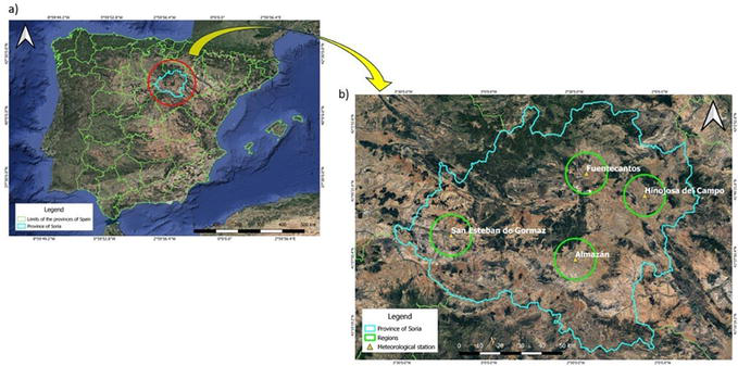
The study area includes four representative regions of the drylands cropping systems in Spain in the province of Soria (Figure 1). Each area has a size of 314.16 km², and they were built around a meteorological station that belongs to the red SiAR [41]. The four stations are located in municipalities of Almazán, Hinojosa del Campo, Fuentecantos, and San Esteban de Gormaz. These regions are characterized by a Csb climate according to Köppen-Geiger classification with hot and dry summers and cold winters [42].

Figure 1.

Study area: Location of Soria in Spain (a) and a zoom into Soria (b) with the four studied regions: Region 1: San Esteban de Gormaz, Region 2: Fuentecantos, Region 3: Hinojosa del Campo, and Region 4: Almazán.

Table 1 shows the differences between sites in terms of precipitation and temperature annual values (study period 2002–2023) and the main soils of the four regions. The mean annual temperature ranges from 9.89 to 11.11°C and annual precipitation from 1078 to 1332 mm.

Region	Name	Mean annual temperature (°C)	Annual precipitation (mm)	Soil
Region 1	San Esteban de Gormaz	11.11	1212	Fluvisol/Cambisol
Region 2	Fuentecantos	9.89	1332	Cambisol
Region 3	Hinojosa del Campo	10.70	1189	Cambisol
Region 4	Almazán	10.68	1078	Cambisol

Table 1.

Meteorological and soil data for the four studied regions.

3. Materials

3.1 Remote sensing data

The remote sensing imagery used in the study consists of 1046 eight-day MODIS composites for the tile h17v04, spanning from 18th February 2000 to 9th November 2022. Satellite images were obtained from the MODIS MOD09A1 version 6.1 surface [43] reflectance product, available through the NASA Distributed Active Archive Centre, DAAC (https://lpdaac.usgs.gov/). This product consists of seven surface reflectance bands in the visible (VIS), near-infrared (NIR), and shortwave infrared (SWIR) regions at 500 m of spatial resolution. Specifically, the bands are centered around the following wavelengths: 470 nm (blue), 555 nm (green), 645 nm (red), 858 nm (NIR), 1240 nm (SWIR1), 1640 nm (SWIR2), and 2130 nm (SWIR3).

3.2 CORINE Land Cover (CLC) 2018

CLC2018 was used to delimit rainfed arable lands in Soria province using the class with the code 211 “non-irrigated arable lands” obtaining a total surface of 455.400 hectares (18,216 pixels). This dataset offers consistent and detailed information on land cover and land cover changes across Europe, being produced in the frame of the Copernicus Land Monitoring Service and coordinated by the European Environment Agency (EEA). The minimum mapping unit is 25 hectares for status layers and 5 hectares for land cover changes [44]. It was downloaded in the shapefile format from the Spanish platform for open datasets (https://datos.gob.es/es). Polygons were rasterized to 500 meters of spatial resolution to match with MODIS imagery and used to mask the other land cover classes and remove them from the analysis.

4. Methods

4.1 NDVI time series generation

MODIS imagery was downloaded from the NASA Distributed Active Archive Centre, DAAC, and re-projected to the UTM Zone 30 N WGS84 coordinate system. NDVI values for each composite were calculated [45] (Eq. (1)):

$$\text{NDVI}=\frac{\left(NIR-\text{R}\right)}{\left(NIR+\text{R}\right)}$$E1

Where R and NIR represent pixel reflectance values in the red and near-infrared bands, respectively.

NDVI time series were generated and smoothed in order to avoid anomalous values. First, observations that fell outside the threshold of the mean plus/minus twice the standard deviation within a five-date period window were considered as outliers and replaced by the average of the previous and subsequent observations in the time series. Then, a Savitzky-Golay filter [46] was applied with a smoothing window width of 9 and a degree of the smoothing polynomial of 2 [47].

4.2 Subseting NDVI time series

The regions of interest (ROIs) were selected based on the location of four meteorological stations and delimited by intersecting circular surfaces with 10 km of radius around these stations and the non-irrigated arable lands identified with CLC 2018 dataset. As a result, a total of 2584 time series (i.e., pixels) were analyzed.

4.3 NDVI time series modeling

NDVI time series dynamics reflect vegetation conditions driven by climate and other factors resulting in a significant seasonality with an annual pattern repeated every 46 observations based on the frequency of MODIS data acquisition, which is 8 days. The presence of this seasonality is the main reason for non-stationarity in the NDVI time series.

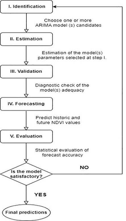
Data-driven modeling based on Statistical Time Series Analysis in the frequential and temporal domains [24, 48] has been used to model and forecast NDVI time series. The procedure has been implemented using the original NDVI time series in the following stages [24] (Figure 2):

Figure 2.

Flow chart of the Box and Jenkins methodology.

4.3.1 Identification

In this step, NDVI time series dynamics were analyzed to identify their characteristic components such as seasonality, cycles, trends, or structural changes, among others. With this information, a specific model was proposed for each series. The identification stage was made at pixel level through the following stages:

1. I.1. Preliminary statistics analysis.

2. I.2. Estimation and analysis of the autocorrelation functions (regular and partial).

3. I.3. Estimation and analysis of the periodogram and use of white noise tests such as Fisher’s Kappa (Fk) and Barlett’s Kolgomoroff–Smirnoff (BKS) tests [49] to detect significant periodic components.

4. I.4. The regular and seasonal autoregressive and moving-average parameters were specified based on the preceding identification results to capture the dynamics of each series effectively.

4.3.2 Estimation

Nonlinear least squares methods were used to estimate the models specified in the previous stage, while the Akaike and Schwarz Information Criteria were employed to select the most suitable model [48]. The Student-t and F tests were used to evaluate the significance of the model parameters.

4.3.3 Validation

The NDVI variable was predicted using the selected models in the drylands of Soria. The adequacy of the estimated models was assessed using the autocorrelation in the model residuals through the Ljung-Box Q statistic [50]. If the test reveals that a substantial amount of residual autocorrelation persists in the estimated models, the model is considered invalid, and returning to the Identification step is necessary. Q Ljung-Box test [50] estimations were done for several lags within a logical temporal horizon (92 lags), given that the NDVI temporal frequency is 46 observations per year.

4.3.4 Forecasting

Historical and future NDVI values were predicted using the validated models.

4.3.5 Prediction evaluation

To assess the predictive capacity of the models, we used Theil’s U inequality coefficient [51]. This coefficient is invariant to the measurement scale and ranges between 0 and 1. If U = 0, the prediction is perfect; if U = 1, the prediction is naïve (Eq. (2)). Theil’s U inequality coefficient helps us also to detect the source of the prediction error. It is broken down into three proportions: (1) The bias proportion (U^B), which tells us how far the mean of the prediction is from the mean of the observed series; (2) the variance ratio (U^V), which tells us how far the predicted variance is from the variance of the observed series; and (3) the proportion of covariance (U^C), which measures the remaining and unsystematic errors of prediction. The sum of the 3 proportions is equal to 1. For a good prediction, the proportions of bias and variance should be close to zero, and most of the error should be concentrated in the proportion of covariance.

$$U=\frac{{\left[{\displaystyle {\sum }_{i=1}^n{\left(F_i-O_i\right)}^2}\right]}^{1/2}}{{\left[{\displaystyle {\sum }_{i=1}^n{\left(O_i\right)}^2}\right]}^{1/2}}$$E2

Where:

U = Theil’s U inequality coefficient.

F_i = Forecasted variable.

O_i = Observed variable.

n = number of observations.

Statistical analyses were conducted using SAS 9.2, while image processing was performed using ENVI 4.7.

5. Results

5.1 Identification

The identification of the NDVI series has been carried out using the Box-Jenkins methodology in the selected 2584 pixels of Soria in which rainfed agriculture is practiced.

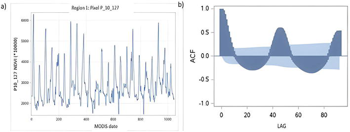
Figures 3 and 4 show one selected pixel as an example of the identification stage with the original time series, the autocorrelation functions, and the periodograms.

Figure 3.

Original time series (a) and autocorrelation function (ACF) (b) of pixel P_10_27 of Region 1: San Esteban de Gormaz.

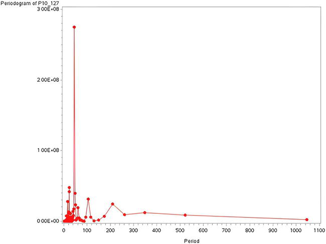
Figure 4.

Periodogram of pixel P_10_27 of Region 1: San Esteban de Gormaz.

A high temporal and spatial variability in the NDVI dynamics in these drylands has been identified, which makes it difficult to estimate models with sufficient statistical adequacy and high spatial representativeness. The analysis of the autocorrelation functions, the periodogram, and the augmented Dickey-Fuller test [52] rejected the presence of trends in most of these series.

The most common dynamic characteristic of all NDVI-studied time series was seasonality; however, this component presents a great spatial variability and a high temporal irregularity, which makes it especially difficult to incorporate it into a statistically significant and robust predictive model. In most of the time series, a dominant annual cycle was observed in period 46, with the highest ordinate, together with the presence of one or two secondary peaks of lower periodicity 23 or 14.33. Fisher’s Kappa (Fk) and Barlett’s Kolgomoroff-Smirnoff (BKS) tests [49] were used to detect significant periodic components.

It has also been detected in a high number of pixels that NDVI presents a significant conditional heteroscedasticity, which needs to be adequately treated, and, in many cases, ‘ad hoc’ in the specification and estimation of the models. To try to minimize the influence of this variance, the natural logarithm transformation has been used for all the NDVI time series to build the models.

5.2 Estimation

A great number of preliminary models were estimated, and between them, a small group of them were improved in terms of specification and estimation techniques. The final model with better statistical signification and quality and spatial representativeness (the one that adjusts correctly for a larger number of pixels) was considered to have a better performance in the study area.

A SARMA model was selected in which there were 15 autoregressive terms (AR) in the short, medium, and long term; another seasonal autoregressive term in lag 42 (SAR); 4 moving average terms in the medium term (MA); and an independent term (Table 2). All the estimated parameters show a very high statistical significance in the Student’s t-test, except in some cases in which between two and five terms were not significative. It must be highlighted that the SAR term was not significative in a lot of cases, and it was the most difficult term to adjust to all the pixels. The model reached the minimization of the information criteria of Akaike and Schwarz (AIC and SBC). An example of the SARMA model applied to pixel P2_879 of Region 2 (Fuentecantos) is shown in Table 2.

Parameter	Coefficient	Std. Error	T-test	Prob > T	Lag
MU	7.961	0.079	100.4	<0.0001	0
MA 1,1	0.096	0.041	2.33	0.020	16
MA 1,2	−0.302	0.039	−7.8	<0.0001	17
MA 1,3	0.023	0.096	0.24	0.813	42
MA 1,4	0.010	0.03	0.31	0.754	43
AR 1,1	1.649	0.029	56.59	<0.0001	1
AR 1,2	−0.609	0.051	−12.04	<0.0001	2
AR 1,3	−0.246	0.049	−4.99	<0.0001	3
AR 1,4	0.117	0.042	2.76	0.006	4
AR 1,5	0.005	0.029	0.17	0.866	6
AR 1,6	0.498	0.045	11.15	<0.0001	8
AR 1,7	−0.995	0.061	−16.41	<0.0001	9
AR 1,8	0.612	0.05	12.24	<0.0001	10
AR 1,9	−0.007	0.025	−2.84	0.005	12
AR 1,10	−0.054	0.022	−2.49	0.013	15
AR 1,11	0.043	0.016	2.75	0.006	17
AR 1,12	−0.012	0.005	−2.31	0.021	25
AR 1,13	0.035	0.006	5.77	<0.0001	44
AR 1,14	−0.018	0.006	−2.86	0.004	51
AR 1,15	0.03	0.005	5.85	<0.0001	85
AR 2,1	0.034	0.101	0.34	0.735	42

Table 2.

Selected SARMA model applied to pixel P2_879 of Region 2 (Fuentecantos).

The parameters which are not significant are shown in yellow.

5.3 Validation

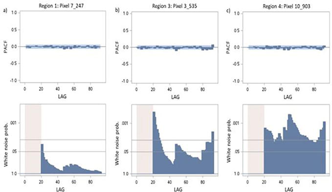
This model was implemented to the 2584 selected pixels. According to this test, pixels have been divided into three levels (Figure 5). In level 1, there were the pixels that showed low Q Ljung-Box test values at short and especially at medium and at long terms. In level three, there were the pixels that showed high Q Ljung-Box test values at short, medium, and/or long term. Therefore, the models of these pixels could be considered invalid. In level 2, there were the pixels classified as an intermediate situation; thus, the models were not invalid, but they showed higher Q Ljung-Box test values than those of level 1. Figure 5 shows the partial autocorrelation function (PACF) and white noise probability according to the Q Ljung-Box test of three selected pixels classified as level 1 (a), level 2 (b), and level 3 (c). In level 1, the PACF of the residuals was low and between the intervals of confidence. Likewise, the probability that the residuals of the models are white noise decreases as the lag order increases, being below 5% over the entire horizon. Therefore, the Q statistic is lower than the critical values of a Chi2 at 5% for all lags (except lag 20), and the null hypothesis that the residuals of the estimated model are white noise cannot be rejected. In level 3, the opposite situation could be observed.

Figure 5.

Partial autocorrelation function (PACF) and white noise probability according to the Q Ljung-Box test of three selected pixels classified as level 1 (a), level 2 (b), and level 3 (c).

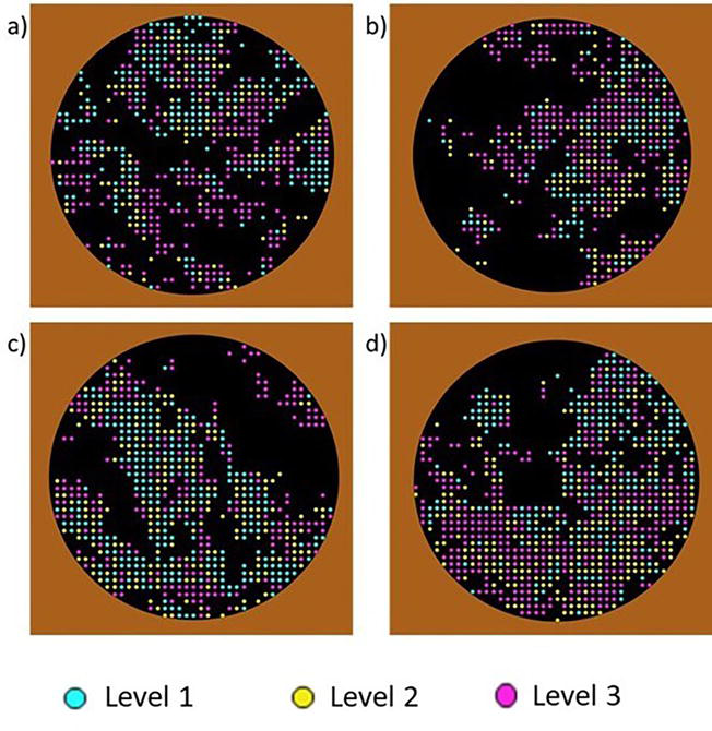
Figure 6 showed the classification and distribution of the studied pixels into the three levels according to Q Ljung-Box test:

Figure 6.

Classification and distribution into three levels of the 2584 studied pixels: (a) Region 1: San Esteban de Gormaz, (b) Region 2: Fuentecantos, (c) Region 3: Hinojosa del Campo, and d) Region 4: Almazán.

As Table 3 shows, a total of 776 pixels were classified into level 1; thus, the model showed a good adequacy for 30% of the studied pixels. The spatial distribution of the three classes showed coherence with level 2 pixels between those with level 1 and 3. Specifically, the proportion of the pixels with level 1 class is higher in regions 1 and 3 than in regions 2 and 4, with most of the pixels being in the border areas of non-irrigated arable lands.

Level	Region 1	Region 2	Region 3	Region 4	Sum	%
1	211	113	247	205	776	30.03
2	127	141	195	254	717	27.75
3	275	263	216	337	1091	42.22
Sum	613	517	658	796	2584	100

Table 3.

Number and percentage of the different pixel levels for the four selected regions.

5.4 Forecasting

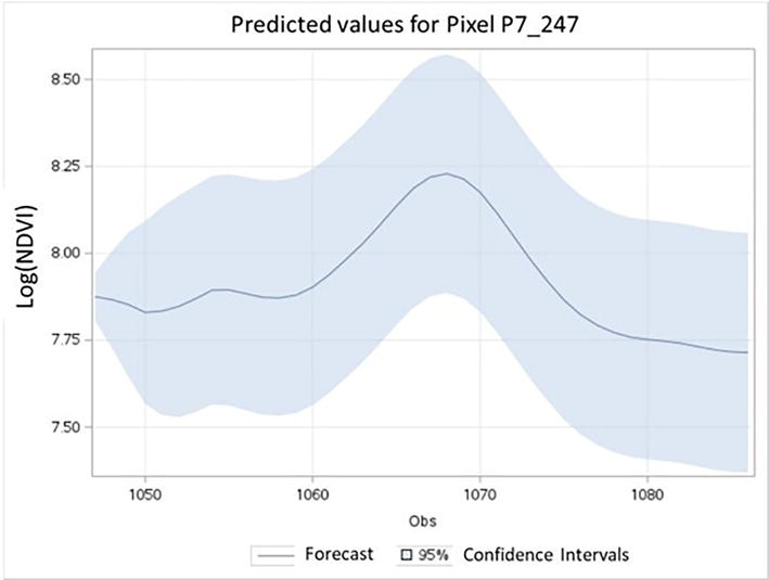
Historical values for the 1046 MODIS dates were predicted using the validated models. Future NDVI values were predicted for 46 MODIS dates (one year). Figure 7 shows the predicted 46 values for the Log(NDVI) for the pixel P7_247 of Region 1 classified as level 1. As it can be observed, the predictions were accurate, and they were inside the intervals of confidence at 95%.

Figure 7.

Predicted 46 values for the Log(NDVI) for the pixel P7_247 of Region 1 (San Esteban de Gormaz) classified as level 1.

5.5 Prediction evaluation

Table 4 shows the accuracy of the 16 model forecasts using Theil’s U inequality coefficient, which is broken down into three proportions: (1) The bias proportion (U^B), (2) the variance ratio (U^V), and (3) the proportion of covariance (U^C). As can be observed, in all cases, Theil’s U inequality coefficient was near to zero, showing a good predictive capacity of the models. In addition, most of the error was concentrated in the proportion of covariance, indicating good accuracy of the forecasts.

Region	Pixel	Level	U THEIL	U^B	U^V	U^C
1	P10_133	1	0.00516	1.49572E−05	0.00410	0.99589
	P7_247	1	0.00447	1.83618E−05	0.00427	0.99572
	P10_118	2	0.00571	2.77866E−05	0.00348	0.99649
	P11_894	2	0.00375	4.65361E−05	0.00503	0.99492
2	P2_880	1	0.00536	2.61424E-05	0.00359	0.99639
	P3_776	1	0.00529	2.23460E-05	0.00559	0.99438
	P2_936	2	0.00443	7.53839E-06	0.00278	0.99721
	P1_939	2	0.00544	1.51601E-05	0.00384	0.99614
3	P3_803	1	0.00637	2.36657E-05	0.00543	0.99454
	P3_996	1	0.01006	3.12941E-06	0.01324	0.98676
	P3_535	2	0.00590	5.99829E-05	0.00407	0.99587
	P3_536	2	0.00647	4.80825E-05	0.00569	0.99426
4	P11_826	1	0.00651	7.32773E-07	0.00474	0.99525
	P11_980	1	0.00789	3.28687E-05	0.00573	0.99423
	P11_362	2	0.00432	1.89298E-05	0.00452	0.99546
	P11_457	2	0.00393	4.48277E-05	0.01533	0.98462

Table 4.

Accuracy of the model forecasts for 16 pixels of level 1 and level 2 using the Theil’s U inequality coefficient which is broken down into three proportions: (1) The bias proportion (U^B), (2) The variance ratio (U^V), (3) The proportion of covariance (U^C).

6. Conclusions

The analysis of the NDVI time series in the studied area has revealed a high temporal and spatial variability in its dynamics. However, it has made it possible to identify several common characteristics such as the absence of a long-term trend (autocorrelation, periodogram, and stationarity tests) and a very significant annual seasonality that dominates the dynamics of most of these series.

The selected model has shown high global adequacy in the construction stage of the dynamic model, and it has shown a satisfactory performance for 30% of the studied pixels.

This study is a first step in trying to model and forecast the NDVI of rainfed crops in mainland Spain. However, further research is needed to build an appropriate model valid for more pixels. In the next step, multivariate time series analysis must be applied to build dynamic NDVI models including variables such as precipitation and temperature, which are essential in the development of rainfed crops.

Acknowledgments

We would like to thank the participation of Quasar s.l. y Prosecar s.l. in this research project. This research was conducted in the framework of the European project Forward. VC was supported by a postdoctoral Juan de la Cierva fellowship (FJC2021-046735-I) funded by the Spanish Ministerio de Ciencia e Innovación MCIN/AEI/10.13039/501100011033 and by the European Union << NextGenerationEU >>/<< PRTR >>. LR was supported by a UPM grant as part of the national research program Recualificación del Sistema Universitario Español, financed by the Recovery and Resilience Package—NextGenerationEU (European Commission). CS was also supported by a predoctoral scholarship awarded by the Community of Madrid (No. IND2020/AMB-17747).

Conflict of interest

The authors declare no conflict of interest.