The Influence of Flow Admixtures to the Electromagnetic Flow Meter Accuracy

Abstract

The measurement error appears in an electromagnetic flow meter when the flow has admixtures with magnetic and/or electric properties different from the fluid. The particle shape approximates the ellipsoid. The reasons of error appeared inside and outside of the particles in the active zone of the flow meter with any canal form and turbulent flow investigated. The investigation is performed by analogy among electrostatic, magnetic, and electric current fields. Expressions for error depending on volume concentration, permeability, electric conductivity of particles, and different ellipsoid axes lengths are presented. The expressions of the error are obtained assuming that particles are oriented in various directions concerning the flow direction. Magnetic particles with the considerable value of electric conductivity are dangerous in particular. The extra measurement error depends on particle shape in this case especially. The measurement error increases if the particle shape differs from the sphere. The complementary measurement error can exceed some hundred times the volume concentration of particles if the ratio between the longest and shortest axes of the ellipsoid exceeds 10. The error is proportional to the second power of admixtures volume concentration when particles are nonmagnetic. When admixtures are nonmagnetic and nonconductive, the measurement error does not depend on the particle’s shape.

1. Introduction

Electromagnetic flow meters (EMFM) for the measurement of ionic fluid flow in closed filled pipes are investigated in this chapter. Such meters are especially suitable in modern measuring systems, which are most often part of artificial intelligence. Their natural electrical output signal and absence of inertia allow you to create high-speed control and information systems.

The theory of the electromagnetic fluid flow meter was developed in the middle of the twentieth century. The Poisson equation describing the potential induced in the active zone of the electromagnetic flow meter, i.e., in that part of the meter where the magnetic field operates, was called by J. Shercliff [1] the main equation of the theory of electromagnetic flowmetry:

$${\nabla }^2{V}_i=div\left[\mathit{v}\times \mathit{B}\right].$$E1

This differential equation reveals the absence of measurement inertia. By solving it, we can find out how the induced potential V_i will be distributed in the active zone, if we know the distribution of the velocity of the liquid v and the magnetic flux density B in it. However, this equation is not tied to the design of the meter. In the case when the vector of the magetic flux density B, the axis of the flow meter channel, and the straight line connecting the centers of the electrodes are perpendicular to each other, the induced voltage of the electrodes is convenient to express using the expression of electrode signal U_e proposed by M. Bevir [2]:

$$U_e=-\underset{{\tau }_a}{\int }\left(\mathit{J}\left[\mathit{v}\mathbf{\times }\mathit{B}\right]\right)\mathrm{d}\tau =\underset{{\tau }_a}{\int }\left(\mathit{v}\left[\mathit{B}\mathbf{\times }\mathit{J}\right]\right)\mathrm{d}\tau ={\int }_{{\tau }_a}\mathit{vW}\mathrm{d}\tau ,$$E2

where τ_a is the volume of active zone of flow meter, J is the vector of virtual current density, coorespondingly, in any point of active zone, W is theweight vector. The virtual current density J is a formal parameter. It can be calculated as density of the current driving in the fluid at rest when to the electrodes of flow meter is connected source of current equal to 1 A [2]. Bevir proved this dependence as a theorem, so it accurately applies the basic equation of the electromagnetic flow meter to the selected design. The virtual current and weight vector are the fundamental units in theory of electromagnetic flow meters which allow to evaluate the influence of different parameters to the measurement accuracy. In [3], it is proposed to use the virtual current for the verification of the electromagnetic flow meters.

The liquid whose flow rate is measured is considered homogeneous. The theory of electromagnetic flow meters for homogeneous fluids has developed sufficiently. However, this is not always than we can suppose that liquid is homogeneous. Again the liquid may be contaminated with certain impurities or due to the leaking of the pipeline air bubbles can get into it. Therefore, it is important to find out how different admixtures change the measurement signal U_e.

With the development of the theory of electromagnetic flow meters, there were considered cases when the liquid is heterogeneous [4, 5, 6, 7, 8], but these were partial cases, usually intended at one type of heterogeneity. At Kaunas University of Technology, there were carried out systematic research to correlate the magnitude of measurement errors arising from various types of admixtures with the different physical properties and shape of those admixtures [9, 10, 11, 12]. This chapter of the book summarizes the results obtained by Department of Electrical Power Systems of Kaunas University of Technology.

2. The basic equations, admixture shapes, and coordinate systems

Eq. (2) is especially suitable for the study of the influence of various admixtures on the electrode signal U_e, because the magnetic properties of admixtures will change the distribution of the magnetic flux density, and the electrical properties will change the distribution of virtual current, so we can perform a strict quantitative analysis.

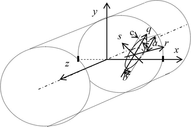
The electrode signal of the electromagnetic flow meters is formed by any point of the active zone. We joined with the active zone the global rectangular coordinate system xyz (see Figure 1). The influence of any active zone point x, y, z to the measurement signal depends on the value of the weight vector in this point $\mathit{W}\left(\mathit{x},\mathit{y},\mathit{z}\right)\mathit{=}\mathit{B}\left(\mathit{x},\mathit{y},\mathit{z}\right)\times \mathit{J}\left(\mathit{x},\mathit{y},\mathit{z}\right)$ [2].

Figure 1.

Global and local coordinate systems.

The expressions for measurement signal errors when the fluid is contaminated by small magnetic particles depending on volume concentration, permeability, and electric conductivity of particles are obtained in [9] for spherical particles and for an ideal electromagnetic flow meter with a rectangular duct and infinitely conductive large electrodes.

The real shape of particles is different from the sphere frequently. The shape of particles will change the distribution of densities of virtual current and magnetic flux when the physical properties of particles are different than fluid. Therefore, it is important to investigate the dependence of measurement error on the shape of admixture particles.

We approximate the particle shape by an ellipsoid. This shape allows generalizing the particles of very different forms. The limiting cases of ellipsoids are spheres, disks, cylinders, lamella, and others. Some different particular cases are investigated in [10, 11]. We generalize all cases for the ellipsoidal shape of particles and any form of a channel with the point electrodes. We suppose that fluid flow is parallel to z axis, i.e., flow velocity has only component v_z, z axis coincides with channel axis, and x axis coincides with the line jointed centers of electrodes. The investigation is performed for flat flow velocity distribution in the channel cross section and the mean value of velocity equal to $\overline{v}=1\mathrm{m}/\mathrm{s}$. We call this regime as normalized. Signal U can be expressed in this case [9]:

$$\left\{\begin{array}{c}U={\int }_{{\tau }_a}{W}_z\mathrm{d}\tau ,\\ W_z=J_x{B}_y-J_y{B}_x.\end{array}\right.$$E3

where τ_a–volume of the active zone; W_z = W_z(x, y, z)–z component of the weight vector in the point x, y, z of the active zone, J_x(x, y, z), B_x = B_x(x, y, z), J_y = J_y(x, y, z), B_y = B_y(x, y, z)–the x and y components of the virtual current J and magnetic flux B densities vectors in this point.

Using expression (3), we can evaluate how the magnetic and electric properties of the admixtures act to measurement error. To find the admixture influence to the electrode signal, it is needed to investigate the variation of the magnetic flux and the virtual current densities distribution in any active zone point. Evaluating that the weight vector can be different in the any active zone point we express the value of the measurement signal U₀ when the admixtures are absent in the flow as follows:

$$\left\{\begin{array}{l}{U}_0=\left(\frac{1}{{\tau }_a}\underset{{\tau }_a}{\int }{W}_{z0}d{\tau }_a\right)·{\tau }_a=\overline{W_{z0}}{\tau }_a,\\ \overline{W_{z0}}=\overline{J_{x0}{B}_{y0}}-\overline{J_{y0}{B}_{x0}},\end{array}\right.$$E4

where J_x0 = J_x0(x, y, z), J_y0 = J_y0(x, y, z), B_x0 = B_x0(x, y, z), and B_y0 = B_y0(x, y, z)–the values of the suitable components of the vectors J and B in the point x, y, z of the active zone without admixtures, ${\overline{W}}_{z0}$, $\overline{J_{x0}{B}_{y0}}$, and$\overline{J_{y0}{B}_{x0}}$ the mean values of the weight vector z component and the products of the suitable components of J and B in the clean fluid flow.

The shape of the admixture particle we approximate by an ellipsoid which orientation in respect to the global coordinate system can be any. We use the local rectangular coordinate system q, r, s whose axes coincide with the axes of the ellipsoid as it is shown in Figure 1. The equation of ellipsoid when the longest semi-axis a coincides with the q axis, the semi-axis of the middle length b coincides with the r axis and the shortest semi-axis c coincides with the s axis is:

$$\raisebox{1ex}{$q^2$}\!\left/ \!\raisebox{-1ex}{$a^2$}\right.+\raisebox{1ex}{$r^2$}\!\left/ \!\raisebox{-1ex}{$b^2$}\right.+\raisebox{1ex}{$s^2$}\!\left/ \!\raisebox{-1ex}{$c^2$}\right.=1$$E5

In this equation, a, b, and c are the lengths of the ellipsoid semi-axes. We can obtain very different forms of particles varying the ratios a/b and b/c.

In the general case, the measured flow can be turbulent or laminar. However, in the case of laminar flow, it is difficult to obtain generalizing expressions. Magnetic particles can be exposed to the magnetic field of the active zone, and they will begin to drift along the lines of the magnetic field, and that drift will depend on the flow rate. Heavier particles will be affected by the force of gravity, they will move to the bottom, and that movement will also depend on the speed of the liquid.

Therefore, we will limit further consideration to the turbulent flow. In the turbulent stream, fine particles will rotate and it can be assumed that they will not be affected by the gravity and magnetic forces.

It is very important to find out all the causes of errors, since they are also relevant when using an electromagnetic flow meter for measuring two-phase and three-phase flows.

In [9], four different components of signal error are indicated when some admixture particles get into active zone of the flow meter. The first component emerges due to the variation of virtual current and (or) magnetic flux density in the volume which the particles occupied. The other components arise for the variation of virtual current and magnetic flux density in the volume outside the particles. We can divide three different error components arising outside the admixture particles: because of the distortion of the virtual current and the magnetic flux density lines (supposing that its magnitudes were not varied), because of the variation of the magnetic flux density magnitude and because of the variation of the virtual current magnitude. Let’s evaluate these.

3. The component of the signal error inside the admixture particle

The mean value of the weight function inside the ellipsoidal particle we can express this way:

$${\overline{W}}_{z\mathrm{p}}=\overline{J_{x\mathrm{p}}{B}_{y\mathrm{p}}}-\overline{J_{y\mathrm{p}}{B}_{x\mathrm{p}}}=K_F^I\overline{J_{x0}{B}_{y0}}-K_F^{\mathit{II}}\overline{J_{y0}{B}_{x0}}.$$(6)E6

We suppose that particles are small and distributed evenly in the flow. The components J_x = J_x (x, y, z), J_y = J_y (x, y, z), B_x = B_x (x, y, z), and B_y = B_y(x, y, z) are not varied strictly by varying x, y, z. For small particles, we can suppose that independently on the meter design the components J_x = J_x (x, y, z), J_y = J_y (x, y, z), B_x = B_x (x, y, z), and B_y = B_y(x, y, z) have the same value in all volume which particle occupies before the particle gets into the flow, i.e., they are distributed uniformly. Therefore, in the ellipsoidal particle volume, they will be distributed uniformly too (see [13]).

We will study the distribution of the magnetic field of the electrostatic field in the dielectric ellipsoid, presented in [13], and the analogy of the electrostatic, magnetic, and electrical current fields.

Suppose that before the dielectric ellipsoid gets in field, there was a homogeneous electrostatic field E, the components of which in the local coordinate system directed by the semi-axes of ellipsoid, a, b, and c were E_a0, E_b0, and E_c0. Inside the dielectric ellipsoid, the components by [13] will be

$$E_{\mathit{ap}}=\frac{C_a{\epsilon }_f{E}_{a0}}{\left(C_a-1\right){\epsilon }_f+{\epsilon }_p},E_{\mathit{bp}}=\frac{C_b{\epsilon }_f{E}_{b0}}{\left(C_b-1\right){\epsilon }_f+{\epsilon }_p},E_{\mathit{cp}}=\frac{C_c{\epsilon }_f{E}_{c0}}{\left(C_c-1\right){\epsilon }_f+{\epsilon }_p},$$E7

where ε_p is the relative permittivity of the ellipsoid and ε_f is the relative permittivity of the environment, C_a, C_b, and C_c are the ellipsoid shape factors expressed in [13] as follows:

$$\left\{\begin{array}{c}{\mathit{C}}_{\mathit{a}}=\frac{\mathbf{2}}{\mathit{abc}{\int }_{\mathbf{0}}^{\infty }\raisebox{1ex}{$\mathbf{d}\mathit{w}$}\!\left/ \!\raisebox{-1ex}{$\sqrt{{\left(\mathit{w}+{\mathit{a}}^{\mathbf{2}}\right)}^{\mathbf{3}}\left(\mathit{w}+{\mathit{b}}^{\mathbf{2}}\right)\left(\mathit{w}+{\mathit{c}}^{\mathbf{2}}\right)}$}\right.},\\ {\mathit{C}}_{\mathit{b}}=\frac{\mathbf{2}}{\mathit{abc}{\int }_{\mathbf{0}}^{\infty }\raisebox{1ex}{$\mathbf{d}\mathit{w}$}\!\left/ \!\raisebox{-1ex}{$\sqrt{\left(\mathit{w}+{\mathit{a}}^{\mathbf{2}}\right){\left(\mathit{w}+{\mathit{b}}^{\mathbf{2}}\right)}^{\mathbf{3}}\left(\mathit{w}+{\mathit{c}}^{\mathbf{2}}\right)}$}\right.}\\ {\mathit{C}}_{\mathit{b}}=\frac{\mathbf{2}}{\mathit{abc}{\int }_{\mathbf{0}}^{\infty }\raisebox{1ex}{$\mathbf{d}\mathit{w}$}\!\left/ \!\raisebox{-1ex}{$\sqrt{\left(\mathit{w}+{\mathit{a}}^{\mathbf{2}}\right)\left(\mathit{w}+{\mathit{b}}^{\mathbf{2}}\right){\left(\mathit{w}+{\mathit{c}}^{\mathbf{2}}\right)}^{\mathbf{3}}}$}\right.}.\end{array}\right.,$$E8

By the fields analogy in the field of the electric current, the vector J of the current density and in the magnetic field the vector B of the magnetic flux density correspond to displacement vector D in the electrostatic field. Evaluating relation between the vectors E and D we can interconnect the components of vector D_p inside the ellipsoid D_ap, D_bp, and D_cp with the vector D₀ components D_a0, D_b0, and D_c0 before the ellipsoid gets into the field this way:

$$\begin{array}{l}{D}_{\mathit{ap}}={\epsilon }_p{\epsilon }_0{E}_{\mathit{ap}}=\frac{{\epsilon }_p{C}_a{\epsilon }_f{\epsilon }_0{E}_{a0}}{\left(C_a-1\right){\epsilon }_f+{\epsilon }_p}=\frac{{\epsilon }_p{C}_a}{\left(C_a-1\right){\epsilon }_f+{\epsilon }_p}{D}_{a0}=\frac{C_a}{\left(C_a-1\right)\raisebox{1ex}{${\epsilon }_f$}\!\left/ \!\raisebox{-1ex}{${\epsilon }_p$}\right.+1}{D}_{a0}\\ =A_a^{\epsilon }{D}_{a0},\\ D_{\mathit{bp}}=\frac{C_b}{\left(C_b-1\right)\raisebox{1ex}{${\epsilon }_f$}\!\left/ \!\raisebox{-1ex}{${\epsilon }_p$}\right.+1}{D}_{\mathit{bp}}=A_b^{\epsilon }{D}_{b0},\\ D_{\mathit{cp}}=\frac{C_c}{\left(C_c-1\right)\raisebox{1ex}{${\epsilon }_f$}\!\left/ \!\raisebox{-1ex}{${\epsilon }_p$}\right.+1}{D}_{c0}=A_c^{\epsilon }{D}_{c0},\end{array}$$E9

where ε₀ is absolute permittivity of vacuum, and $A_a^{\epsilon },A_b^{\epsilon },A_c^{\epsilon }$ are the components of matrix factor $A^{\epsilon }$which relates vectors D_p and D₀ . There is convenient to describe the components of $A^{\epsilon }$ this way:

$$A_a^{\epsilon }=1+\left(C_a-1\right){\mathrm{\kappa }}_a^{\mathrm{\epsilon }},A_b^{\epsilon }=1+\left(C_b-1\right){\mathrm{\kappa }}_b^{\mathrm{\epsilon }},A_c^{\epsilon }=1+\left(C_c-1\right){\mathrm{\kappa }}_c^{\mathrm{\epsilon }},$$E10

where ${\kappa }_a^{\gamma },{\kappa }_b^{\gamma },{\kappa }_c^{\gamma }$ are the factors of the electrostatic properties:

$${\kappa }_a^{\gamma }=\frac{1-\left({\epsilon }_f/{\epsilon }_p\right)}{1+\left(C_a-1\right)\left({\epsilon }_f/{\epsilon }_p\right)},{\kappa }_b^{\gamma }=\frac{1-\left({\epsilon }_f/{\epsilon }_p\right)}{1+\left(C_b-1\right)\left({\epsilon }_f/{\epsilon }_p\right)},{\kappa }_c^{\gamma }=\frac{1-\left({\epsilon }_f/{\epsilon }_p\right)}{1+\left(C_c-1\right)\left({\epsilon }_f/{\epsilon }_p\right)}.$$E11

The relation between the displacement vectors D_p inside the ellipsoid and D₀ outside the ellipsoid is linear. In the global coordinate system, it is

$${\left[D_{\mathit{xp}},D_{\mathit{yp}},D_{\mathit{zp}}\right]}^T=\left[h\right]\left[A^{\epsilon }\right]{\left[h\right]}^T{\left[D_{x0},D_{y0},D_{z0}\right]}^T\mathbf{.}$$E12

If the local coordinate system is turned about the x axis of global system by an angle ψ, about the y axis by an angle ν, and about the z axis by an angle φ, the elements of the matrix [h] in the expression (12) is [14]

$$\left\{\begin{array}{c}{h}_{11}=cos\nu cos\phi ,h_{12}=-sin\phi cos\nu ,h_{13}=sin\nu ,\\ h_{21}=cos\psi sin\phi +sin\psi sin\nu cos\phi ,h_{22}=cos\psi cos\phi -sin\psi sin\nu sin\phi ,h_{23}=-sin\psi cos\phi ,\\ h_{31}=sin\psi sin\phi -cos\psi sin\nu cos\phi ,h_{32}=sin\psi cos\phi +cos\psi sin\nu sin\phi ,h_{33}=cos\psi cos\nu .\end{array}\right.$$E13

By fields analogy the relations in the global coordinate system among the components of the virtual current and magnetic flux densities inside the particle J_xp, J_yp, J_zp, B_xp, B_yp, and B_zp and the suitable components before the particle get into fluid J_x0, J_y0, J_z0, B_x0, B_y0, and B_z0, we can express analogically to Eq. (12):

$${\left[J_{\mathit{xp}},J_{\mathit{yp}},J_{\mathit{zp}}\right]}^T=\left[h\right]\left[A^{\gamma }\right]{\left[h\right]}^T{\left[J_{x0},J_{y0},J_{z0}\right]}^T,$$E14

$${\left[B_{\mathit{xp}},B_{\mathit{yp}},B_{\mathit{zp}}\right]}^T=\left[h\right]\left[A^{\mu }\right]{\left[h\right]}^T{\left[B_{x0},B_{y0},B_{z0}\right]}^T$$E15

In Eq. (14), [A^γ] is a matrix factor of the electric properties of the admixtures. We express [A^γ] supposing that the axes of the ellipsoidal particle are oriented by the axes of the local coordinate system but this orientation can be any:

$$\left[A^{\gamma }\right]=\left[\begin{array}{ccc}{A}_i^{\gamma }& 0& 0\\ 0& A_j^{\gamma }& 0\\ 0& 0& A_k^{\gamma }\end{array}\right],$$E16

where

$$A_i^{\gamma }=1+\left(C_i-1\right){\mathrm{\kappa }}_i^{\mathrm{\gamma }},A_j^{\gamma }=1+\left(C_j-1\right){\mathrm{\kappa }}_j^{\mathrm{\gamma }},A_k^{\gamma }=1+\left(C_k-1\right){\mathrm{\kappa }}_k^{\mathrm{\gamma }},$$E17

$$\begin{array}{c}{\kappa }_i^{\gamma }=\frac{1-\left({\gamma }_f/{\gamma }_p\right)}{1+\left(C_i-1\right)\left({\gamma }_f/{\gamma }_p\right)},\\ {\kappa }_j^{\gamma }=\frac{1-\left({\gamma }_f/{\gamma }_p\right)}{1+\left(C_j-1\right)\left({\gamma }_f/{\gamma }_p\right)},{\kappa }_k^{\gamma }=\frac{1-\left({\gamma }_f/{\gamma }_p\right)}{1+\left(C_k-1\right)\left({\gamma }_f/{\gamma }_p\right)}.\end{array}$$E18

In Eqs. (16)–(18), $i=a\text{or}b\text{or}c;j=a\text{or}b\text{or}c$; $k=a\text{or}b\text{or}c,$ $i\ne j\ne k.$ Electric properties of the admixtures and the fluid in case of the electric current are expressed by γ_p and γ_f–electric conductivities of particles and fluid, accordingly. The ${\kappa }_i^{\gamma },$ ${\kappa }_j^{\gamma },\text{and}{\kappa }_k^{\gamma }$ are the factors of the electric conductivity.

[A^μ] in Eq. (15) is a matrix factor of the magnetic properties of the admixtures. When the ellipsoid axes are oriented by the axes of the local coordinate system randomly, it can be expressed as follows:

$$\left[A^{\mu }\right]=\left[\begin{array}{ccc}{A}_i^{\mu }& 0& 0\\ 0& A_j^{\mu }& 0\\ 0& 0& A_k^{\mu }\end{array}\right],$$E19

$$A_i^{\mu }=1+\left(C_i-1\right){\mathrm{\kappa }}_{\mathrm{i}}^{\mathrm{\mu }},A_j^{\mu }=1+\left(C_j-1\right){\mathrm{\kappa }}_{\mathrm{j}}^{\mathrm{\mu }},A_k^{\mu }=1+\left(C_k-1\right){\mathrm{\kappa }}_{\mathrm{k}}^{\mathrm{\mu }},$$E20

where

$${\kappa }_i^{\mathit{\mu }}=\frac{1-\left(1/{\mathit{\mu }}_p\right)}{1+\left(C_i-1\right)\left(1/{\mathit{\mu }}_p\right)},{\kappa }_j^{\mathit{\mu }}=\frac{1-\left(1/{\mathit{\mu }}_p\right)}{1+\left(C_j-1\right)\left(1/{\mathit{\mu }}_p\right)},{\kappa }_k^{\mathit{\mu }}=\frac{1-\left(1/{\mathit{\mu }}_p\right)}{1+\left(C_k-1\right)\left(1/{\mathit{\mu }}_p\right)},$$E21

where μ_p is the permeability of particles, and ${\kappa }_i^{\mu },{\kappa }_j^{\mu },\text{and}{\kappa }_k^{\mu }$ are the factors of the permeability.

Relating the biggest semi-axis a of the ellipsoid with any of the axes of the local coordinate system and the other two semi-axes b and c with any of the remaining axes, we obtain all six possible positions of the ellipsoid in the local coordinate system. In Eqs. (10)–(15), it can be six possible combinations of i, j, k:

$$\left\{\begin{array}{c}i=a,j=b,k=c,\\ i=a,j=c,k=b,\\ i=b,j=a,k=c,\\ i=b,j=c,k=a,\\ i=c,j=a,k=b,\\ i=c,j=b,k=a.\end{array}\right.$$E22

By Eqs. (13), (16), and (19), we can express the components $J_{\mathit{xp}},J_{\mathit{yp}},B_{\mathit{xp}}$, and $B_{\mathit{yp}}$:

$$J_{\mathit{xp}}=\left(h_{11}^2{A}_i^{\gamma }+h_{12}^2{A}_j^{\gamma }+h_{13}^2{A}_k^{\gamma }\right)J_{x0}+\left(h_{11}{h}_{21}{A}_i^{\gamma }+h_{12}{h}_{22}{A}_j^{\gamma }+h_{13}{h}_{23}{A}_k^{\gamma }\right)J_{y0},$$E23

$$J_{\mathit{yp}}=\left(h_{11}{h}_{21}{A}_i^{\gamma }+h_{12}{h}_{22}{A}_j^{\gamma }+h_{13}{h}_{23}{A}_k^{\gamma }\right)J_{x0}+\left(h_{21}^2{A}_i^{\gamma }+h_{22}^2{A}_j^{\gamma }+h_{23}^2{A}_i^{\gamma }\right)J_{y0}$$E24

$$B_{\mathit{xp}}=\left(h_{11}^2{A}_i^{\mu }+h_{12}^2{A}_j^{\mu }+h_{13}^2{A}_k^{\mu }\right)B_{x0}+\left(h_{11}{h}_{21}{A}_i^{\mu }+h_{12}{h}_{22}{A}_j^{\mu }+h_{13}{h}_{23}{A}_k^{\mu }\right)B_{y0},$$E25

$$B_{\mathit{yp}}=\left(h_{11}{h}_{21}{A}_i^{\mu }+h_{12}{h}_{22}{A}_j^{\mu }+h_{13}{h}_{23}{A}_k^{\mu }\right)B_{x0}+\left(h_{21}^2{A}_i^{\mu }+h_{22}^2{A}_j^{\mu }+h_{23}^2{A}_k^{\mu }\right)B_{y0}$$E26

We will calculate the average values of the elements of Eq. (6) in two stages. In the first stage, we suppose that the local coordinate axes turned with respect to the global coordinate axes by angles φ, ψ, and ν, and semi-axes of the ellipsoid coincide with the local coordinate axes, but the axes of the local coordinate system and the ellipsoid semi-axes can be any of six possible combinations Eq. (22). The factors K_F^I and K_F^II we obtain substituting in Eq. (6) $J_{\mathit{xp}},J_{\mathit{yp}},B_{\mathit{xp}}$, and $B_{\mathit{yp}}$ expressed by Eqs. (23)–(26) for any of i, j, k combinations Eq. (16) and evaluating that the products of the collinear components J_xB_x, J_yB_y, $A_i^{\gamma }{A}_i^{\mu },A_j^{\gamma }{A}_j^{\mu },A_k^{\gamma }{A}_k^{\mu }$are equal to zero. By this we can write

$$\begin{array}{rcl}{K}_F\left(\phi ,\nu ,\psi \right)& =& \overline{K_F^I\left(\phi ,\nu ,\psi \right)}=\overline{K_F^{\mathit{II}}\left(\phi ,\nu ,\psi \right)}\\ & =& \overline{H\left(\phi ,\nu ,\psi \right)}\left(A_a^{\gamma }{A}_b^{\mathit{\mu }}+A_a^{\gamma }{A}_c^{\mathit{\mu }}+A_b^{\gamma }{A}_a^{\mathit{\mu }}+A_b^{\gamma }{A}_c^{\mathit{\mu }}+A_c^{\gamma }{A}_a^{\mathit{\mu }}+A_c^{\gamma }{A}_b^{\mathit{\mu }}\right)·\frac{1}{6}\\ & =& \overline{H\left(\phi ,\nu ,\psi \right)}·\overline{A^{\gamma }{A}^{\mathit{\mu }}},\end{array}$$E27

where

$$\begin{array}{rcl}\overline{H\left(\phi ,\nu ,\psi \right)}& =& {\left(h_{11}{h}_{22}-h_{21}{h}_{12}\right)}^2+{\left(h_{11}{h}_{23}-h_{21}{h}_{13}\right)}^2+{\left(h_{12}{h}_{23}-h_{22}{h}_{13}\right)}^2\\ & =& [{h_{11}}^2\left({h_{22}}^2+{h_{23}}^2\right)+{h_{12}}^2\left({h_{21}}^2+{h_{23}}^2\right)+{h_{13}}^2({h_{21}}^2+{h_{22}}^2)\\ & & -2(h_{11}{h}_{22}{h}_{12}{h}_{21}+h_{11}{h}_{23}{h}_{13}{h}_{21}+h_{12}{h}_{23}{h}_{13}{h}_{22})].\end{array}$$E28

We calculate the factors $A_a^{\gamma }$, $A_b^{\gamma }$, $A_c^{\gamma }$,$A_a^{\mu }$,$A_b^{\mu }$, and $A_c^{\mu }$ by Eqs. (16)–(18) and Eqs. (19)–(21) substituting i = a, j = b and k = c. For the spinning ellipsoidal particle, we calculate the mean value $\overline{\overline{H(\phi ,\upsilon ,\psi }}$) of the $\overline{H\left(\phi ,\upsilon ,\psi \right)}$ when any of the angles φ, ν, ψ vary in the interval [0, π/2]. Integrating Eq. (28) we obtain

$$\overline{\overline{H\left(\varphi ,\nu ,\psi \right)}}=\frac{8}{{\pi }^3}\underset{0}{\overset{\raisebox{1ex}{$\pi $}\!\left/ \!\raisebox{-1ex}{$2$}\right.}{\int }}\underset{0}{\overset{\raisebox{1ex}{$\pi $}\!\left/ \!\raisebox{-1ex}{$2$}\right.}{\int }}\underset{0}{\overset{\raisebox{1ex}{$\pi $}\!\left/ \!\raisebox{-1ex}{$2$}\right.}{\int }}\overline{H\left(\varphi ,\nu ,\psi \right)}\mathrm{d}\psi \mathrm{d}\varphi \mathrm{d}\nu =1.$$E29

We express the mean values of coefficients $\stackrel{=}{K_F^I}=\stackrel{=}{K_F^{\mathit{II}}}=\stackrel{=}{K_F}$ when the angles φ, ν, and ψ vary in the intervals [0, π/2] by substituting the $\overline{\overline{H\left(\phi ,\gamma ,\psi \right)}}$ instead of $\overline{H\left(\phi ,\gamma ,\psi \right)}$ in Eq. (27):

$${\overline{\overline{K}}}_F={\overline{\overline{K}}}_F^I={\overline{\overline{K}}}_F^{\mathit{II}}=\frac{1}{6}\left(A_a^{\gamma }{A}_b^{\mu }+A_a^{\gamma }{A}_b^{\mu }+A_b^{\gamma }{A}_a^{\mu }+A_b^{\gamma }{A}_c^{\mu }+A_c^{\gamma }{A}_a^{\mu }+A_c^{\gamma }{A}_b^{\mu }\right)=\overline{A^{\gamma }{A}^{\mu }}.$$E30

We can express the component of the error δ_p caused by the signal variation inside the spinning particle using Eqs. (4), (6), and (30):

$${\delta }_p=\frac{\overline{U_p}-\overline{U_0}}{\overline{U_0}}=\frac{⌈\left(\raisebox{1ex}{$1$}\!\left/ \!\raisebox{-1ex}{${\tau }_p$}\right.\right){\int }_{{\tau }_p}\left(W_{\mathit{zp}}-W_{z0}\right)d{\tau }_p⌉{\tau }_p}{⌈\left(\raisebox{1ex}{$1$}\!\left/ \!\raisebox{-1ex}{${\tau }_a$}\right.\right){\int }_{{\tau }_a}{W}_{z0}d{\tau }_a⌉{\tau }_a}=\frac{\left({\overline{W}}_{\mathit{zp}}-{\overline{W}}_{z0}\right){\tau }_p}{{\overline{W}}_{z0}{\tau }_a}=\left(\overline{\overline{K_F}}-1\right)k=\left(\overline{A^{\gamma }}\overline{A^{\mu }}-1\right)k,$$E31

where τ_p is the volume of the particle and

$$k={\tau }_p/{\tau }_a$$E32

is the volume concentration of admixtures. $\overline{A^{\gamma }{A}^{\mu }}$ is expressed by Eq. (30).

Eq. (30) is the same for any ellipsoidal particle. It can be generalized for all admixture particles. In this case, τ_p is the volume of all admixture particles.

Substituting Eqs. (17) and (20) into Eq. (31), we can express the error arising inside the admixture particles as follows:

$${\delta }_p=\begin{array}{l}\frac{1}{6}k\{2\left[\left(C_a-1\right)\left({\kappa }_a^{\gamma }+{\kappa }_a^{\mu }\right)+\left(C_b-1\right)\left({\kappa }_b^{\gamma }+{\kappa }_b^{\mu }\right)+\left(C_c-1\right)\left({\kappa }_c^{\gamma }+{\kappa }_c^{\mu }\right)\right]\\ +\left(C_a-1\right)\left(C_b-1\right)\left({\kappa }_a^{\gamma }{\kappa }_b^{\mu }+{\kappa }_b^{\gamma }{\kappa }_a^{\mu }\right)+\left(C_a-1\right)\left(C_c-1\right)\left({\kappa }_a^{\gamma }{\kappa }_c^{\mu }+{\kappa }_c^{\gamma }{\kappa }_a^{\mu }\right)\\ +\left(C_b-1\right)\left(C_c-1\right)\left({\kappa }_b^{\gamma }{\kappa }_c^{\mu }+{\kappa }_c^{\gamma }{\kappa }_b^{\mu }\right)\}.\end{array}$$E33

4. The error component because of virtual current and magnetic field distortion outside particles

When a particle with volume τ_p and properties different from the fluid physical properties gets into the active zone, it distorts the magnetic field and the virtual current in the residual active zone volume τ_a-τ_p. The variation of the electrode signal ΔU_d because of this distortion will be

$$∆U_d=\underset{{\tau }_a-{\tau }_p}{\int }\overline{∆W_{z\left(-\mathrm{p}\right)}}\mathrm{d}\tau ,\overline{∆W_{z\left(-\mathrm{p}\right)}}=\overline{W_{z\left(-\mathrm{p}\right)}}-\overline{W_{z0}},$$E34

where $\overline{W_{z\left(-\mathrm{p}\right)}}$ are the mean value of the weight vector z component in the any point of volume τ_a-τ_p outside the particle.

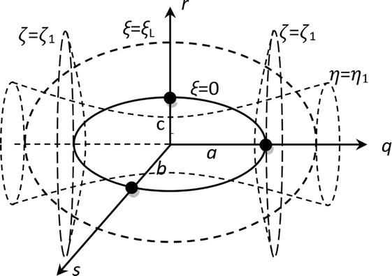
We use for ΔU_d investigation the local ellipsoidal coordinate system ξ, η, ζ [13]. The link of this system with the local rectangular coordinate system q, r, s is shown in Figure 2.

Figure 2.

The rectangular q, r, s and ellipsoidal ξ, η, ζ local coordinate systems.

The coordinate ξ = const is the same on the surface of some ellipsoid, the coordinate η = const is the same on the surface of a hyperboloid with axis q, and the coordinate ζ = const is the same on the two parallel surfaces of a hyperboloid with axis s.

Suppose that equation of the ellipsoidal particle surface is ξ = 0 in the ellipsoidal coordinate system. To calculate the function$\overline{\mathrm{\Delta }{W}_z}\left(\xi \right)$, we use the Green’s theorem written as follows:

$${\int }_{\tau -{\tau }_p}\left(grad\psi grad\phi \right)\mathrm{d}\tau =\underset{S}{\oint }\psi \left(grad\phi \mathbf{d}\mathit{S}\right)-\underset{\tau -{\tau }_p}{\int }\psi \text{divgrad}\phi \mathrm{d}\tau .$$E35

Let $grad\phi ={\mathit{e}}_{\mathit{\xi }}\overline{∆W_z\left(\xi \right)}$ and $\psi =\int h_{\xi }\mathit{d\xi }$ (h_ξ is Lame coefficient of coordinate ξ in the ellipsoidal coordinate system). Then $\frac{\partial \psi }{\partial \xi }=h_{\xi }$ and $grad\psi ={\mathit{e}}_{\mathit{\xi }}\frac{1}{h_{\xi }}\frac{\partial \psi }{\partial \xi }={\mathit{e}}_{\mathit{\xi }}\mathit{.}$ Surface S in the second integral of Eq. (35) is composed of the surfaces ξ = 0 and ξ = ξ_L > 0. We can write $\text{divgrad}\phi =div\left({\mathit{e}}_{\mathit{\xi }}\overline{∆W_z}\right)=0$ because in the volume τ_a-τ_p there are not the sources of J and B. Therefore, we can express the electrode signal variation ΔU_d due to the virtual current and the magnetic field distortion this way:

$$∆U_d=\underset{\tau -{\tau }_p}{\int }\overline{∆W_z\left(\xi \right)}\mathrm{d}\tau =\underset{S}{\oint }{\left[h_{\xi }\mathrm{d}\xi \right]}_S\overline{∆W_z\left(\xi \right)}\mathrm{d}S=I_{\xi =0}+I_{\xi ={\xi }_L};$$E36

where I_ξ = 0 and I_ξ = ξL are the values of the surface integral on the ellipsoidal particle surface and on the surface ξ_L = const, correspondingly.

Let us investigate the particle with γ_p → ∞ and μ_p → ∞. On the surface ξ = 0 of such particle, it is right equality $\overline{W_{z\infty }}={\left(\mathit{J}\mathit{\times }\mathit{B}\right)}_{\mathrm{\xi }=0}=0$ because both vectors J and B are perpendicular to the surface at any surface point. Its directions coincide, and the vector product [J × B] is equal to zero. This equality is independent on the particle position with respect to the global coordinate system.

By this equality, we can express the mean value of the variation ${\overline{\mathrm{\Delta }W}}_{z\infty }\left(0\right)$ of the weight vector z component on the surface of the particle with γ_p → ∞ and μ_p → ∞:

$${\overline{\mathrm{\Delta }W}}_{z\infty }\left(0\right)=\overline{W_{z\infty }}-{\overline{W}}_0=-{\overline{W}}_0=-\left(\overline{J_{x0}{B}_{y0}}-\overline{J_{y0}{B}_{x0}}\right).$$E37

Because $\overline{∆W_{z\infty }}=-W_0$ does not depend on the ellipsoidal coordinates ξ, η, and η, the integral I_ξ = 0 we can write as product of $-W_0$ and integral which expresses the particle volume:

$$\begin{array}{rcl}\Delta U_d& =& I_{\xi =0}=\underset{S_{\xi =0}}{\int }{\left[\int h_{\xi }\mathrm{d}\xi \right]}_{\xi =0}\overline{∆W_{z\infty }}\left(0\right)\mathrm{d}S+I_{\mathrm{\xi L}}\\ & =& -W_0{\int }_{-b^2}^{-c^2}{\int }_{-a^2}^{-b^2}{\left[h_{\xi }\mathrm{d}\xi \right]}_{\xi =0}\left(h_{\eta }{h}_{\varsigma }\right)\mathrm{d}\eta \mathrm{d}\varsigma =-W_0{\tau }_p+I_{\mathrm{\xi L}},\end{array}$$E38

where h_η and h_ζ are Lame coefficients of the coordinates η and ζ in the ellipsoidal coordinate system.

With the increase of the coordinate ξ_L > 0, the shape of ellipsoid ξ = ξ_L is neared to the shape of sphere with the radius $R=\sqrt{\xi +a^2}$(see [13]) and integral I_ξ = ξL can be expressed in the spherical coordinates. With R increase, I_ξL very quickly decreases to zero: I_ξL = (−W₀τ_p)(a³/R³) → 0. Therefore, outside the particle with γ_p → ∞ and μ_p → ∞, the signal variation by Eqs. (30) and (32) is

$$∆U_{d\infty }=-\overline{W_0}{\tau }_p$$E39

This result can be obtained other way. When γ_p → ∞ and μ_p → ∞, the electric resistance for J and the magnetic resistance for B are equal to zero and the densities of virtual current and magnetic flux cannot exchange in the particle volume τ_p. Therefore, the vector product [J × B] will be equal to zero not only on surface but also in all particle volume. The ${\overline{W}}_0$will be the same in all volume of clean fluid and in the volume outside a particle with γ_p → ∞ and μ_p → ∞. By this, we can write

$$∆U_{d\infty }={\int }_{{\tau }_{a-{\tau }_p}}{\overline{W}}_0\mathrm{d}\tau -{\int }_{{\tau }_a}{\overline{W}}_0\mathrm{d}\tau ={\overline{W}}_0{\tau }_a-{\overline{W}}_0{\tau }_p-{\overline{W}}_0{\tau }_a=-{\overline{W}}_0{\tau }_p.$$E40

In [9], it was presented such expression for the signal deviation because the magnetic field and the virtual current distortion $∆U_d=-{\kappa }^{\gamma }{\kappa }^{\mu }{W}_0{\tau }_p.$Evaluating that ${\kappa }^{\gamma }=1\text{when}\mathrm{\gamma }\to \infty$ and ${\kappa }^{\mu }=1,\text{when}\mathrm{\mu }\to \infty ,$ we can write $∆U_d={\kappa }^{\gamma }{\kappa }^{\mu }∆U_{d\infty }.$ This relation is suited for ellipsoidal particles too, but instead the product ${\kappa }^{\gamma }{\kappa }^{\mu }$ we must use the mean value of this product $\overline{{\kappa }^{\gamma }{\kappa }^{\mu }}$. The mean value we obtain remembering that relation between the global and the local coordinate axes can be any. Because factors$\overline{{\kappa }^{\gamma }}$and $\overline{{\kappa }^{\mu }}$are related with perpendicular one to other components$\overline{{\mathit{\Delta J}}_{x\left(y\right)}}$ and $\overline{{\mathit{\Delta B}}_{y\left(x\right)}}$, we obtain the mean value of product $\overline{{\kappa }^{\gamma }{\kappa }^{\mu }}$ multiplying only the factors ${\kappa }_{i,j,k}^{\gamma }$ and ${\kappa }_{i,j,k}^{\mu }$ related with the different ellipsoid axes. As a result, we have

$$\overline{{\kappa }^{\gamma }{\kappa }^{\mu }}=\raisebox{1ex}{$1$}\!\left/ \!\raisebox{-1ex}{$6$}\right.\left({\kappa }_a^{\gamma }{\kappa }_b^{\mu }+{\kappa }_a^{\gamma }{\kappa }_c^{\mu }+{\kappa }_b^{\gamma }{\kappa }_a^{\mu }+{\kappa }_b^{\gamma }{\kappa }_c^{\mu }+{\kappa }_c^{\gamma }{\kappa }_a^{\mu }+{\kappa }_c^{\gamma }{\kappa }_b^{\mu }\right).$$E41

Therefore, in the general case, the mean value of the signal variation $\overline{∆U_d}$, due to the virtual current and the magnetic flux distortion outside the particles, will be

$$\overline{∆U_d}=-\overline{{\kappa }^{\gamma }{\kappa }^{\mu }}{W}_0{\tau }_p.$$E42

We obtain the error δ_d because of the virtual current and the magnetic flux distortion outside the particles as the ratio between signal variation $\overline{∆U_d}$ outside particle and signal induced in volume τ_a-τ_p before the particle gets in active zone:

$${\delta }_d=\frac{\overline{∆U_d}}{\underset{{\tau }_a-{\tau }_p}{\int }\overline{W_0}\mathrm{d}\tau }=-\overline{{\kappa }^{\gamma }{\kappa }^{\mu }}\frac{\overline{W_0}{\tau }_p}{\overline{W_0}\left({\tau }_a-{\tau }_p\right)}=-\overline{{\kappa }^{\gamma }{\kappa }^{\mu }}\frac{k}{1-k}$$E43

The relation $\left|\overline{{\kappa }^{\gamma }{\kappa }^{\mu }}\right|\le 1$ is right for any values of γ and μ, so the error because of distortion of the virtual current and the magnetic field practically will not exceed the particle concentration $\left|{\delta }_d\right|\le k/\left(1-k\right)$. For nonmagnetic particles and for particles with γ_p = γ_f ${\delta }_d$ = 0.

5. The partial error caused by a deviation of mean value of magnetic flux density outside particle

We consider that at the time of measurement, the excitation current of the magnetic field is the same, I_M = const. Therefore, the magnetic field strength H₀ = const will also be the same. If there are no admixtures or they are nonmagnetic, then the magnetic flux density will be expressed by equation B₀ = μ₀H₀. Let’s consider how magnetic flux density B_y will change if a magnetic elliptical particle enters the active zone. If magnetic particles get into the active zone of the electromagnetic flow meter, the mean value of permeability μ_m varies. Expression of μ_m was obtained for the spherical magnetic particles in [9]. For the spinning ellipsoidal particle, we can use this expression too, but factor $A_a^{\mu }$ we must exchange by the its mean value $\overline{A^{\mu }}$:

$$\overline{{\mu }_m}=1+\frac{{\tau }_p}{{\tau }_a}\overline{A^{\mu }}\left(1-\frac{1}{{\mu }_p}\right).$$E44

In the case of the ellipsoidal particle, the factor $\overline{A^{\mu }}$ can be expressed by evaluating that the variation of the magnetic flux density mean value does not influence the virtual current. By this, we can write of Eq. (6):

$${\overline{W}}_{\mathit{zm}}=J_{x0}\overline{B_{\mathit{ym}}}-J_{y0}\overline{B_{\mathit{xm}}}.$$E45

We present the mean values $\overline{B_{\mathit{ym}}}$ and $\overline{B_{\mathit{xm}}}$ in two stages as early. At first, we suppose that local coordinate system related with ellipsoidal particle is turned with respect to the global coordinate system by angles φ, ψ, and ν, but the axes of the ellipsoid can be oriented randomly.$$For that we exchange in Eqs. (19)–(21) i = a, j = b, k = c and in expressions (25) and (26), instead $A_i^{\mu },A_j^{\mu },A_k^{\mu }$ we use the mean value $\overline{A^{\mu }}$, expressed as follows:

$${\overline{A}}^{\mu }=\raisebox{1ex}{$1$}\!\left/ \!\raisebox{-1ex}{$3$}\right.\left(A_a^{\mu }+A_b^{\mu }+A_c^{\mu }\right).$$E46

We can express of Eqs. (21) and (20):

$${\kappa }_a^{\mu }=1-\frac{A_a^{\mu }}{{\mu }_p},{\kappa }_b^{\mu }=1-\frac{A_b^{\mu }}{{\mu }_p},{\kappa }_c^{\mu }=1-\frac{A_c^{\mu }}{{\mu }_p}.$$E47

For the spinning particle, the mean value $\overline{{\kappa }^{\mu }}$ will be

$$\overline{{\kappa }^{\mu }}=1-\frac{\overline{A^{\mu }}}{{\mu }_p}=\frac{1}{3}\left({\kappa }_a^{\mu }+{\kappa }_b^{\mu }+{\kappa }_c^{\mu }\right).$$E48

Evaluating that collinear productions J_x0B_x and J_y0B_y are equal to zero, we can write of Eq. (26)

$$\begin{array}{rcl}{\overline{W}}_{\mathit{zm}}& =& J_{x0}\overline{B_{\mathit{ym}}}-J_{y0}\overline{B_{\mathit{xm}}}=\overline{{\mu }_m}\left[\left(h_{21}^2+h_{22}^2+h_{23}^2\right)J_{x0}{B}_{y0}-\left(h_{11}^2+h_{12}^2+h_{13}^2\right)J_{y0}{B}_{x0}\right]\\ & =& \overline{{\mu }_m}\left[K_1^{\mu }{J}_{x0}{B}_{y0}-K_2^{\mu }{J}_{y0}{B}_{x0}\right].\end{array}$$E49

Coefficients $K_1^{\mu }$and $K_2^{\mu }$ by Eq. (13) are.

$$K_1^{\mu }={\left(\text{cosψsinφ}+\text{sinψcosφsinν}\right)}^2+{\left(\text{cosψcosφ}-\text{sinψsinφsinν}\right)}^2+{sin}^2\mathrm{\psi }{cos}^2\mathrm{\nu },$$E50

$$K_2^{\mu }={cos}^2\mathrm{\phi }{cos}^2\mathrm{\nu }+{sin}^2\mathrm{\phi }{cos}^2\mathrm{\nu }+{sin}^2\mathrm{\nu }.$$E51

In the second stage, we compute the mean values of coefficients $K_1^{\mu }$and $K_2^{\mu }$ integrating the angles φ, ν, and ψ in the intervals [0, π/2]:

$$\begin{array}{rcl}\overline{K_1^{\mu }}& =& \frac{8}{{\pi }^3}{\int }_0^{\frac{\pi }{2}}{\int }_0^{\frac{\pi }{2}}{\int }_0^{\frac{\pi }{2}}[{\left(\text{cosψsinφ}+\text{sinψcosφsinν}\right)}^2+{\left(\text{cosψcosφ}-\text{sinψsinφsinν}\right)}^2\\ & & +{sin}^2\mathrm{\psi }{cos}^2\mathrm{\nu }]\mathrm{d}\psi \mathrm{d}\phi \mathrm{d}\nu \\ & =& 1,\end{array}$$E52

$$\overline{K_1^{\mu }}=\frac{8}{{\pi }^3}{\int }_0^{\frac{\pi }{2}}{\int }_0^{\frac{\pi }{2}}{\int }_0^{\frac{\pi }{2}}\left[{cos}^2\mathrm{\phi c}{\mathrm{os}}^2\mathrm{\nu }+{sin}^2\mathrm{\phi }{cos}^2\mathrm{\nu }+{sin}^2\mathrm{\nu }\right]\mathrm{d}\psi \mathrm{d}\phi \mathrm{d}\nu =1.$$E53

The mean value of the weight vector variation of $∆\overline{W_B}$ in active zone outside the admixture particles because of increment of the mean value magnetic flux density is:

$$∆\overline{W_B}=\left(\overline{J_{x0}∆B_y-J_{y0}∆B_x}\right)$$E54

To find $∆B_y$ and $∆B_x$, we can write

$$\overline{B_m}=\overline{B_f}\frac{{\tau }_a-{\tau }_p}{{\tau }_a}+\overline{A^{\mu }}{B}_0\frac{{\tau }_p}{{\tau }_a}.$$E55

$\overline{B_m}$ is the mean value of B in the fluid with the admixtures,$\overline{B_f}$ is the mean value of B only in the fluid. Of Eq. (44) we have

$$\overline{B_m}=\overline{{\mu }_m}{B}_0=B_0+\frac{{\tau }_p}{{\tau }_a}\overline{A^{\mu }}\left(1-\frac{1}{{\mu }_p}\right)B_0.$$E56

Equating the right sides of Eqs. (55) and (56) and expressing $B_f$ we obtain

$$\overline{B_f}\frac{{\tau }_a-{\tau }_p}{{\tau }_a}+\overline{A^{\mu }}{B}_0\frac{{\tau }_p}{{\tau }_a}=B_0+\overline{A^{\mu }}\frac{{\tau }_p}{{\tau }_a}{B}_0-\frac{{\tau }_p}{{\tau }_a}\frac{\overline{A^{\mu }}}{{\mu }_p}{B}_0=\overline{A^{\mu }}\frac{{\tau }_p}{{\tau }_a}{B}_0+\frac{{\tau }_a-{\tau }_p}{{\tau }_a}{B}_0+\frac{{\tau }_p}{{\tau }_a}\left(1-\frac{\overline{A^{\mu }}}{{\mu }_p}\right)B_0.$$E57

Of this equation, we can find $\overline{∆B}=\overline{B_f}-\overline{B_0}$ by Eq. (48):

$$\overline{∆B}=\left(1-\frac{\overline{A^{\mu }}}{{\mu }_p}\right)B_0\frac{{\tau }_p}{{\tau }_a}\frac{{\tau }_a}{{\tau }_a-{\tau }_p}=\overline{{\kappa }^{\mu }}\frac{{\tau }_p}{{\tau }_a-{\tau }_p}{B}_0.$$E58

This equation is right for $\overline{∆B_y}$ and $\overline{∆B_x}$ . We express the error for the variation of the magnetic flux density outside a particle δ_B evaluating Eq. (32) this way:

$${\delta }_B=\frac{∆\overline{W_B}}{W_0}=\frac{∆\overline{B}}{B_0}=\frac{\overline{{\kappa }^{\mu }}·{\tau }_p}{{\tau }_a-{\tau }_p}=\overline{{\kappa }^{\mu }}\frac{{\tau }_p/{\tau }_a}{1-{\tau }_p/{\tau }_a}=\overline{{\kappa }^{\mu }}\frac{k}{1-k}.$$E59

Because there is a right the non-equality $\overline{{\kappa }^{\mu }}\le 1$, this error always meets the non-equality ${\delta }_B\le$ $\frac{k}{1-k}$ .

6. The error because of a variation of the virtual current density mean value

In any section of active zone perpendicular to the axis x, virtual current I_e is the same $I_e=1\mathrm{A}.$ Therefore, if the virtual current density varies inside the admixture particle, it will vary in fluid volume near particle, too. Let δ_J be a relative variation of mean value of the virtual current density x component $\overline{∆J_{\mathit{xf}}}$ in the volume of active zone outside the particles τ_a-τ_p: ${\delta }_J=\overline{∆J_{\mathit{xf}}}/\overline{J_{x0}}$. For spinning particles, the values $\overline{J_{y0}}$and ${\overline{\mathrm{\Delta }J}}_{\mathit{yf}}$ can be related the same equation as $\overline{J_{x0}}$ and $\overline{∆J_{\mathit{xf}}}$:$\overline{∆J_{\mathit{yf}}}={\delta }_J⌈\overline{J_{x0}}⌉$, because the virtual current I_vy will be the same in any section perpendicular to the axis y, too: $I_{\mathit{vy}}=0\mathrm{A}.$ Evaluating these relations, we can express the mean value of the variation of z component of the weight vector $\mathrm{\Delta }{\overline{W}}_J$because of a variation of the virtual current density:

$$∆\overline{W_j}=\overline{∆J_x}\overline{B_{y0}}-\overline{∆J_y}\overline{B_{x0}}={\delta }_J\left(\overline{J_{x0}}\overline{B_{y0}}-\overline{J_{x0}}\overline{B_{x0}}\right)={\delta }_J\overline{J_{x0}}\overline{B_{y0}}.$$E60

Integrating both sides of this equation in volume τ_a-τ_p, we obtain the electrode signal variation because of the virtual current density mean value variation outside the particles$\mathrm{\Delta }{\overline{U}}_J$:

$$∆\overline{U_J}=\underset{{\tau }_a-{\tau }_p}{\int }{\overline{∆W}}_J\mathrm{d}\tau =\underset{{\tau }_a-{\tau }_p}{\int }{\delta }_J{W}_0\mathrm{d}\tau .$$E61

Therefore, δ_j represents a relative error caused by the variation$\mathrm{\Delta }{\overline{U}}_J$.

We want to note one circumstance related to point electrodes. According to the definition given by M.Bevir [7], virtual current flows out of one electrode into another electrode. At and near the electrodes, the current is spread over a very small area, so the density of virtual current in these segments is high. Therefore, it would seem that when the admixture particle is located near the electrodes itself, a very large error is possible. However, we calculate the error by integrating it for the all volume of the active zone (except for the volume of particles), so it is relatively small in this case too.

For any cross section perpendicular to the axis x, we can write

$$J_{\mathit{xp}}\frac{{\tau }_p}{{\tau }_a}+J_{\mathit{xf}}\frac{{\tau }_a-{\tau }_p}{{\tau }_a}=J_{\mathit{xp}}k+J_{\mathit{xf}}\left(1-k\right)=J_{x0}.$$E62

Of Eq. (62) we can write

$$J_{\mathit{xf}}=\frac{J_{x0}-J_{\mathit{xp}}·k}{1-k}=\frac{\left(1-k\right)-\left(A^{\gamma }-1\right)·k}{1-k}{J}_{x0}$$

and

$$∆J_{\mathit{xf}}=J_{\mathit{xf}}-J_{x0}=-\frac{\left(A^{\gamma }-1\right)·k}{1-k}{J}_{x0}.$$E63

In the case when an ellipsoidal particle is orientated along the x axis by the longest semi-axis, we can express $A^{\gamma }-1=A_a^{\gamma }-1=\left(C_a-1\right){\kappa }_a^{\gamma }.$ For spinning particle, we must use the mean value $\overline{A^{\gamma }}.$ Evaluating Eqs. (16)–(18), where i = a, j = b and k = c, it can be expressed as:

$$\overline{A^{\gamma }}=\frac{\left(A_a^{\gamma }+A_b^{\gamma }+A_c^{\gamma }\right)}{3}=1+\frac{\left(C_a-1\right){\kappa }_a^{\gamma }+\left(C_b-1\right){\kappa }_b^{\gamma }+\left(C_c-1\right){\kappa }_a^{\gamma }}{3}.$$E64

Evaluating Eq. (32)and Eqs. (61)–(64), we can express the partial error which appears because of variation of the mean value of the virtual current outside the particles:

$$\begin{array}{rcl}{\delta }_J& =& \frac{\overline{∆J_x}}{J_{x0}}=\frac{\overline{∆J_y}}{J_{x0}}=\frac{\overline{∆W_J}}{W_0}=-\left(\overline{A^{\gamma }}-1\right)\frac{k}{1-k}\\ & =& -\frac{1}{3}\left[\left(C_a-1\right){\kappa }_a^{\gamma }+\left(C_b-1\right){\kappa }_b^{\gamma }+\left(C_c-1\right){\kappa }_c^{\gamma }\right]·\frac{k}{1-k}.\end{array}$$E65

7. The common expression of error for magnetic particles and expressions for partial cases

We note the error due to admixtures when electrical and magnetic properties admixtures are different than fluid as admixtures error δ_a. The total error δ_a is sum of the partial error expressions (33), (43), (59), and (65). When μ_p > 1 we can simplify the expressions (43), (59), and (65) as follows:

$${\delta }_d^s\cong -\overline{{\kappa }^{\gamma }{\kappa }^{\mu }}k,{\delta }_B^s\cong \overline{{\kappa }^{\mu }}k,{\delta }_J^s\cong -\frac{1}{3}\left[\left(C_a-1\right){\kappa }_a^{\gamma }+\left(C_b-1\right){\kappa }_b^{\gamma }+\left(C_c-1\right){\kappa }_a^{\gamma }\right]·k.$$E66

By this, we obtain simplified expression of the total error ${\delta }_a^s:$

$$\begin{array}{rcl}{\delta }_a^s& =& {\delta }_p+{\delta }_d^s+{\delta }_B^s+{\delta }_J^s\\ & =& \frac{1}{6}\{C_a{C}_b\left({\kappa }_a^{\gamma }{\kappa }_b^{\mu }+{\kappa }_b^{\gamma }{\kappa }_a^{\mu }\right)+C_b{C}_c\left({\kappa }_b^{\gamma }{\kappa }_c^{\mu }+{\kappa }_c^{\gamma }{\kappa }_b^{\mu }\right)+C_c{C}_a\left({\kappa }_c^{\gamma }{\kappa }_a^{\mu }+{\kappa }_a^{\gamma }{\kappa }_c^{\mu }\right)\\ & & -C_a\left[{\kappa }_a^{\gamma }\left({\kappa }_b^{\mu }+{\kappa }_c^{\mu }\right)+{\kappa }_a^{\mu }\left({\kappa }_b^{\gamma }+{\kappa }_c^{\gamma }-2\right)\right]-C_b\left[{\kappa }_b^{\gamma }\left({\kappa }_c^{\mu }+{\kappa }_a^{\mu }\right)+{\kappa }_b^{\mu }\left({\kappa }_c^{\gamma }+{\kappa }_a^{\gamma }-2\right)\right]\\ & & -C_c\left[{\kappa }_c^{\gamma }\left({\kappa }_a^{\mu }+{\kappa }_b^{\mu }\right)+{\kappa }_c^{\mu }\left({\kappa }_a^{\gamma }+{\kappa }_b^{\gamma }-2\right)\right]\}·k.\end{array}$$E67

Using this equation, we can express errors for some essential cases.

7.1 The expression of maximal value δ_am of admixtures error

Maximal value of the admixtures error δ_am will be in the case if γ_p → ∞, μ_p → ∞, i.e., for very conductive and very magnetic admixtures. We can write ${\kappa }_a^{\gamma }={\kappa }_b^{\gamma }={\kappa }_c^{\gamma }={\kappa }_a^{\mu }={\kappa }_b^{\mu }={\kappa }_c^{\mu }=1$in this case, and δ_am can be expressed this way:

$${\delta }_{\mathit{am}}=\raisebox{1ex}{$1$}\!\left/ \!\raisebox{-1ex}{$3$}\right.\left[C_a\left(C_b-1\right)+C_b\left(C_c-1\right)+C_c\left(C_a-1\right)\right]k.$$E68

The shape factor in this case is

$$K_{\mathit{mm}}=\raisebox{1ex}{${\delta }_{\mathit{am}}$}\!\left/ \!\raisebox{-1ex}{$k$}\right.=\raisebox{1ex}{$1$}\!\left/ \!\raisebox{-1ex}{$3$}\right.\left[C_a\left(C_b-1\right)+C_b\left(C_c-1\right)+C_c\left(C_a-1\right)\right].$$E69

7.2 The expression of admixtures error δ_ae, if the electric conductivity of magnetic particle is close to the electric conductivity of fluid

If the electric conductivity of magnetic particles with μ_p> > 1 is comparable with the electric conductivity of fluid γ_p ≅ γ_f, the following equation is correct:${\kappa }_a^{\gamma }{\kappa }_a^{\gamma }\cong {\kappa }_b^{\gamma }{\kappa }_b^{\gamma }\cong {\kappa }_c^{\gamma }{\kappa }_c^{\gamma }\cong 0$. The value of the error δ_ae in this case will be:

$${\delta }_{\mathit{ae}}=\raisebox{1ex}{$1$}\!\left/ \!\raisebox{-1ex}{$3$}\right.\left(C_a{\kappa }_a^{\mu }+C_b{\kappa }_b^{\mu }+C_c{\kappa }_c^{\mu }\right)k.$$E70

When μ_p$\to \infty$, ${\kappa }_a^{\mu }={\kappa }_b^{\mu }={\kappa }_c^{\mu }=1$ and we have maximal error value for this case:

$${\delta }_{\mathit{ae}}^{{\mathrm{\mu }}_{\mathrm{p}}\to \infty }=\raisebox{1ex}{$1$}\!\left/ \!\raisebox{-1ex}{$3$}\right.\left(C_a+C_b+C_c\right)k.$$E71

The shape factor K_em is

$${\mathrm{K}}_{\mathit{em}}=\raisebox{1ex}{${\delta }_{\mathit{ae}}^{{\mathrm{\mu }}_{\mathrm{p}}\to \infty }$}\!\left/ \!\raisebox{-1ex}{$k$}\right.=\raisebox{1ex}{$1$}\!\left/ \!\raisebox{-1ex}{$3$}\right.\left(C_a+C_b+C_c\right).$$E72

7.3 The value of admixtures error δ_anc when magnetic admixtures are nonconductive (γ_p = 0)

In this case.

${\kappa }_a^{\gamma }=-\raisebox{1ex}{$1$}\!\left/ \!\raisebox{-1ex}{$\left(C_a-1\right)$}\right.,{\kappa }_b^{\gamma }=-\raisebox{1ex}{$1$}\!\left/ \!\raisebox{-1ex}{$\left(C_b-1\right)$}\right.,{\kappa }_c^{\gamma }=-\raisebox{1ex}{$1$}\!\left/ \!\raisebox{-1ex}{$\left(C_c-1\right)$}\right.{\kappa }_a^{\gamma }.$ Substituting this into Eq. (67), we receive these values:

$${\delta }_{\mathit{anc}}=\begin{array}{l}\{\frac{1}{3}\left(C_a+C_b+C_c\right)-\frac{\left(C_a·C_b-C_a-C_b\right){\kappa }_b^{\mu }+\left(C_a·C_c-C_a-C_c\right){\kappa }_c^{\mu }}{6\left(C_a-1\right)}\\ -\frac{\left(C_a·C_b-C_a-C_b\right){\kappa }_a^{\mu }+\left(C_b·C_c-C_b-C_c\right){\kappa }_c^{\mu }}{6\left(C_b-1\right)}\\ -\frac{\left(C_a·C_c-C_a-C_c\right){\kappa }_a^{\mu }+\left(C_b·C_c-C_b-C_c\right){\kappa }_b^{\mu }}{6\left(C_c-1\right)}\}k.\end{array}$$E73

When the nonconductive particles are very magnetic, we can write ${\kappa }_a^{\mu }={\kappa }_b^{\mu }={\kappa }_c^{\mu }=1$ and we get of Eq. (73)

$${\delta }_{\mathit{anc}}^{{\mathrm{\mu }}_{\mathrm{p}}\to \infty }=\frac{1}{3}\left[\frac{C_a}{C_a-1}+\frac{C_b}{C_b-1}+\frac{C_c}{C_c-1}\right]k.$$E74

The shape factor will be

$${\mathrm{K}}_{\mathrm{nm}}=\frac{{\delta }_{\mathit{anc}}^{{\mathrm{\mu }}_{\mathrm{p}}\to \infty }}{k}=\frac{1}{3}\left(\frac{C_a}{C_a-1}+\frac{C_b}{C_b-1}+\frac{C_c}{C_c-1}\right).$$E75

In this case, the shape of particles has no big influence to measurement error. For spherical particles $C_a=C_b=C_c=3$and ${\delta }_{\mathit{anc}}^{{\mathrm{\mu }}_{\mathrm{p}}\to \infty }=1.5k.$If the semi-axes of ellipsoid are a = 9, b = 3, c = 1, the coefficients are$C_a=20.4,C_b=4.44,C_c=1.39$and${\delta }_{\mathit{anc}}^{{\mathrm{\mu }}_{\mathrm{p}}\to \infty }=1.97k.$ For very elongate ellipsoid with the semi-axes a = 100, b = 10, c = 1 and the coefficients $C_a=385,C_b=61.7,C_c=1.1$ the error is ${\delta }_{\mathit{anc}}^{{\mathrm{\mu }}_{\mathrm{p}}\to \infty }=4.33k.$

7.4 The value of admixtures error δ_anm when admixtures are nonmagnetic (μ_p = 1)

We note the common error for nonmagnetic particles by δ_anm.

In this case, ${\kappa }_i^{\mu }\to 0,i=a,b,c$ and simplification Eq. (66) is too rough because in expression (67) ${\delta }_a^s\to 0.$

We must express total error δ_a using exact expressions of the partial errors. Since we used the multiplier k instead of the multiplier $\raisebox{1ex}{$k$}\!\left/ \!\raisebox{-1ex}{$\left(1-k\right)$}\right.$ in the expressions (43), (59), and (65), we need to add to the simplified total error value ${\delta }_a^s$ the sum of partial errors ${\delta }_d+{\delta }_B+{\delta }_J$ multiplied by $\raisebox{1ex}{$k^2$}\!\left/ \!\raisebox{-1ex}{$\left(1-k\right)$}\right.=\raisebox{1ex}{$k$}\!\left/ \!\raisebox{-1ex}{$\left(1-k\right)$}\right.-k$:

$$\begin{array}{rcl}{\delta }_a& =& {\delta }_p+{\delta }_d+{\delta }_B+{\delta }_J\\ & =& {\delta }_a^s+\left\{-\overline{{\kappa }^{\gamma }{\kappa }^{\mu }}+\overline{{\kappa }^{\mu }}-\frac{1}{3}\left[\left(C_a-1\right){\kappa }_a^{\gamma }+\left(C_b-1\right){\kappa }_b^{\gamma }+\left(C_c-1\right){\kappa }_a^{\gamma }\right]\right\}·\frac{k^2}{1-k}.\end{array}$$E76

If μ_p = 1 then $\overline{{\kappa }^{\gamma }{\kappa }^{\mu }}=0,$ $\overline{{\kappa }^{\mu }}=0$ and we have:

$${\delta }_{\mathit{anm}}=-\frac{1}{3}\left[\left(C_a-1\right){\kappa }_a^{\gamma }+\left(C_b-1\right){\kappa }_b^{\gamma }+\left(C_c-1\right){\kappa }_a^{\gamma }\right]·\frac{k^2}{1-k}.$$E77

7.5 The value of admixtures error δ_anmc when admixtures are nonmagnetic (μ_p = 1) and nonconductive (γ_p = 0)

In this case as in 7.3, we have${\kappa }_a^{\gamma }=-\raisebox{1ex}{$1$}\!\left/ \!\raisebox{-1ex}{$\left(C_a-1\right)$}\right.,{\kappa }_b^{\gamma }=-\raisebox{1ex}{$1$}\!\left/ \!\raisebox{-1ex}{$\left(C_b-1\right)$}\right.,{\kappa }_c^{\gamma }=-\raisebox{1ex}{$1$}\!\left/ \!\raisebox{-1ex}{$\left(C_c-1\right)$}\right..$ Evaluating these equalities, we obtain of Eq. (77):

$${\delta }_{\mathit{\text{anmc}}}={\frac{k}{1-k}}^2.$$E78

Bernier and Brennen in [8] for a flow with air bubbles find that electromagnetic flow meter electrode signal is

$$U_e=U_0/\left(1-k\right),$$E79

where k is the air bubbles concentration and U₀ is the electrode signal for the same flow of fluid without the air bubbles. Murakami et al. [6] experimentally checked the expression (78) and found that it could be successfully used by measuring the liquid and gaseous phase flows separately [12]. A very thorough experimental check of the limits of the application of expression (78) was carried out by J. Cha et al. [7]. They persuaded that if the volume of gas does not exceed 4%, this expression is satisfied precisely. If the flow rate of the suspension does not exceed 30% of the maximum value, then the Eq. (76) is satisfied accurately and by increasing the volume of the gas to 20% of the volume of the suspension. Only with the growth of the suspension flow rate above 30%, the experimental results of the maximum value are slightly different from this expression when the volume of gas in the suspension exceeds 4%.

We will show that Eqs. (78) and (79) express the same result. The flow meter measures some volume V₀ of the flow during some time T. Let the signal of the flow volume V₀ is U₀. The total volume of suspension fluid–air is V₀(1 + k) when the volume air concentration is k. If we measure this volume of homogeneous fluid, the electrode signal must be V₀(1 + k). Therefore, the error ${\delta }_{\mathit{ab}}$ when flow has the air bubbles is

$${\delta }_{\mathit{ab}}=1+k-\raisebox{1ex}{$1$}\!\left/ \!\raisebox{-1ex}{$1-k$}\right.=\frac{1-k^2-1}{1-k}={\frac{k}{1-k}}^2.$$E80

This expression coincides with expression (78) for nonconductive and nonmagnetic admixtures.

It is important that in this case the error is not related to the admixture particle shape and depends only on the admixture relative concentration in the second power. The measurement error for nonconductive and nonmagnetic particles can reach 1%, when the volume concentration of particles exceeds 10%.

7.6 The value of admixtures error δ_acnm when admixtures are nonmagnetic (μ_p = 1) and very conductive (γ_p$\to \infty$)

If ${\gamma }_{\mathrm{p}}\to \infty {\kappa }_a^{\gamma }={\kappa }_b^{\gamma }={\kappa }_c^{\gamma }=1$. Substituting these equalities to Eq. (77), we have:

$${\delta }_{\mathit{\text{acnm}}}=-\left[\left(\raisebox{1ex}{$1$}\!\left/ \!\raisebox{-1ex}{$3$}\right.\right)\left(C_a+C_b+C_c\right)-1\right]\left(\raisebox{1ex}{$k^2$}\!\left/ \!\raisebox{-1ex}{$1-k$}\right.\right).$$E81

In this case, measurement error depends on particle shape, but this dependence is actually for very elongate particles, only.

The shape factor we express dividing by k²:

$$K_{\mathit{nc}}=\raisebox{1ex}{${\delta }_{\mathit{\text{acnm}}}$}\!\left/ \!\raisebox{-1ex}{$k^2$}\right.\approx -\left[\left(\raisebox{1ex}{$1$}\!\left/ \!\raisebox{-1ex}{$3$}\right.\right)\left(C_a+C_b+C_c\right)-1\right].$$E82

8. Dependence of measurement error on the shape of particles with different electric and magnetic properties

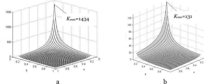
The measurement uncertainty for conductive and elongate particles can be appreciable in the case of smaller particle concentration. We calculated the diapason of factors K_mm and K_nm in the cases of very conductive and nonconductive magnetic particles, correspondingly, using program package Matlab. The values C_a, C_b, and C_c were calculated of Eq. (8) and the values of factors K_mm and K_nm of Eqs. (68) and (72), correspondingly, when c < b < a and the ratios e = b/a and g = c/b were varied in intervals [0.1: 0.95] with the step 0.05. The obtained results are presented in Figure 3. We can see that when ratio between longest and shortest semi-axes of ellipsoidal particles is equal to 100, the factor K_mm can reach 1434, i.e., the measurement error can exceed the admixtures concentration more than thousand times. Such situation is purely theoretical. Very long and thin particles will be crashed in the turbulent flow or they will not rotate. If they will not rotate, the longest dimension will be directed by flow direction, i.e., by axis z. This dimension has not influence to the measurement error that error will not be great.

Figure 3.

Dependence of the shape factors K_mm (a) and K_nm (b) on g and e, when interval of g and e variation is [0.1: 0.95].

We calculated, too, the dependence of the shape factors K_mm by Eq. (69), K_em by Eq. (72), K_nm by Eq. (75), and K_nc by Eq. (82). These results are presented in Tables 1–3 and in Figures 4–6.

a/c	c/b	Ca	Cb	Cc	Kmm	Kem	Knm	Knc
3	0.9	5.65	5.05	1.61	11.15	4.1	1.7	3.1
3	0.8	5.85	4.58	1.64	10.68	4.62	1.68	3.62
3	0.7	6.1	4.16	1.68	10.22	3.98	1.66	2.98
3	0.6	6.4	3.75	1.74	9.92	3.96	1.63	2.96
3	0.5	6.79	3.34	1.81	9.68	3.98	1.61	2.98
3	0.4	7.29	2.96	1.9	9.63	4.11	1.59	3.11
3	0.3	8.32	2.66	1.95	9.66	4.3	1.59	3.3

Table 1.

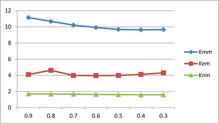
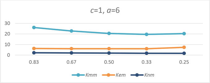
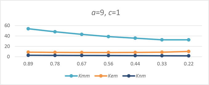
Dependence of the shape factors K_mm, K_em, K_nm, and K_nc on when ratio between longest and shortest ellipsoid semi-axes a/c is equal to 3.

a/c	c/b	Cc	Cb	Ca	Kmm	Kem	Knm	Knc
6	0.83	9.83	7.58	1.3	26.1	6.24	2.2	5.24
6	0.67	10.7	6.63	1.34	22.8	6.06	2.03	5.06
6	0.50	12.1	4.62	1.43	20.5	6.05	1.9	5.05
6	0.33	14.9	3.33	1.59	19.6	6	1.73	5.6
6	0.25	17.6	2.68	1.76	20.3	7.35	1.65	6.35

Table 2.

Dependence of the shape factors K_mm, K_em, K_nm, and K_nc when ratio between longest and shortest ellipsoid semi-axes a/c is equal to 6.

a/c	c/b	Ca	Cb	Cc	Kmm	Kem	Knm	Knc
9	0.89	13.8	11.48	1.19	53.9	8.82	2.83	7.82
9	0.78	14.2	9.81	1.21	48.1	8.4	2.63	7.4
9	0.67	14.9	8.41	1.23	43.1	8.2	2.52	7.2
9	0.56	16.0	6.97	1.26	38.8	8.1	2.36	7.1
9	0.44	17.9	5.6	1.31	35.8	8.3	2.17	7.3
9	0.33	20.5	4.36	1.4	32.6	8.76	1.95	7.8
9	0.22	25.8	3.17	1.54	32.6	10.2	1.78	9.2

Table 3.

Dependence of the shape factors K_mm, K_em, K_nm, and K_nc when ratio between longest and shortest ellipsoid semi-axes c/a is equal to 9.

Figure 4.

Dependence of the shape factors K_mm, K_em, and K_nm on c/b when a/c = 3.

Figure 5.

Dependence of the shape factors K_mm, K_em, and K_nm on c/b when a/c = 6.

Figure 6.

Dependence of the shape factors K_mm, K_em, and K_nm on c/b when a/c = 9.

The particle shape has the great importance to the measurement error when the particles are conductive. We can see that factor K_mm quickly increases with the ellipsoid elongation. If the longest and shortest ellipsoid axes lengths ratio a/c is equal to 9, the K_mm can be between ≈33 when b/c = 5 and ≈54 when b/c = 1.2. Therefore, when the concentration of very magnetic and very conductive particles with such shape will be 1%, the measurement error can reach 50%. Fortunately, this situation is few probable because the measurement error to be so great the concentration of long very magnetic and very conductive particles must be permanent. With the ratio a/c diminution, the factor K_mm quickly decreases. When ratio c/a is not more than 3, the factor K_mm < (11–12). It is not more than two times in comparison with K_mm = 6 for sphere (see [9]).

When electric conductivity of the magnetic particles is comparable with the fluid conductivity, the dependence on the particle shape is less than for very conductive particle but for the particles with ratio c/a > 9 the error can exceed the concentration 10 times.

For nonconductive magnetic particles, the dependence on the particle shape is yet less than for the conductive particle. For sphere the factor K_nm = 1.5, for ellipsoid with a/c = 9 K_nm can reach 2.8.

When the admixture particles are nonmagnetic, the measurement error depends on the particles concentration in second power k². Therefore, the error will be comparable with concentration of the particles when the factor K_nc ≈ 1/k.

9. Discussion

Very different admixtures can contaminate the fluid flow. The measurement’s results will be reliable if we know how the admixtures with the various physical properties influence the measurement results. If we use the electromagnetic flow meters, it is important to know the magnetic and electric features of the admixtures and the shape of the solid admixture particles.

It is convenient to approximate the shape of particles to ellipsoid. By varying lengths of the ellipsoid axes, we can obtain very different spatial profiles: sphere, lamella, cylinder, beam, and other. The ellipsoid has one important advantage for the electric field analysis: when an ellipsoid gets into the homogeneous electric field, there will be the homogeneous field inside the ellipsoid, too. It is a significant property for the analysis of the magnetic field and the virtual current distribution in space with the admixtures. For an effective analysis, the concept of the virtual current proposed by M.Bevir is very important. The virtual current effectively describes the electrical properties of the active zone.

The chosen mathematical tools made it possible to conduct a reliable analysis and find out how various admixtures affect the measurement error.

The performed analysis discovers that the magnetic conductive admixtures are the most dangerous. In this case, the influence of the particle’s shape on the measurement error is maximal. For a very long metallic particle with a length ten times exceeding other dimensions, the error has a huge value of δ_mm = 1434 k. However, the quantity of very long magnetic particles can’t be large. The small particles can’t be very long. The long and narrow particles break quickly in the turbulent flow. In addition, very long particles will not rotate in flow. In this case, the maximal dimension will not influence the measurement error.

We can see that the shape of the particle has a lesser influence on the measurement error of the magnetic particles than the particles that are nonconductive. But for very long particles, it increases too.

The measurement error in fluid with the nonmagnetic admixture particles is proportional to the second power of its concentration. Therefore, it is important if the admixture concentration exceeds 5–10%. The error does not depend on the particle’s shape when the admixtures are nonmagnetic and nonconductive. The shape of the conductive nonmagnetic particles influences the error but not significantly.

This analysis is performed for the turbulent flow. But we can predicate that in the laminar flow, the measurement error by the same admixtures will be not more than in turbulent. The error can arise for long particles. But the long particles will be orientated along the flow direction in laminar flow, i.e., perpendicular to plane xy. In this case, the longest dimension of the particle will be perpendicular to the components J_x, J_y of the virtual current, and to the components B_x, B_y of the magnetic flux density. Therefore, the longest dimension of particles will not influence the measurement error. The total error will be less than in turbulent flow.

10. Conclusions

1. The approximation of admixture particles by ellipsoid allows us to investigate how the shape and physical properties of the admixtures influence measurement accuracy.

2. The equation of the measurement error for the general case was derived. The particular expressions were obtained, too, for magnetic nonconductive and very conductive particles, magnetic particles with conductivity close to the fluid conductivity, nonmagnetic nonconductive particles, and nonmagnetic conductive particles.

3. The maximal error arises when admixtures consist of magnetic and very conductive particles with an elongated shape. When the conductivity of the particles decreases, the particle shape influence on the measurement error decreases too.

4. The measurement error is proportional to the second power of the admixture particle concentration when the particles are nonmagnetic.

5. When particles are nonmagnetic and nonconductive, the measurement error is not depended on the particles shape. The expression for the measurement error coincides with expressions received by other researchers.

References

1.Shercliff JA. Relation between the velocity profile and the sensitivity of electromagnetic flowmeters. Journal of Applied Physics. 1954;25:817-818
2.Bevir MK. The theory of induced voltage electromagnetic flowmeters. Journal of Fluid Mechanics. 1970;43:577-590
3.Baker RC. On the concept of virtual current as a means to enhance verification of electromagnetic flowmeters. Measurement Science and Instrumentation. 2011;10:105403
4.Bevir MK. The predicted effects of red blood cells on electromagnetic flow meter sensitivity. Journal of Physics D: Applied Physics. 1971;4:387-399
5.Bernier RN, Brennen CE. Use of the electromagnetic flowmeter in a two-phase flow. International Journal of Multiphase Flow. 1983;9(3):251-257
6.Murakami M, Maruo K, Yoshiki T. Development of an electromagnetic flowmeter for studying gas-liquid, two-phase flow. International Journal of Chemical Engeneering. 1990;4:699-702
7.Cha J-E, Ahn Y-C, Kim M-H. Flow measurement in an electromagnetic flowmeter in two-phase bubbly and slug flow regimes. Flow Measurement and Instrumentation. 2002;12:329-339
8.Muhamedsalih Y, Lucas GP, Meng YP. Two-phase flow meter for determining water and solids volumetric flow rates in stratified, inclined solids-in-water flows. Flow Measurement and Instrumentation. 2015;45:207-217
9.Virbalis JA. Errors in electromagnetic flow meter with magnetic particles. Flow Measurement and Instrumentation. 2001;12(4):275-282
10.Šimeliūnas R, Virbalis JA. Investigation of field of ellipsoidal shape magnetic particle. Electronics and Electrical Engineering, ISSN 1392-1215. 2002;nr. 7(42):72-77
11.Pakėnas V, Virbalis JA. Influence of non-magnetic amixtures to the signal of electromagnetic flow meter. Electronics and Electrical Engineering, ISSN 1392-1215. 2011;nr. 10(116):7-10
12.Virbalis JA, Račkienė R, Kriuglaitė-Jarašiūnienė, Otas K. The influence of admixtures to the signal of an electromagnetic flow meter. Energies. 2019;12:772. DOI: 10.3390/en12050772
13.Landau LD, Lifshitz EM. Electrodynamics of Continuous Media. Мoskow: Nauka; 1982. p. 620
14.Andre A. Complements de mathematiques. Paris; 1957. p. 708
Written By
R. Račkienė and J.A. Virbalis
Submitted: 13 July 2023Reviewed: 17 July 2023Published: 13 February 2024