A Heartbeat-Interval Time Series Analysis, Modified Detrended Fluctuation Analysis, mDFA, Distinguishes between Stressed- and Happy-Heartbeats: From Invertebrate Animals to Humans

Abstract

This study provides evidence that a time series analysis (modified detrended fluctuation analysis, mDFA) is practically distinguish happy- and stressed hearts. This endures that the scaling exponent (scaling index, SI, or alpha, α) can characterize the state of heartbeats. We learned from various challenges of case studies; for example, the Wolff–Parkinson–White syndrome yields a high SI (way surpass 2.0) while feeling sick condition, but the same heart exhibits a healthy SI (∼1.0) when the heartbeats return to normal. Meantime, a healthy SI (∼1.0) goes down to a low SI (0.7) when truly enjoying meal. It seems that SI can represent invisible internal world. The complex interaction between the cardiac rhythm and the autonomic brain command becomes perceptible by the SI. Our observations confirm the state of the heart is measurable quantitatively. A time series analysis of mDFA can help holistic understanding of the brain-heart axis.

1. Introduction

The cardiovascular system includes the heart, intrinsic nerve ganglia, and afferent/efferent extrinsic nerves. It maintains brain-heart health [1, 2, 3]. When it goes wrong, we get sick. It is a life-threatening cardiovascular disease (CVD) in the worst-case scenario.

CVD is caused by changes in the qualitative dynamics of physiological control systems [4]. Earlier detection of a sign of changes at the beginning of a disease (i.e., silent onset of a disease) is ideal if we oppose it. The changes often lead to alterations of rhythm, from normal one to pathological ones. Actually, it is said that beat-to-beat variations of heart rate reflect the sign of changes [5].

In the 1990s, Peng et al. [6] proposed the idea that heartbeat time series analysis helps reduce CVD. In clinical medicine today, however, can we decode the fluctuations in physiological rhythms to better diagnose human disease? The answer to the question is, No. Leon Glass [7] mentioned: The mathematical analyses of temporal properties of physiological rhythms have not yet led to medical advances. Others also said that the mathematical rhythm analysis is still far away from clinical medicine, and clinical utility is not established [8].

In short, a mathematical understanding of the complex fluctuations of cardiac rhythms has been unsuccessful in predicting a heart attack. In fact, the US Preventive Task Force (USPSTF) recommended against screening with the electrocardiogram (EKG) to prevent CVD events in asymptomatic adults at low risk of CVD events (see the latest USPSTF in 2022 as well as in 2018 [9, 10]).

However, since Einthoven’s invention of EKG, EKG has become a recognized electrophysiological technique (see PQRST EKG wave, Figure 1A). Today, EKG is a canonical method of testing/diagnosing/understanding the diseased heart.

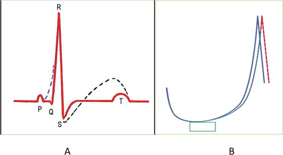
Figure 1.

(A) Diagrammatic representation of EKG waves (PQRST) showing normal (red line) and abnormal (dotted lines in blue and black) states. (B) Diagrammatic representation of action potentials (AP, intracellular membrane potential) of excitable cells such as myocardial cells and nerve cells. Note the unstable peak time of AP. Depolarizing stimulation slightly above the threshold (green square period) induces two superimposed action potentials (blue and red).

By observing abnormal configurations of EKGs (Figure 1), medical doctors can get diagnostic ideas: for example, Wolff–Parkinson–White syndrome (WPW syndrome, blue dotted line) and ST segment issues (elevation or depression, black dotted line). The doctors can measure the abnormality of the Q-T interval, if any. So, EKG is a useful diagnostic tool. Despite this, the USPSTF recommended against “screening” with EKG, as mentioned above.

Now, questions arise. What is wrong with EKG (i.e., heartbeat data) for screening? Does heart rate variability (HRV) analysis, which is based on EKGs, has any problem with screening? Our answer is: problems might be data-collection- or data analysis methods, which would blur the boundary/distinction between the healthy and pathological data.

As neurobiologists, we consider that sophisticated HRV researchers (e.g., physicists or mathematicians) use EKGs not collected by themselves. So, they might not be sure precisely the circumstances when the EKGs were taken. We decided that we must collect EKGs by ourselves, and we did so in the present project (which started around 2000).

We have already shown the distinction between the healthy and pathological data using model animals, crustaceans [11, 12]. We reported that heartbeat time series constructed from EKG contribute to understanding the cardiovascular system [11, 12].

Although the USPSTF says that EKG has no benefits in the assessment of future CVD risk, we feel sure that EKG carries invisible information to understand the cardiovascular regulatory system. For the practical use of EKG in medicine, we report that reliable data and reliable data analysis will not blur the distinction between healthy and pathological data. We thus propose an idea regarding the time series analysis of heartbeat data. This has been conceived from neurobiological experiments.

2. Method

2.1 Accuracy and fidelity in sampling raw EKG

2.1.1 Sampling frequency: sampling rate

As shown in Figure 1B, neurobiologists have experiences: the period length from the onset of stimulation to the peak of the action potential is not stable but changeable. The peak time of the action potential fluctuates each time after the same stimulation. In particular, the fluctuation can be seen when being stimulated just above threshold depolarization. In the brain-heart axis, this fluctuation might cause fluctuation in heartbeat intervals. Therefore, heartbeat-interval time series involves complex fluctuations due to constantly changing subsystems in the complex cardioregulatory mechanisms, including neurotransmitters, ion channels, excitation–contraction coupling of myocardial cells, etc.

In a neuronal cell, the minimum fluctuation ranges 1–10 ms (e.g., Figure 2A shown in Ref. [13]). In a myocardial cell, the fluctuation ranges up to 50 ms (e.g., Figure 4 of Widemann’s paper [14]).

From the above consideration, we determined our sampling rate 1 KHz (every 1 ms) to capture high-fidelity fluctuations.

2.1.2 EKG amplifier and input time constant (τ)

Internationally, the time constant for EKG amplifier is determined as a few seconds (3.2 sec in Japan Industrial Standard). Thanks to this “slow” time constant, we can easily recognize the appearance of abnormal traces (relatively slowly changing voltage traces) in EKG, such as Figure 1A blue and black lines. However, if a patient moves during EKG recording, strong movement generates a large noise (see white arrows in Figure 2) that induces scaling out from the screen of PC (see Figure 2A). In such occasions, a part of EKG’s voltage traces are not recorded. In short, a few heartbeats are not registered (see Figure 2A, heartbeats numbered 3, 4, 5, and 6, shown in black). Thus, slow time constant machines lead to imperfect data acquisition if individuals move. Then, we fail to construct an accurate heartbeat time series.

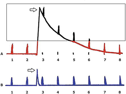
Figure 2.

Diagrammatic explanation for the time constant (τ) of input of an EKG amplifier. A, τ = 5 s, B, τ = 0.1 s. arrows indicate noise abruptly induced by the body movement. Square area data is not registered due to scaling out.

For that reason, we determined our EKG amplifier has a small time constant (0.1 s), as shown in Figure 2B. Here, a large movement noise does not induce a large scaling out phenomenon (white arrow in Figure 2B). Figure 3 shows our EKG amplifier’s electric circuit, no other fancy circuit such as a hum-filter was added. The capacitance of the input capacitor is 0.1 μF and the resistance of the input resistor is 1 MΩ. Therefore, input time constant τ is 0.1 s (C × F = 0.1 × 1) (Figure 3).

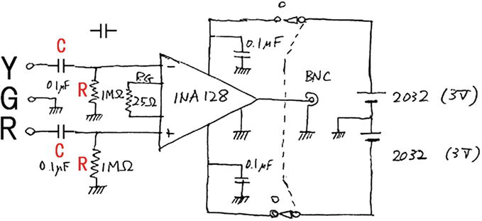
Figure 3.

EKG amplifier circuit, diagrammatically demonstrating the input time constant (τ). Here, τ = C × R = 0.1 s. (C, 0.1 μF. R, 1 MΩ). Courtesy of prof. Dr. Yukio Shimoda, Tokyo Women’s medical university. See Figure 4 for the contact pins Y, G, and R.

Figure 4 shows how to record EKG. Three disposable EKG electrodes (R, G, and Y) (Vitrode V, Nihonkoden, Tokyo, Japan) are attached to the body, and lead cables (carbon fiber) are connected to the EKG amplifier. The EKG amplifier is put in a pocket of individuals, and EKG signal is sent through a long cable (5 m) to the logger (PowerLab, AD Instruments, Australia). Therefore, individuals can freely walk around across 10 m circle area (Figure 4). Output from the digital logger is stored in PC.

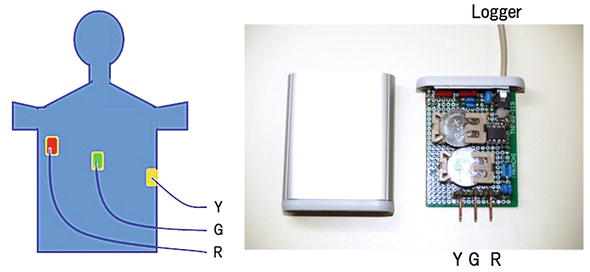
Figure 4.

EKG setup: Commercially available electrodes and self-made amplifier.

From these methods, we can capture accurate and high-fidelity EKG data. To date, we met over 400 different individuals to record EKGs, all of them outside the hospital. As for invertebrate EKG recordings, we already have over 1000 data. All EKG collections were conducted according to the ethical code of the university (see also Figure 5).

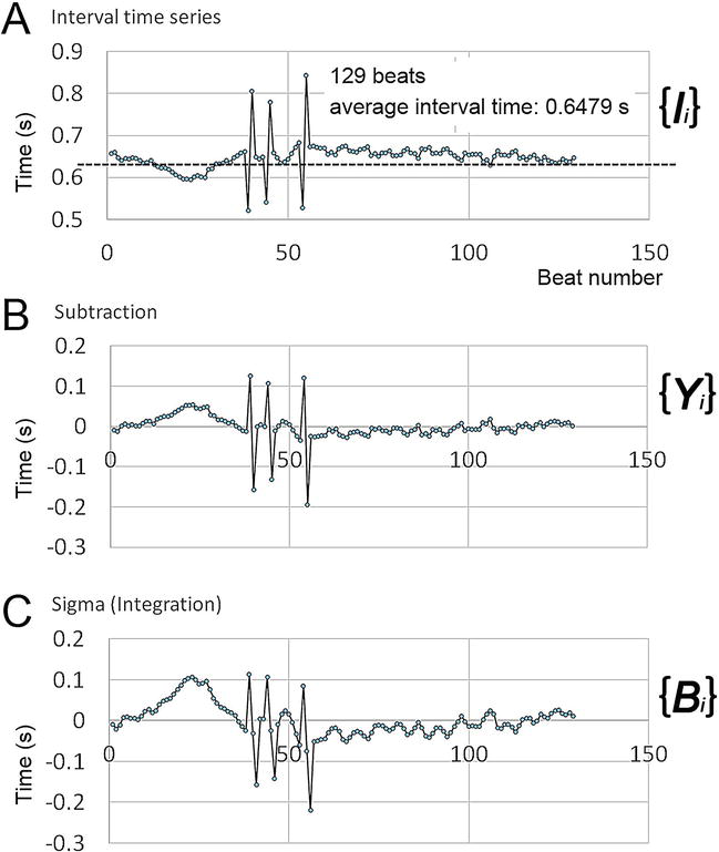
Figure 5.

Preprocessing for mDFA (see text). Volunteer: German in her 50s. Three arrhythmic heartbeats, premature ventricular contractions (PVCs) are included (volunteer subjects put their sign on a written certificate. The statement of mutual agreement describes that EKGs are used only for research and hold out no traceability of personal information. The human heartbeats were recorded outside of a hospital, in for example university laboratories and convention halls - the innovation Japan exhibition. All subjects were treated as per the ethical control regulations of the universities, Tokyo Metropolitan University; Tokyo Women’s medical university).

2.2 Construction of the heartbeat-interval time series

Figure 6A shows EKG data recorded by PowerLab. We format EKG as Text, that is, a voltage vs. time data set by the PowerLab program. Then, we transfer it to our own program, which captures R-peaks (Figure 6B), and construct heartbeat-interval time series (Figure 6C). If the program captures an inaccurate R-peak, such as noses, we make changes by eyes (Figure 7). We do this on every EKG. Thus, the present study accurately captured all of the biological R-peaks. Thus, the authenticity of the time series is ensured.

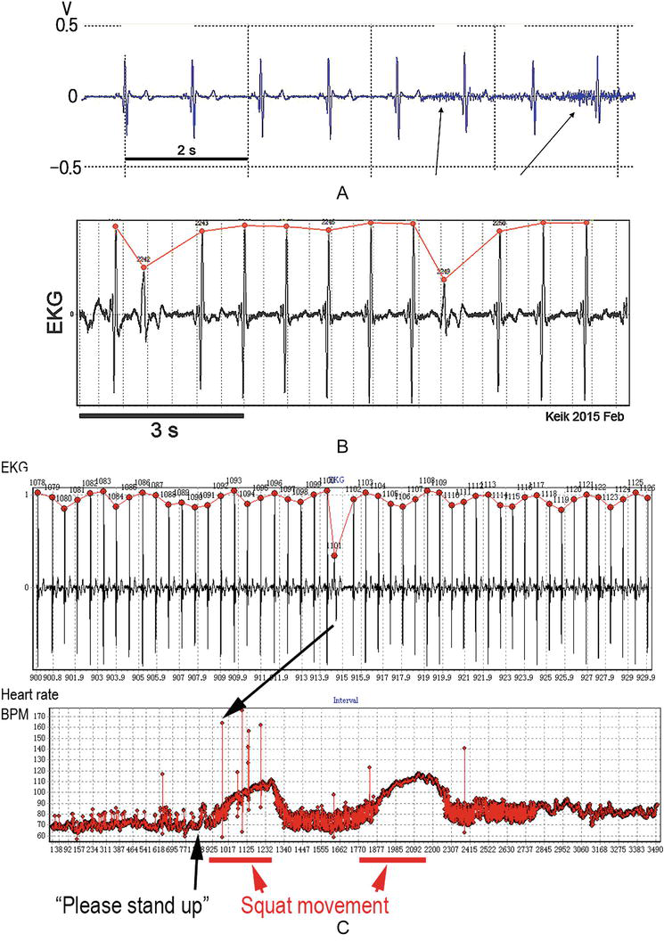
Figure 6.

(A) A raw EKG recorded by the amplifier with input τ = 0.1 s. note, despite the subject raised hands up and down, the EKG baseline is stable with very small noises (arrows). (B) R-peak detections with our program (points in red). (C) Calculation of peak-to-peak interval time, constructing the heart rate time series (beats per min, BPM) or interval time series (not shown). Note that a subject is asked to stand up from a chair and do two sets of 50-time squatting.

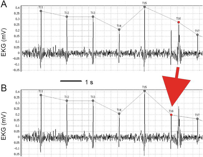
Figure 7.

Correction of a false peak (an arrow). (A) False. (B) Correct. We do all corrections manually by eye observation on the PC screen.

2.3 Time series analysis

2.3.1 Crustacean model animals

On the spiny lobster heartbeats, we have reported that the isolated heart (natural brain control is lost) and the intact heart (neuronal and neurohumoral control are intact) are distinguishable from each other [11, 12]. In the report [12], we used a method, detrended fluctuation analysis (DFA) proposed by Peng et al. [6, 15], and found that DFA is a good method to distinguish between a healthy heartbeat and an abnormal heartbeat of a model animal. But, unfortunately, as mentioned above, heartbeat rhythm analysis is still not remarkably contributing to clinical medicine [7, 8, 9, 10].

After studying the details of the computation procedures of DFA (see [6, 15] for a full explanation of DFA), we made a new method with a different concept based on neurobiological experiments.

DFA deals with “critical” phenomena existing in nature. We understand why Peng et al. [6] focused on “criticality” of a diseased heart [6, 15] because “sudden” heart attack is a big health issue, in cardiac medicine. However, for normal people, it is rare that the heartbeats suddenly encounter a critical moment. We created a different method, modified detrended fluctuation analysis (mDFA) [16, 17] with neurobiological thinking.

2.3.2 mDFA: data preparation

Each EKG recording is a long-lasting continuous recording, spanning over 30 min to 10 hr. or more in our project. The peak checking on the PC screen is formidable work, but the peak accuracy is necessary condition (Figure 7). Peak-capture failure surely messes up the “statistical” conclusions. Many results have been reported by “highly sophisticated physical” methods. We want to avoid inaccurate data preparation.

We only use the heartbeat-interval time series constructed in our lab. mDFA would otherwise ultimately yield a monstrous result. Perfect logging and accurate peak-to-peak sampling are ideal.

2.3.3 mDFA and DFA: algorithm

There are important conceptual differences in the algorithm between DFA and mDFA that were already mentioned elsewhere in 2015 and 2019 [16, 17]. Here, we shall explain it briefly.

Figure 5A shows the time series {Ii}. This is the set of times for peak-to-peak intervals. Figure 5A involves 129 interval data, from I₁ to I₁₂₉.

The dotted line is the average of interval time from 129 intervals. Here, the average value < I > is 0.6479 s.

Figure 5B shows the set {Yi}. This is the set of times of “real” fluctuations calculated as: {Yi} = < I > − Ii. Either (Yi = Ii - < I >) or (Yi = <I > − Ii) can be usable. But if squared, (< I > − Ii)² = (Ii - < I >)², both became equal.

Next, Figure 5C shows the integrated time series, that is, {Bi} = ${\sum }_{\mathrm{k}=1}^{129}Y\mathrm{k}$. Here, the integration process, adding each value of {Yi} successively, is plotted.

Interestingly, it is remarkable that a time segment of “persistent acceleration” or “persistent inhibition (deceleration)” is intensified by the integration (see beat numbers ranging over 1–40, Figure 5C).

In contrast, sporadically appearing events, that is, PVCs, are not intensified (see three PVCs, Figure 5C). Therefore, persistently occurring events (autonomic acceleration or deceleration) and sporadically occurring events (arrhythmic heartbeats) may have different effects on mDFA outcomes. But, without time series analysis, little is transparently noticeable when watching EKG alone. The time series data is so great and of interest.

The “sigma or integration” method is the most important step of mDFA. The trajectory of the set {Bi} is more dynamic than {Yi} (Figure 5B and C). Again, constructing the set {Bi} is the key step for mDFA (and DFA as well). It is a random walk-like analysis concept.

2.3.4 mDFA: fitting

In mDFA, the integrated time series {Bi} includes 2000 sets of times. Practically, it takes at least 30 min for EKG recording.

In DFA, not mDFA, the integrated time series {Bi} is divided into boxes of equal length n, and a least squares line is fit to the data.

However, in mDFA, {Bi} is NOT divided into boxes of equal length n before the fitting to the data. In mDFA, at first, the biquadratic fitting line is made, then divided into box of equal length n. There are n samples in a box.

We have tested linear, quadratic, cubic, fourth-degree polynomial, fifth, sixth, etc. The results of linear, quadratic, and cubic fittings were scattered. At a greater than fourth degree polynomial fitting, the resulting scaling exponent is converged to a number. In mDFA, therefore, a biquadratic curve fitting is used (Figure 8).

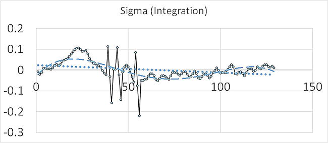
Figure 8.

An example least squares line fit to the data. Fitted curves: Dotted line (…), linear fitting, and dashed line (− − −), biquadratic fitting. Here, the number of heartbeats shown is only 129 beats. In mDFA, biquadratic fitting line is made from 2000 data, instead of within a box. Peng’s DFA, however, makes the fitting line within individual boxes (see Peng et al. [6] for the details of “box”).

2.3.5 mDFA: detrending

Computation of a least squares line fit (LSLF) to the data {Bi} reveals the trend line (Figure 9A). In mDFA, the trend line is a biquadratic line, but here we will use linear fitting for the sake of convenience. We detrend the interval data {Bi} by subtracting the trend (Figure 9B).

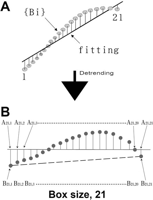
Figure 9.

Diagrammatic explanation of detrending. (A) the set {Bi} is a set of times. A fitting straight line is linear fitting. Although mDFA uses biquadratic fitting instead of linear fitting, we here use linear fitting for the sake of convenience. An arrow from A to B, the subtractions, “{Bi} – Fitting” that is a detrending process. (B) Diagrammatic representation of the difference between mDFA and DFA (see text).

In the DFA algorithm, LSLF is made in each box, but in the mDFA algorithm, LSLF is done upon entire interval data {Bi}. Why do we do so? Because we consider that the heartbeat change is a continuous phenomenon. Past incidences always affect future incidences to a lesser or greater degree. So, the first heartbeat in a time series has an influence on following heartbeats to a lesser or greater degree. Therefore, when drawing a fitting line (LSLF), mDFA computes the entire trend at once, not inside a box, as DFA does (representing the trend in that box). This notion of mDFA is a totally different concept from Peng’s DFA concept.

2.3.6 mDFA: root mean square and box size

Imagine, in the eq. Y = a × X, a determines the slope in the X vs. Y graph. A linear relationship exists between Y and X. Also, logY = a × logX, where a also gives the slope. This equation is compatible to the eq. Y = X^a. It is a double-log plotting graph. A linear relationship on a double-log graph indicates the presence of scaling, that is, F(n) = n^α. The scaling index α can be determined from a log-log graph. (Abbreviation for the scaling index; we use SI or α).

In Figure 9B, the box size n is 21. The differences between {Bi} and fit line are, A_21,1 – B_21,1, A_21,2 – B_21,2, A_21,3 – B_21,3, − − −, that is, the length of vertical lines in Figure 9B (see vertical straight line segments in Figure 9B).

If A > B, A – B gives a positive value, and if A < B, A – B returns a negative value. Therefore, when we consider the average value of (A – B), we use the root mean square, which is F² = < (A −B)² >, as a matter of practical convenience. This calculation is what Peng’s DFA program does. This computation is repeated over all of the box sizes to provide a relationship between F and n.

In contrast to the DFA algorithm, mDFA algorithm does not use A – B. Instead, mDFA uses subtractions B_21,1 – B_21,21 in one box, where the box size is 21 (see the dashed line in Figure 9B). So, B_21,1 is the first data of the box (Entrance), and B_21,21 is the last data of the box (Exit). Therefore, mDFA computes the subtraction (Entrance – Exit), or the difference between the value of Entrance and the value of the Exit. This computation is repeated over all of the box sizes to provide a relationship between F and n.

Why do we do so? The answer is: we want to illuminate the phenomena more slowly, varying with time. Vertical subtraction A – B focuses on the critical moment of relevant issues, that is, cross-section of time. In contrast, the subduction (Entrance – Exit) is focusing on phenomena varying with time, that is, focusing on segment of time. This is one of the biggest algorithm differences between mDFA and DFA.

2.3.7 mDFA: the scacling law does not govern the entire domain (window size, domain size, margin, or boundary)

Peng and Goldberger et al. [6, 15] mention that DFA works on time series data that has fractal-like characteristics or self-similar structure. They also mention that they prefer to use a longer data. The longer, the better. They used 24 hr-length data with a Holter EKG monitor [6, 15].

Our body system is never run stable for 24 hr. It rather changes momentarily. In our everyday life, we can concentrate on a thing (one object, song, program, etc.) for a limited period. Our mind changes dynamically from one thing to the next. The stability of the brain-heart axis might last only for a short period. Imagine humans can keep continuing a steady state: a boxing-fighting game consists of 3 min for one round; we wait 3 min before a pot noodle becomes ready to eat; a popular music hit-the-charts, for example, “Take Me Home, Country Road” lasts for a perfect (not too long and not too short) length “three” min; and so forth.

In physics, ideally, the scaling law holds across a whole length of data set in the steady state condition. But, in biology, we consider, scaling will appear in a limited period length. In the current experiments, we wanted to find the period length, that is, window size or domain size, or margin or boundary, which is autonomously regulated. Within this length, we see the steady state of the body system.

From our experiences, for capturing “biologically true scaling index provided by the steady state of the body,” we found a 2000 consecutive heartbeat data is adequate in length. In mDFA, the box size length (l) is fixed as: 10, 11, 12, − 18, 19, 20, 21, 22, − 99, 100, 110, − 190, 200, 210, 220, − 290, 300, 310, 320, − 480, 490, 500, 600, 700, 800, 900, and 1000 (BPM).

After that, the scaling index is calculated using a restricted window size of log–log graph, that is, box size length stretching out from 30 to 270, depicted as [30; 270], or the domain of definition 30 < l < 270, in our projects (see [6, 15]).

In the regulation of heart rate, scaling characteristics of heartbeats will appear in the domain around “three” min. This size is in line with two decade in logarithmic scale, that is, between 10 BPM and 1000 BPM (BPM, beats per min). The scaling index is computed from a double logarithmic graph [6]. We, therefore, studied heartbeats during these two decade.

In the textbook definition, in healthy human individuals, heart rate at rest ranges from 50 to 100 BPM. So, the number of three-minute heartbeats corresponds to 150–300. The window size [30; 270] does not miss the point in terms of neurobiological considerations (see the graph Figure 10B for the scaling computation, that is, section length of linear fitting straight line).

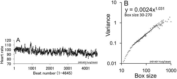
Figure 10.

mDFA’s log–log graphic demonstration (see [16, 17, 18] for detail). (A) Time series of 4645 beats, from a healthy happy individual in her 50s (no skipping or arrhythmic beats, laughing, and talkative while recording this EKG). (B) Log–log plotting in order to calculate the slop. A fitting line is made from box size 30 to box size 270, that is, frame size [30; 270], not beyond this size. We reached a conclusion: This window size best captures the scaling exponent that fits the biological explanation regarding the state of the heart. Here, SI = 1.031. So, mDFA works at the restrictive span of dimension [30; 270].

In conclusion, the best window size, that is, the domain 30 < l < 270, ensures that mDFA gives a reliable and satisfactory useful scaling index, as shown in the results section below. Our mind might be quantified by the scaling index [18, 19]. We can peer into the mind through a window. The size/length will be a period of approximately 3 min. We applied mDFA in various disciplines, including the heart, material vibration, and earthquake [6, 15]. The window size [30; 270], that is, the domain 30 < l < 270, is universal. As a practical tool for time series analysis, mDFA’s window size is important to guarantee the reliability of mDFA.

2.3.8 mDFA: coda

What Peng’s DFA characterizes is conceptually different from what mDFA characterizes. The former characterizes criticality phenomenon, the latter characterizes phenomena more time-change dependent than DFA does. Every happening in the world has causation. The causation is often hidden or merely cannot be seen or hardly detected by human sensory-brain ability. Some causalities are invisible like the silent onset of disease. Some causalities are explosive and appear suddenly. Peng’s DFA can see critical solutions. mDFA may see the relationship between the past and the present life. The heart could not be a good field for criticality physics, but the brain is the most appropriate field because we often experience “Aha!” or eureka moment [20].

3. Results

3.1 Case study: unhappy heart, WPW syndrome

A recording set shown in Figure 3 was used. Tachycardia (fast heartbeat) and arrhythmia are two of the many common heart problems today.

If a fast heartbeat occurs acutely and suddenly, the heart becomes an inefficient pump. Enough blood is not pumped to the brain, making the person feel sick. It is also life-threatening.

We recorded a fast heartbeat EKG from a girl who suffered from WPW syndrome (Wolff-Parkinson-White syndrome). She is approximately 10 years old. The family, parents, and children have moved to United States from Cuba to receive medical care for heart problems. We met them a few times in a town Great Falls near the Potomac River.

Her mother explained that the girl feels ill when a tachyarrhythmia seizure occurs. We saw her running into a washroom when she had an unpleasant sensation.

Figure 11 shows the interval time series of the young girl. In Figure 11A and B, the seizure is recorded. She did not tell me about feeling funny at that time, although her face looked sick to me. Later, when we checked the data, we understood that the seizure did not last long. It was only approximately 20-heartbeats (Figure 11C).

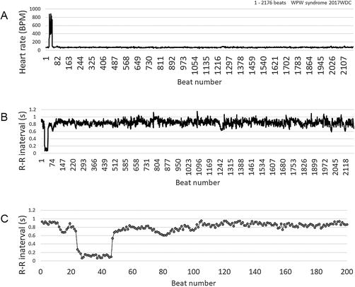
Figure 11.

Time series constructed from WPW syndrome of a young girl. About 10 years of age. Abrupt seizure is recorded in the initial part of the time series. (A) Heart rate time series, 1–2176 beats. (B) Converted to the peak-to-peak interval. (C) Initial part of the interval time series, 1–200 beats.

Figure 12 shows mDFA results. The seizure increases SI (scaling index, scaling exponent) value significantly. Her mother told me that her daughter is expected to receive catheter ablation next week. It will be the third time. In the two previous treatments, nothing was effective. She asked: “Do you think should I take her to the hospital again?”

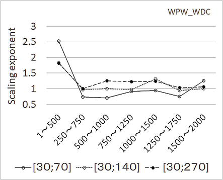
Figure 12.

mDFA results on the WPW syndrome data shown in Figure 11. The data length for mDFA computation is 500 beats. Computation was displaced in sequence every 250 beats. Note: The seizure (the period 1–500) evidently and significantly increases SI (scaling exponent) values. Three different box sizes [30; 70], [30; 140], and [30; 270] are shown here, although generally, we use [30; 270].

I replied: “My wife’s friend has a husband who has a similar condition as the girl. He, the husband, fell over in the road before, and an ambulance saved him. He already received twenty (20) catheter ablations. Unfortunately, it never worked. He went to see a new doctor in a different hospital where a celebrated cardiologist was working. And then, the latest catheter ablation totally removed the arrhythmia. Please do not abandon hope.”

One month after my mDFA recording, the girl’s tachycardia disappeared after the third catheter ablation, of which I was notified by an e-mail.

For more results with this method, please consult [18], such as “Bundle Branch Block, Problems in the Electrical Conduction System of the Heart”.

3.2 Case study: healthy happy heart—working-eating-exercising

A recording set shown in Figure 3 was used. Figure 13 is an example of a cyclically computed mDFA upon a volunteer subject in her 60s. Figure 13 shows a working-eating-exercising mDFA. She kindly offered herself to the EKG recording twice a week, and for years when she worked in the laboratory. Her time series exhibits many PVCs. These PVCs are benign. While she is working on PC (1–3000), she has a low exponent, which means she is concentrating on the job. It is seen that she is working earnestly. When I showed her Figure 13, she told me that mDFA is scary because someone indeed can look at my internal world, my mind. During meal time (lunch, 6001–9000), the exponent noticeably decreased. Exercise (9000–15,000) elevated the scaling exponents significantly. This test supports the hypothesis that mDFA can quantify the mind.

Figure 13.

An employee’s EKG recording and mDFA. Volunteer subject, in her 60s. Inset time series shows 15,000-beat data while working on PC, having lunch meals, and squatting (SQ) three times, each 50-squattings. Many PVCs are occurring. These PVCs are benign – 60 percent people over age 40 have this PVCs (premature ventricular contractions). For every 3000 beats, SI values were computed. Working time, a low exponent. During meal time (lunch), the exponent noticeably decreased. Exercise elevated the scaling exponents significantly.

In conclusion, concentration on the job lowers the scaling exponent from normal healthy exponent 1.0 down to 0.9 or lower. This observation does not contradict previous results which were found by employees at the Indonesian University [18]: People who are the president of the University, Vice president of the University, and the Dean of faculty all of them had a low exponent (SI = 0.72–0.84). They are relatively seriously talking to me with dignity during the EKG recording. In turn, ordinary employees (teaching only professors who were happily talking while EKG recording) had a healthy exponent (SI = 1.0) [18].

3.3 Case study: passenger’s mDFA. EKG monitoring during in flight

A recording set shown in Figure 14 was used. In the flight frying from Tokyo, Japan to Washington DC (WDC), Virginia, USA, mDFA found: (1) Wine service significantly decrease the scaling exponent (Figure 15, data number 4). (2) Sleepy conditions lower the scaling exponent (Figure 15, data numbers 7, 8, and 9). (3) A boring movie (i.e., sleeping) also decreased the scaling exponent, but an interesting movie does not (Figure 15, data numbers 12, 13, and 14). Fundamentally the same results were obtained by the returning flight and the next Tokyo-WDC flights too (data not shown). In other “mobile EKG—mDFA” confirmed that the happily eating condition (such as Figure 13, the value at 6001–9000) and sleepy condition lowers the scaling exponent (data not shown).

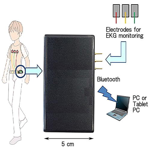
Figure 14.

An EKG monitoring set using the Bluetooth radio wave. Individuals can carry an EKG monitor in their pocket. The monitor sends authentic EKG waves to PC. EKG electrodes and EKG amplifier are the same, as shown in Figure 4.

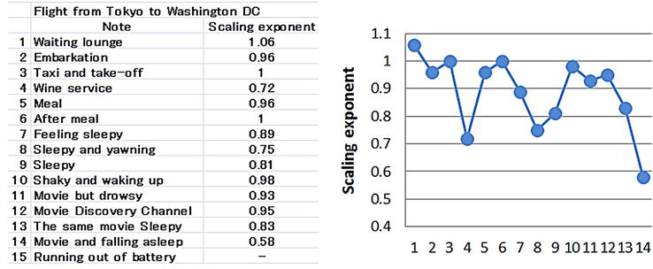
Figure 15.

EKG-mDFA cyclical challenge during a flight. EKG monitoring method is shown in Figure 14. mDFA computation was done after the flight. From 1 to 14, each data has 2000 heartbeats. Note, record numbers 5 and 6: Having a meal but enjoying conversation with people next seat; SI does not decrease. Record number 15: Experiments failed due to running out of amplifier battery.

We have also tested “mobile EKG—mDFA” in the passenger aircraft from Orland, Florida, to WDC. It was of interest that, in the landing shaky aircraft in bad weather, feeling-scared states lowered the scaling exponent, but the scaling exponent recovered autonomously to a normal exponent (i.e., SI = approximately 1.0) after touching down on the runway (see Figure 63 of [18]).

4. Discussion

4.1 Accuracy and fidelity of the time series construction

In the present communication, we present how to record high-fidelity EKG and how to construct accurate heartbeat-interval time series (Figures 4–7). For the steady progress of clinical medicine, especially for diagnosing and managing patients, people like sophisticated physicists (e.g., [5, 21]) require to analyze the accurate time series, instead of easily available data (e.g., [22]). In the [22], authors mentioned that “a gap resulting from artifacts, noise, and exclusions of ectopic beats was considered equal to the R-R interval subsequent to the gap.” And they continued by mentioning that “the length of interpolated gaps relative to the total length of the recording was 0.024%.” We are, however, apprehensive about the “interpolation” of the gap. Such artificial data processing might break up authentic phenomena. It is not true data. In preparing data, false or true is a matter. We cannot ignore artificial alteration, even though it is very little, 0.024%. Our time series, it is so real.

In the article [15], similar modifications of missing heartbeats were done (the gap was supplemented [15], or the gap was removed [23]). To enhance trust in clinical medicine, especially for diagnosing and managing asymptomatic patients (i.e., early detection is the best way), high-tech physicists must fully fill a requirement: constructing high-fidelity time series data.

4.2 Our past experiences influence our current perceptions

Both DFA and mDFA use a subtraction, that is, (B – A) or (Q – P), respectively, as I already explained in Figure 9B. The former corresponds to DFA algorithm, and the latter corresponds to mDFA argorithm.

Both methods calculate a “mean value”. The mean value is not a simple average but the mean-square, that is, (B – A)² or (Q – P)², respectively. Due to the usage of mean-square, this scaling analysis uses a graph of the double-log plotting, as mentioned. Both methods repeat computations cyclically over and over all the box sizes. Finally, the relation between F(n) and n is plotted on the double-log graph, as mentioned. This provides a relationship between F(n) and n. The slope of the graph determines the scaling exponent in both DFA and mDFA.

However, the concepts behind computations are different each others between DFA and mDFA. DFA calculates (B – A), but mDFA calculates (Q – P) instead. The former’s concept suggests criticality or tipping point phenomena. In contrast, the latter seeks the random walk-like concept, that is, “how many steps proceeded in a box.” This involves, neurobiologically, an idea: “Our past experiences influence our current perceptions.” This is the main point of the computational concept of mDFA (Figure 16) (see [18]).

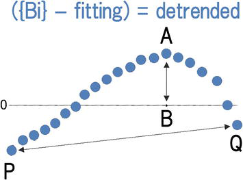
Figure 16.

Diagrammatic representation regarding the difference between DFA and mDFA. Modified from Figure 9B. DFA uses subtraction (B – A). mDFA uses the subtraction (Q – P).

4.3 Fractal the self-similar structure but restrictive span of dimensions

Heartbeat series shows self-similar structures and self-similar fluctuations [24]. Likewise, the tree-like spatial fractal has self-similar branchings: The small-scale structure resembles the large-scale form [24] (see A, B, and C in Figure 17). In the heart regulation, a fractal temporal process may generate fluctuations on different time scales that are statistically self-similar [24]. But, in biology, self-similarity appears only in restrictive span of dimensions, as shown in Figure 17.

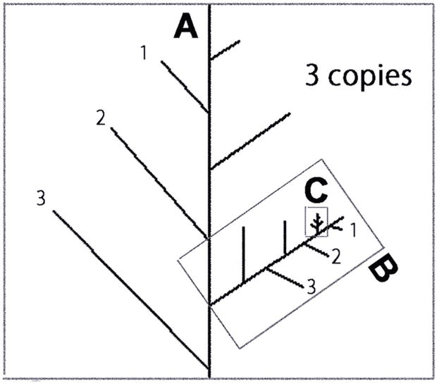
Figure 17.

Diagrammatic representation of tree-like self-similar branchings. The small-scale structure resembles the large-scale form (A, B, and C). In a real country field, there are NO trees larger scale than A, and NO smaller scale than C. In biology, scaling appears in a limited size; meantime, the size can grow up to infinity in ideal physics. Dimension should be adjusted to real size (window size, or tree size) to measure the scaling index in the self-similar real data.

mDFA looks at restrictive span of dimension or restrictive frame size or box size, that is, confined window size [30; 270] or the domain 30 < l < 270 (see Figure 10B). A linear fitting line (see Figure 10B) does not extend beyond the framework [30; 270]. mDFA do not consider boxes smaller than 30 and larger than 270 when determining the scaling exponent in its computation. We actually tried various set of “frameworks” before reaching this conclusion. We finally found that, in this restrictive window size, mDFA is best fit to distinguishing various heart conditions, from healthy happy hearts to other hearts such as stressed- and diseased hearts. Thus, we temporarily conclude that mDFA is successful and acceptable as an efficient tool in the neurobiology of the cardio-regulatory system. Using mDFA, we can tell the distinction between happy hearts and stressed hearts, or between the hearts of natural death and unpredictable death [16, 17, 18].

4.4 mDFA identifies risky and unhappy hearts

From our experimental evidence, mDFA seems to work over a wide range of the scaling exponent, from the value near zero (which can be seen on a smoothly running electric motor) to the value surpass 2.0 (which can be seen on the heartbeats at unpleasant psychological state caused by the WPW syndrome, where the brain cannot receive enough oxygen supply from the heart) (Figures 11 and 12) [16, 17, 18]. Furthermore, the scaling exponent of a girl suffering from WPW syndrome quickly returns to a normal value, around 1.0, after abnormal heartbeat disappeared, that is, coming back to a normal heart condition (Figures 11 and 12). So, it appears that mDFA ensures high fidelity response to the behavior of internal complex system, which is changing its performance moment by moment.

Higher scaling exponents greater than 1.2 are of interest: Surprisingly, higher values indicate that the system is “approaching danger.” This was proven by the nonheart experiments. We applied mDFA on the material vibration, recorded from aluminum rod experiments, where a rod irreversibly bent (snapping off) by the externally applied force. Here, mDFA proved that when the scaling exponent exceeded ca. 1.2, a rod was completely broken (see [17] for details).

Furthermore, we have already reported (Figure 5–22 in [16], p. 62) that terminal patients show high scaling exponents (around 1.5) before dying: The patients suffered from, (No. 1) hepatic cirrhosis, (No. 2) type 2 diabetes plus brain infarction, and (No. 3) colorectal cancer [16]. Meantime, No. 4 terminal patient maintained a lower exponent (∼ 0.5) all the time before dying. She suffered from senile weakness. So, three patients (No. 1–3) died “unpredictably.” But, in the case of No. 4, the doctor’s gut instincts can “sense” that “something” will happen sooner or later. (We are grateful to Dr. K. T. at Kojimachi, Yotsuya, Tokyo, for providing us EKG data of terminal patients. He equipped his special EKG monitoring machine on patients, and patient’s EKGs were seamlessly sent to the PC in his clinic office through the mobile-phone internet network. He does not take the patient to the office; instead, his office has an uninterrupted EKG online connection to the patients at home [16]. Time series data were constructed by us, and mDFA also by us.)

In summary, evidence indicates that higher scaling exponent way exceeding 1.2 could be showing unhappy (risky) state, either in human heart or material structures.

4.5 mDFA during working, eating, and doing exercise

The heartbeats during a job exhibit a low scaling exponent (0.8–0.9 in Figure 13). This does not contradict with the previous report, which showed that serious employees of the university, the president, vice president, and faculty dean, all exhibited a low scaling exponent [16] as mentioned above.

The heartbeats during happy lunch exhibit a low scaling exponent (0.7, Figure 13; 0.7, Figure 15 during wine service).

But having meal and enjoying conversation with people next seat does not decrease SI (Figure 14, record numbers 5 and 6). Here, the brain does not concentrate on meal, and the scaling exponent was not noticeably altered. The previous report also supports this interpretation of “having meal mDFA” (see Figure 14 of previous publication [19]). If individuals were interested in not so meal but conversation, we found that the scaling exponent did not decrease significantly. In conclusion, it appears that mDFA looks at the brain-heart axis (whole body complex system).

The exercise, in turn, increases the scaling exponents (Figure 13). We have reported the same results previously [16]: Ergometer-exercise experiments performed at the Bandung Olympic Training Center Indonesia showed that four out of four athletes all exhibited a significant increase of the scaling exponents by exercise (Figures 5–7 in [16], p. 47). Especially, in two athletes out of four, the “exercising” exponents attained a value as high as 1.4–1.5. The two were found to be amateur athletes. As mentioned above, very high exponents indicate that “the individuals are staying at a hazardous state” like the patients in a terminal condition. So, we can hypothesize that strong exercise (heavy muscular load) leads to a risky state of the human body system, although this is still an open question. So far, we have any contradictory results regarding the “exercising” mDFA. (We are grateful to Professor Dean Dr. A. Hutapea at Bandung Indonesia. To date, we have investigated over 50 individuals who are Asian-game medalist-class athletes. In preparation for publication.)

4.6 mDFA, falling asleep

We have already found that sleeping state lowers the scaling exponent [25]. The results shown in Figure 15 strongly support previous findings.

5. Concluding remarks

We would like to stress that mDFA technique is not too bad as a tool. It is beyond expectation. Construction of accurate time series could be important to provide clear results. The computing concept of mDFA is derived from the neurobiological consideration supported by careful observation of subjects’ behavior and of individual EKG trace. It is scientifically acceptable.

We stick to mDFA as long as it does not contradict experiments or observation. And there is no chance of abandoning it. We have never seen this kind before to our knowledge. In the future, more tests might help advance this tool. Alteration of the box size is a candidate for alteration (see Figure 13, where results from [120; 270] and from [30; 270] are shown).

Acknowledgments

This work was supported by JSPS Grant No. 21 K12668.

Conflict of interest

Symphodia Phil Co., Ltd. has patents for mDFA programs.

References

- 1.
Zhao B et al. Heart-brain connections: Phenotypic and genetic insights from magnetic resonance images. Science. 2023; 380 :eabn6598, 13 pages - 2.
Zhang Y et al. Topographical mapping of catecholaminergic axon innervation in the flat-mounts of the mouse atria: A quantitative analysis. Scientific Reports. 2023; 13 :4850, 21 pages. DOI: 10.1038/s41598-023-27727-9 - 3.
Mohr V et al. Social interception: Perceiving events during cardiac afferent activity makes people more suggestible to other people’s influence. Cognition. 2023; 238 :105502, 14 pages. DOI: 10.1016/j.cognition.2023.105502 - 4.
Glass L, Mackey MC. Pathological conditions resulting from instabilities in physiological control systems. Annals of the New York Academy of Sciences. 1979; 316 (1):214-235 - 5.
Saul JP. Beat-to-beat variations of heart rate reflect modulation of cardiac autonomic outflow. News in Physiological Science. 1999; 5 :32-37 - 6.
Peng C-K et al. Quantification of scaling exponents and crossover phenomena in nonstationary heartbeat time series. Chaos. 1995; 5 :82-87 - 7.
Glass L. Synchronization and rhythmic processes in physiology. Nature. 2001; 410 :277-284. DOI: 10.1038/35065745 - 8.
Huikuri HV et al. Measurement of heart rate variability by methods based on nonlinear dynamics. Journal of Electrophysiology. 2003; 36 :95-99 - 9.
Davidson KW et al. Screening for atrial fibrillation: US preventive services task force recommendation statement. JAMA. 2022; 327 (4):360-367. DOI: 10.1001/jama.2021.23732 - 10.
Curry SJ et al. Screening for cardiovascular disease risk with electrocardiography: US preventive services task force recommendation statement. JAMA. 2018; 319 (22):2308-2314. DOI: 10.1001/jama.2018.6848 - 11.
Yazawa T, Katsuyama T. Spontaneous and repetitive cardiac slowdown in the freely moving spiny lobster, Panulirus japonicus. Journal of Comparative Physiology A. 2001; 187 :817-824. DOI: 10.1007/s00359-001-0252-z - 12.
Yazawa T et al. Neurodynamical control systems of the heart of Japanese spiny lobster, Panulirus japonicus. Izvestiya VUZ Applied Nonlinear Dynamics. 2004; 12 (1-2):114-121 - 13.
Johnson AS, Winlow W. Does the brain function as a quantum phase computer using phase ternary computation? Frontiers in Physiology. 2021; 12 :572041, 12 pages. DOI: 10.3389/fphys.2021.572041 - 14.
Weidmann S. Shortening of the cardiac action potential due to a brief injection of KCl following the onset of activity. The Journal of Physiology. 1956; 132 :157-163 - 15.
Goldberger AL et al. Physio Bank, physio toolkit, and physio net: Components of a new research resource for complex physiologic signals. Circulation. 2000; 101 (23):e215-e220 - 16.
Yazawa T. Modified Detrended Fluctuation Analysis, mDFA. ASME Monograph. New York, USA: Momentum Press; 2015 - 17.
Yazawa T, Omata S. mDFA detects abnormality: From heartbeat to material vibration, chap 3. In: Noise and Vibration Control - from Theory to Practice. London, UK: IntechOpen; 2019. pp. 33-54 - 18.
Yazawa T. Quantifying the Mind by mDFA. Collaboration between Neurobiology and Statistical Physics. NY: NOVA Science Publishers; 2020. pp. 1-126 - 19.
Yazawa T. Anxiety, worry and fear: Quantifying the mind using EKG time series analysis. Chap 2. In: Mohamudally N, editor. Time Series Analysis and Applications. London, UK: IntechOpen; 2018. 16 p. DOI: 10.5772/intechopen.71041 - 20.
Yazawa T. Isolated crayfish stretch receptor neuron electrophysiology may explain a longstanding mystery of human brain functioning: Eureka moment. In: Pertinent and Traditional Approaches towards Fishery. London, UK: IntechOpen; 2023. DOI: 10.5772/intechopen.109732 - 21.
Kiyono K et al. Critical scale invariance in a healthy human heart rate. Physical Review Letters. 2004; 93 (17):178103, 4 page. DOI: 10.1103/PhysRevLett.93.17803 - 22.
Sakata S et al. Aging and spectral characteristics of the nonharmonic component of 24-h heart rate variability. The American Journal of Phyisiology. 1999; 276 :R1724-R1731 - 23.
Flynn AC et al. Heart rate variability analysis: A useful assessment tool for diabetes associated cardiac dysfunction in rural and remote area. The Australian Journal of Rural Health. 2005; 13 :77-82 - 24.
Goldberger AL et al. Fractal dynamics in physiology: Alterations with disease and aging. PNAS. 2002; 99 (Suppl. 1):2466-2472 - 25.
Yazawa T, Shimoda Y, Hutapea AM. Evaluation of sleep by detrended fluctuation analysis of the heartbeat. In: Ao S-L, editor. IAENG Transaction on Engineering Technologies. AIP Conference Proceedings 1373. Vol. 6. Melville, New York, USA: AIP Publishing; 2011. pp. 199-210