Path Integrals and Smart Monte Carlo – I

Abstract

We present “Smart Monte Carlo” or SMC, improving the efficiency of Monte Carlo (MC) simulations. SMC has two “stages”. The first stage, run adaptively for each deal, produces equivalent results to standard MC simulation using fewer calls to the time-consuming pricing functions. The second SMC stage is standard MC simulation for a portfolio, using price look-ups from the first SMC stage. The result has improved accuracy and speed. Examples are given.

1. Introduction

Here is Smart Monte Carlo (SMC) presented in a summary recipe format. The SMC first stage, for a given deal, produces a “look-up table” of prices via three steps:

1. “Scout Path SP” generation [standard MC with limited number of paths giving deal prices for some values in the underlying variable(s) over time]

2. “Brownian Bridge BB” generation [uses path integrals, adaptive filtration based on the SP results, providing deal prices in “interesting” regions where the deal lives]

3. Interpolation [other deal prices based on one and two without calling the pricing function]

The SMC second stage is a standard MC simulation that however never calls the pricing functions, instead using the deal prices from SMC first stage look-up tables.

Numerical results are encouraging and substantial, as seen in Table 1 below.

Name	Description	“Speed-up factor”
Caps	Four out-of-money caps	3
Barrier	Down-out option with rebate	2
“Logo”	2D Matlab Logo reproduction	>3

Table 1.

Results for “speed-up factors” (ratio of the number of pricing function calls for standard MC relative to SMC, for similar or less uncertainty.

There are two sequel SMC papers. The second paper [1] expands SMC to path dependent deals and multifactor models. It also contains two more SMC ideas for improving efficiency of simulations:

• Time interpolation of deal prices. The idea is to get prices at an intermediate time t via interpolation from neighboring times without calling the pricing function at time t.

• Model perturbation theory PT for both time interpolation and spatial interpolation in underlying variable(s). The idea is to interpolate a “model-model price spread”, the difference between the deal price and a simple approximate model “SAM” price.

The third paper [2] deals with SMC applied to American options.

We believe SMC is general and practically useful. For the present prototype work, the intent is to blaze some new trails and demonstrate useful concepts, without trying to “build a highway”.

2. SMC Stage 1: three steps

2.1 Motivation: improve Monte Carlo (MC) efficiency

There is a well-known problem with Monte Carlo (MC) simulations. MC simulations start with stochastic equation(s) modeling the dynamics of underlying variables (stock prices, rates etc). Here is the problem. The instruments to be priced and/or risked have discounted cash flows CFs depending on these underlying variables, but whose profiles do not line up with the MC paths very well. An example is an out-of-the-money (OTM) option for which the CFs are mainly in regions with a relatively small proportion of MC paths. To get accurate results (given a stochastic model), a large number of MC paths must be run, and the option pricing function is called for every path. This is inefficient, because the option price on many (most) paths is simply negligible. This inefficiency is the problem we address in this work on SMC. Results equivalent to MC simulation accuracy are obtained with speedup of a factor of at least 2.

2.2 Scout paths (SP)—first step

The first step is to get an idea of what the deal “looks like” by generating some standard MC paths, which we call “scout paths” or SPs. The pricing function is called for the SPs and the information is returned.

2.3 Path integrals/Brownian bridges (BB): second step

The second step is to use the SPs as information to generate more efficient sampling of the deal value. This is the core idea of our resolution to the MC inefficiency problem. Consider an OTM¹ option. We would like to send paths into the OTM region without wasting time generating paths that are in regions where the deal value is negligible for the purposes or pricing/risk. We can achieve this goal using path integrals and Brownian Bridges (BBs).

2.3.1 What are path integrals and Brownian bridges?

An introduction to path integrals is in the appendix and discussed in depth in Ref. [3], from original work by J. W. Dash in the 1980s. Some summary features are:

• Path integrals have a simple math formalism—uses the probability-based approach consistent with the stochastic equations

• The path integral framework is very intuitive.

• The path integral can be made rigorous since these path integrals do not have to deal with oscillations as in quantum mechanics (no square root of −1).

Here, the reader only has to know that a definite probability (consistent with the stochastic equation) is obtained for all paths that start from a given point at a given time, traverse all allowed points at all intermediate times, and wind up in a given “bin” region of the variable(s), at a later time. Such an (infinite) set of paths is called a “Brownian Bridge” or BB. For an OTM option, we want send BBs into the OTM region (with respect to today’s price) to sample the option in a more detailed way than ordinary MC for the same number of calls to the pricer.

Here is a picture of BBs in time, with a specific path of BBs in dark font. The times can be macroscopic, using the convolution of probabilities as ordinary integrals (Figure 1).

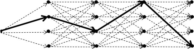
Figure 1.

Brownian bridges BBs, with one path of BBs in dark font. The times can be macroscopic.

How do we know a-priori where to send the BBs, e.g. where the OTM region is? Again recall the first step that runs a limited, although not too limited, MC simulation of SPs for which the pricing function is called. The SPs come back with enough information about “interesting” regions where substantial deal value exists. For step 2, we send BBs to those “interesting regions” [4].²

For further discussion, see Ref. [1], (Appendices 1–3).

2.4 Interpolated Brownian Bridges (IBB): third step

The third step is that we carry out interpolation for points sampled neither by SPs nor BBs. We term a path for which the interpolation takes place as an “interpolated Brownian Bridge” or IBB. This enables an effective “pricing” for all values of the underlying variables without calling the pricing function “too many times”.

Call x* a point at which we want to interpolate the deal with price C. We get C(x*) from the SP and BB values: $\left\{C\left({\mathit{x}}_{\mathit{b}}^{\left(\mathit{SP}\right)}\right)\right\}$, $\left\{C\left({\mathit{x}}_{\mathit{b}}^{\left(\mathit{BB}\right)}\right)\right\}$. To do this we need a distance measure and an interpolation function, discussed next.

2.4.1 Distance measure and interpolation function

Denote the square of the distance from point x_b to point x* as $d^2\left({\mathit{x}}^{\ast },{\mathit{x}}_{\mathit{b}}\right)={‖{\mathit{x}}^{\ast }-{\mathit{x}}_{\mathit{b}}‖}^2$ for a certain number of nearest SP, BB neighbors x_b with respect to x*. Based on some analysis, we preliminarily choose five nearest neighbors as the default. As the distance gets small, the number of nearest neighbors needs to decrease in order to reproduce the value at x*.

We choose a nearest-neighbor cutoff “Cauchy” interpolation weight using the squared distance function $d^2\left({\mathit{x}}^{\ast },{\mathit{x}}_{\mathit{b}}\right)$. The Cauchy distance bandwidth cutoff parameter $\kappa$ is used to control smoothness vs. variation.³

$$w\left({\mathit{x}}^{\ast },{\mathit{x}}_{\mathit{b}}\right)=\frac{{\left[d^2\left({\mathit{x}}^{\ast },{\mathit{x}}_{\mathit{b}}\right)+{\kappa }^2\right]}^{-1}}{\sum _{{\mathit{x}}_{\mathit{b}\text{'}}=5\text{nearest}\mathrm{nbs}\text{to}{\mathrm{x}}^{\ast }}{\left[d^2\left({\mathit{x}}^{\ast },{\mathit{x}}_{\mathit{b}}^{\text{'}}\right)+{\kappa }^2\right]}^{-1}}$$E1

2.4.2 Interpolated value of deal

The final interpolated value of the deal at x* is then

$$C_{\text{interp}}\left({\mathit{x}}^{\ast }\right)=\sum _{{\mathit{x}}_{\mathit{b}}=5\text{nearest}\mathrm{nbs}\text{to}{\mathit{x}}^{\ast }}C\left({\mathit{x}}_{\mathit{b}}\right)w\left({\mathit{x}}^{\ast },{\mathit{x}}_{\mathit{b}}\right)$$E2

3. SMC Stage 2: running the portfolio

3.1 Setup for portfolio run

The second stage for SMC simulation is a standard MC simulation. However, this second SMC stage never calls the pricing function, but rather uses the values of deals using the output of the three steps of the first SMC stage, namely price “look-up” tables that result from the prices from the SPs, BBs, and interpolation. Both stages constitute “Smart Monte Carlo”.

3.2 Full MC simulation of the SMC Stage 2

Consider a portfolio that consists of deals {C_l}. In Stage 1, we create the look-up tables for individual deals. Again, a look-up table lists the deal values produced from the interpolation for all points on a regular grid created in the space of the risk factors. Because the interpolation is conducted in a stepwise fashion, the number of look-up tables for the prices of a given deal equals the number of time steps in the simulation. The collection of the look-up tables provides the deal values on any path that has evolved arbitrarily. It is this feature that leads to substantial time saving in Stage 2 that only looks up deal values using the tables without either calling the pricer or doing the on-the-fly interpolations. Note that Stage 2 analysis does not need to compute the SMC probabilities. In a standard MC simulation, all paths are equally weighted with a total weight of 1.

The general procedure for the Stage 2 analysis consists of the following steps:

1. Run SMC Stage 1 analysis for each deal C_l. The SMC is customized for each type of deal using the strategies described above.

2. Create the SMC Stage 1 look-up tables for each deal {C_l}.

3. Generate standard MC paths for Stage 2.

4. Look up values for each deal along each MC path, which involves looking up through a table at each time in the time partition defining the MC simulator.

3.3 Deal/risk aggregation (Stage 2)

In Stage 2, the portfolio risks (expected values and PFEs - See Appendix) are calculated by aggregation—summing up the risks of individual deals for all MC paths. For each time step, a MC path provides all the necessary information in terms of the values of the underlying risk factors that are used to determine the deal values from the SMC look-up tables. Theoretically, there is no limit on the number of Stage 2 paths except for the possible constraint concerning the time for aggregating the deals. Deals with simple structures and complicated structures are treated in the same way. More importantly, the aggregation has no offset effect on the efficiency gained in the SMC Stage 1, in which SMC paths are customized to line up with the risk profiles of individual deals.

In summary the procedure is:

1. Aggregate the values/risks of all deals (portfolio) for all MC paths.

2. Calculate the portfolio expected values and PFE, or any other desired statistic, as in a conventional MC simulation.

4. Smart MC vs. standard MC: examples

4.1 OTM caps portfolio

The first illustrative example consists of 4 out-of-the-money OTM caps.⁴ This illustrates the ability of the SMC method to sample interesting regions more efficiently than standard MC (which only knows about the stochastic equations but not the financial instrument profile).⁵Figure 2 shows the results.

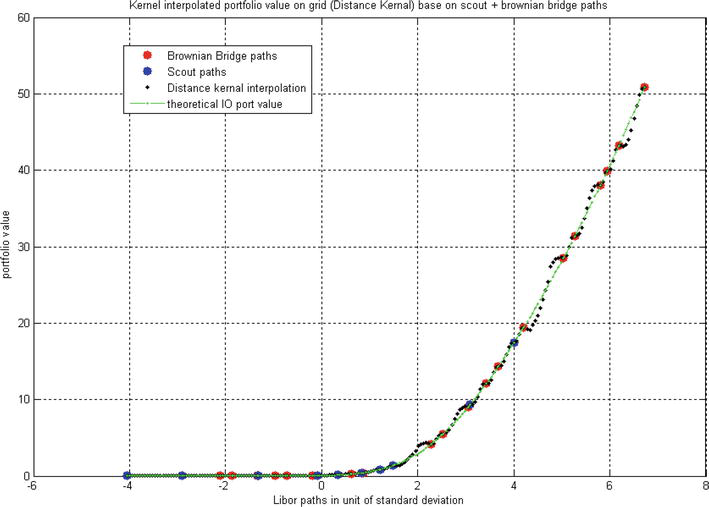
Figure 2.

Theoretical portfolio values and interpolated portfolio values from SPs (blue dots) and BBs (red dots), along with interpolated values (black dots), plotted vs. Libor in units of standard deviation, at three future times t_l (l = 1, 2, 3) years.

4.1.1 Smart MC results for OTM caps portfolio

The efficiency of the SMC “new method” using 10 SPs and 20 BBs (30 calls to each pricer) is demonstrated below. Tables 2 and 3 compare the expected values and the 90% PFEs for SMC against a conventional “regular” 100-path MC simulation (100 calls to each pricer). The uncertainty is estimated by doing the whole comparison procedure 10 times. The “true” portfolio value is defined using a large number of MC paths (10,000). See footnote 5 for more detail.

Expected value averaged over 10 simulations
	No. of paths/sim	C(t1)	C(t2)	C(t3)
Regular	100	2.1	2.1	1.2
New method	10 + 20 (intpl 200)	2.7	2.2	1.2
True	10,000	2.7	2.2	1.3

Standard deviation of expected value over 10 simulations
	No. of paths/sim	dC(t1)	dC(t2)	dC(t3)
Regular	100	0.14	0.14	0.14
New method	10 + 20 (intpl 200)	0.09	0.10	0.11
True	10,000	0.00	0.00	0.00

Table 2.

Expected value and error for OTM caps portfolio.

90% PFE averaged over 10 simulations
	No. of paths/sim	C(t1)	C(t2)	C(t3)
Regular	100	6.0	5.2	4.1
New method	10 + 20 (intpl 200)	6.6	6.5	3.9
True	10,000	6.7	6.2	3.8

Standard deviation of PFE over 10 simulations
	No. of paths/sim	dC(t1)	dC(t2)	dC(t3)
Regular	100	0.47	0.77	0.88
New method	10 + 20 (intpl 200)	0.25	0.35	0.46
True	10,000	0.00	0.00	0.00

Table 3.

PFE and error for OTM caps portfolio.

We thus cut down the number of evaluations by a factor of 3 using the SMC approach. We also get better results for values (expected and PFE) compared with the true value, along with smaller uncertainties (standard deviation).

4.2 Down and Out DO option with rebate

To test the Smart MC (SP + BB + IBB) method in the presence of a barrier, we use the classic down and out (DO) option along with a rebate paid at touch if the barrier is crossed.⁶ We get the expected value and the PFE at 90% CL.

The results are in Tables 4 and 5. The SMC method wins over a standard MC simulation by saving 1/2 of calls to the pricing function (50 for SMC from 30 SPs and 20 BBS, vs. 100 for standard MC) at each future time $t_{\mathrm{\ell }}$, $l=\mathrm{1...5}$.

Expected value averaged over 10 simulations
	No. of paths	C(t1)	C(t2)	C(t3)	C(t4)	C(t5)
Regular	100	15.1	14.0	14.6	14.0	13.5
New method	30 + 20 (intpl 200)	16.4	15.7	15.2	14.9	14.6
True	10,000	16.3	16.2	16.2	15.6	15.7

Standard deviation of expected value over 10 simulations
	No. paths/sim	dC(t1)	dC(t2)	dC(t3)	dC(t4)	dC(t5)
Regular	100	0.34	0.69	1.24	1.19	1.36
New method	30 + 20 (intpl 200)	0.08	0.04	0.02	0.03	0.05
True	10,000	0.00	0.00	0.00	0.00	0.00

Table 4.

Expected value and error for down and out option.

90% PFE averaged over 10 simulations
	No. of paths/sim	C(t1)	C(t2)	C(t3)	C(t4)	C(t5)
Regular	100	27.0	27.7	38.0	39.8	45.6
New method	30 + 20 (intpl 200)	29.6	36.2	41.4	46.9	50.9
True	10,000	28.6	34.9	39.9	43.6	51.3

Standard deviation of PFE over 10 simulations
	No. paths/sim	dC(t1)	dC(t2)	dC(t3)	dC(t4)	dC(t5)
Regular	100	1.28	0.95	2.65	2.65	7.81
New method	30 + 20 (intpl 200)	0.29	0.52	0.65	0.56	0.49
True	10,000	0.00	0.00	0.00	0.00	0.00

Table 5.

PFE and error for down and out option.

The down and out option addresses how we tackle the edge effect characterized by the difference of the option value above the barrier and the rebate below the barrier. Hence, the BBs need to be carefully positioned to separate these two states. This can easily be achieved by placing two BBs above and below the barrier with equal distance to the barrier, such that the bins around the BBs share a same edge at the barrier. Again, we are taking advantage of the discretion feature of the BBs that can be flexibly customized to either emphasize the interesting region or better classify the states.⁷

4.2.1 Smart MC results for DO option

4.3 Reconstruct the Matlab logo—2 dimensional example

In this section, we demonstrate the efficiency of the interpolation with a complicated “payout” function in two dimensions using the Matlab [5] Logo. The logo is the drawing of the leading eigenfunction of the wave equation with a “Pac-man” spatial geometry from the Matlab logo function, in Figure 3. Financial payoffs generally are less complicated, so this is a good test.

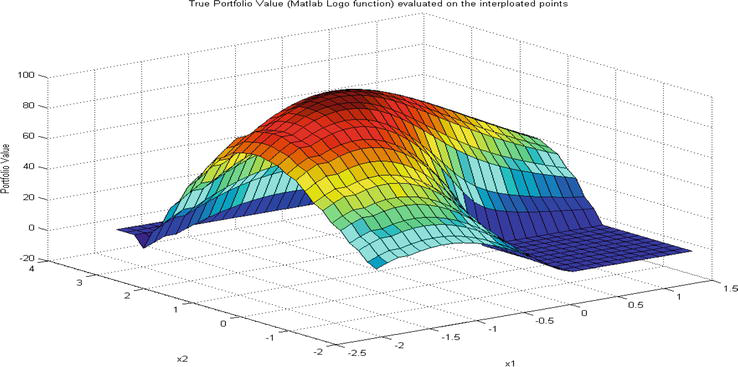
Figure 3.

The Matlab logo.

Figures 4–6 illustrate the stepwise results in the new method.⁸ We use 10 SPs (Figure 4) followed by 20 BBs (Figure 5). Here the Matlab logo from a “path” is really just a call to the Matlab logo function. With only 30 points in the 2 dimensional space calling the “pricing function” (i.e. the logo function) little resemblance is visible. Still, the interpolated result using the Cauchy distance kernel with five nearest neighbor points is fairly accurate (Figure 6). The SMC method Stage 1 with 30 calls to the Matlab logo function in the three steps gives a better reproduction of the Matlab logo than do the standard MC SPs with 100 calls to the Matlab logo function in Figure 7, a savings of at least a factor 3.

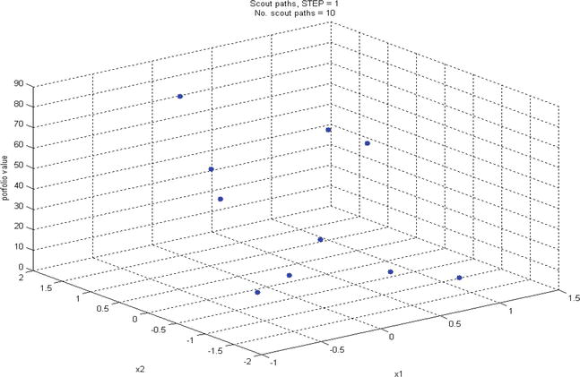
Figure 4.

The Matlab logo for the 10 SPs in SMC.

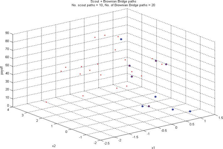
Figure 5.

The Matlab logo for the 20 BBs (red) and 10 SPs (Blue).

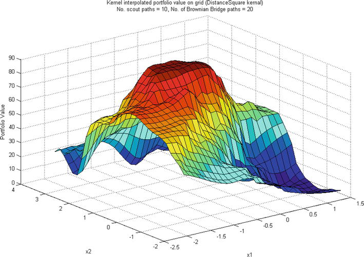
Figure 6.

The SMC interpolated result for the Matlab logo with the SP and BB input.

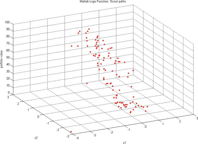
Figure 7.

Standard MC result for the Matlab logo with 100 paths.

Appendix: expected value and PFE with SMC

The expected value of a portfolio is the probability weighted average of the portfolio prices. In a standard MC simulation, the expected value is the same as the sample mean of the deal prices on the simulated paths which are generated based on the underlying variable distribution assumptions. However, in the path integral simulation, the expected value is the sum of the “interpolated Brownian Bridge” values multiplied by the corresponding bin probabilities. Here, for a given bin, the probability is the product of the path integral Green function from the initial point to the center of that bin, multiplied by the size of the bin (Ref. [3], Ch. 44). This is just a Riemann approximation to an ordinary calculus integral. We use a simple illustrative portfolio; the details are not important.

The red line in Figure 8 indicates the position of the expected value. The potential future exposure (PFE) in green is defined as the undiscounted portfolio value at a given future time calculated at some level of confidence, e.g. 90%. In the SMC simulation, the PFE procedure is⁹:

• Rank the IBBs for portfolio values from smallest to largest

• Compute the empirical cumulative distribution function CDF for the IBBs by sequentially adding the bin probabilities for the value-ordered IBBs

• The 90% PFE is the 10% = 1–90% percentile of the empirical CDF.

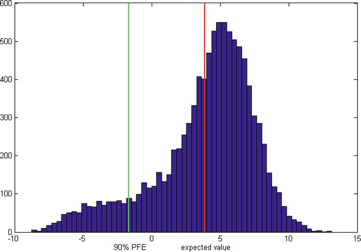
Figure 8.

Distribution (vertical axis) of simulated future illustrative portfolio values (horizontal axis); expected value (red), 90% CL PFE value (green).

Note

This paper was first published July, 2016 at SSRN (paper 2808177): https://ssrn.com/abstract=2808177 or http://dx.doi.org/10.2139/ssrn.2808177. Republished with permission from Bloomberg L.P. This work was created when the authors were employed at Bloomberg L.P.

References

- 1.
Dash JW, Yang X. Path Integrals and Smart Monte Carlo - II, Bloomberg L.P. working paper, 2016 (SSRN paper 2808179) - 2.
Dash JW, Yang X. Smart Monte Carlo, path integrals, and American options, Bloomberg L.P. working paper, 2016 (SSRN paper 2808186) - 3.
Dash JW. Quantitative Finance and Risk Management, A Physicist’s Approach. 2nd ed. Singapore: World Scientific Publishing Co. Pte. Ltd.; 2016. ISBN 978-981-4571-23-4. See chapters 41–45 - 4.
Atchadé YF, Rosenthal JS. On adaptive Markov chain Monte Carlo algorithms. Bernoulli. 2005; 11 :815-828 - 5.
Matlab, copyright The MathWorks, Inc.
Notes
- OTM means out of the money with respect to today’s price.
- Our BB construction is conceptually similar to some Metropolis-like filter that selects MC paths according to some criteria, with the criteria here depending on the financial instrument. Note that randomness still exists with a simple filter of MC paths; the method here is not a simple filter.
- We reduce the number of nearest neighbors when x* is close to one of the xb points. The number 5 of nearest neighbors for numerical applications here was determined empirically.
- The caps were taken as maturing in 4 years with strikes 50, 150, 250, and 350 bp respectively. The current Libor rate was taken as 40 bp, lognormal volatility constant at 15%.
- In Stage 1 of SMC, we use 10 SPs (step 1) and 20 BBs (step 2). Hence we call the pricing function 30 times for each cap at each time before maturity. The positions of the BB paths are determined algorithmically to emphasize the rate region in which the portfolio of OTM caps has a “substantial” non-zero payoff. For step 3, the SPs and BBs are the basis for the interpolator that estimates the value semi-parametrically, as a function of the underlying rate. That is, for any path not sampled by either SPs or BBs, the portfolio value is approximately determined without calling the pricing function. To this end, we position 200 IBBs that partition the rate space into 200 bins around the SPs and BBs. The portfolio values over the IBBs are obtained through the interpolation, and the path integral probabilities of 200 bins are computed offline.
- The option is taken as 5 year maturity, strike 100 and barrier 80. The rebate is 5% of notional paid into a bank account that accrues interest at 1%/year. The initial price is 100 with lognormal vol 15%.
- The probabilities attached to bins are computed differently for different states. For the bins above the barrier, the path integral probability is given by the product of the non-knock-out Green function (Ref. [3], Ch. 17) and the bin size in logarithmic scale. However, the bins below the barrier contain the paths being alive up to the previous step and knocked out at the current step. Hence, at step n, the probability is given by the product of the non-knock-out probability up to time step n − 1 and the knock-out probability over the time interval steps [n − 1, n]. This computation can be done either numerically or analytically. The former requires a numerical integration over the non-knock-out range at time step n − 1, which we used here.
- The “portfolio value” vertical axis is the height of the Matlab logo function above each point (x1, x2) in the plane.
- PFE measures the counterparty credit risk in the future during the lifetime of existing trades. In statistical terms, the 90% PFE is the 90% percentile of the distribution of forward portfolio values. For example in standard MC with 100 paths, the 90% PFE is given by the 10th smallest portfolio value since all paths are equally weighted.