Long Short-Term Memory Network Versus Support Vector Machine for Flood Prediction

Abstract

Malaysia is prone to flood disasters, which are considered the most hazardous natural disasters. This study compares the use of Long Short Term Memory (LSTM) networks and Support Vector Machines (SVM) in predicting future flash floods. Additionally, this study examines the effect of using the Synthetic Minority Oversampling Technique (SMOTE) in order to address imbalanced data. In this study, flooding for the year 2021 will be predicted based on the best-performing model. Experimental results indicated that the treatment had a positive impact on the study’s outcome. An analysis of the outcomes of the models before and after treatment was conducted in order to determine which model delivers a higher degree of accuracy. SVM with RBF kernel is the most effective model before and after SMOTE treatment, out of all those evaluated in the study. Next, SVM model using RBF kernel after treatment was used to forecast flooding for 2021. Seven out of 12 floods were predicted by the model, which equates to 58.33% accuracy. Since the deep learning model did not perform well, future researchers could experiment with different numbers of hidden layers and hyperparameter settings to increase the accuracy.

1. Introduction

Natural disasters, such as flooding, have become the most frequent natural hazard, posing a threat to people as well as their possessions. People living in the affected regions had to cope with this situation. Consequently, they were forced to relocate to safer locations offered by the government, such as public buildings, institutions, and religious buildings [1]. According to the World Meteorological Organization [2], flooding can be classified according to its preceding events. The types of floods include flash floods, fluvial floods, seasonal floods, urban floods, and snowmelt floods.

Known as torrential floods [3], flash floods are among the most prevalent natural disasters, causing extensive damage both in urban and rural areas [4]. Torrential floods are typically characterized by roaring torrents that ravage riverbanks, roads, and mountain valleys, sweeping away anything in their path. Heavy rains can cause torrential floods within minutes or hours. Due to its speed, torrential floods are difficult to predict. This gives people a limited amount of time to flee or to bring food and other essentials with them.

Flood disasters occur quite frequently in Malaysia and have been named the most dangerous natural disaster alongside landslides, tsunamis, hurricanes, and haze [5]. Malaysia’s Department of Irrigation and Drainage (DID) stated that flood prediction is intended to prepare an accurate and reliable forecast of imminent floods for citizens’ safety while simultaneously reducing risks and property damage [6, 7]. The frequency of heavy rainfall leading to flooding in the past is expected to increase due to weather pattern changes. As a result, it is vital to be able to predict future flood events in order to minimize the damage caused by floods.

There are several techniques that can be used to develop flood prediction models, including machine learning and deep learning [7, 8, 9]. A number of studies have been conducted on flood disaster management and flood prediction systems. The goal of machine learning, a subfield of computer science, is to make it possible for computers to “learn” without being explicitly taught. Machine learning “learns” through becoming more skilled at predictions, classifications, and clustering through “practice” [9, 10].

In the context of classification and regression prediction, SVMs entail using machine learning techniques in order to enhance predicted accuracy without overfitting the data. There is a wide range of applications for SVM, including hydrology and meteorology. The reasons for this are due to the fact that hydrological and meteorological data are nonlinear [11], concluded that SVM was more effective at forecasting rainfall than statistical or numerical approaches. A study conducted by Hasan et al. [12] predicted rainfall in Bangladesh with 99.92% accuracy using a Support Vector Regression (SVR) model and concluded that SVR is better than traditional approaches. However [13], claimed that SVM has certain limitations, and one of them is the fact that its accuracy is highly dependent on parameters and kernel functions.

LSTMs refer to Long-Short-Term Memory networks that are modified forms of Recurrent Neural Networks (RNNs). LSTMs are often used to learn order dependence in sequence prediction problems, particularly in time series data. As a result of its superiority in the field of prediction, LSTMs are widely used in the field of hydrology [10]. LSTM was tested for low-flow forecasting in the Mahanadi River basin in India [14], and the most accurate outcome was found to be achieved by LSTM. The study concluded that LSTM is the best modern method and acts as an accurate Artificial Intelligence (AI) technique, especially for low-flow forecasting [15], conducted a study that utilized LSTM models to forecast discharge at the Hoa Binh Station on the Da River. Using LSTM models in hydrology may offer the possibility of developing and managing real-time flood warning systems.

A flood danger rating prediction model was developed by Kim and Kim [16] utilizing LSTM modeling and random forest methods. LSTM neural networks were used by Fang et al. [17] to predict flood susceptibility by combining an appropriate engineering method with an LSTM model. For preventing and mitigating flood hazards, researchers may be inspired by the Local Spatial Sequential Long-Short-Term Memory (LSS-LSTM) approach. Additionally, LSTM models have been successfully used in a variety of flood-related applications, such as precipitation forecasts, rainfall-runoff models, and river flood forecasts [10]. Although LSTM has difficulty displaying specific peak values, it follows dominant patterns, which is critical for flood prediction. It has been reported that [9] has discovered that deep-learning techniques such as Recurrent Neural Networks (RNNs) and LSTMs are being utilized to develop flood predictions using deep-learning methods. As Artificial Intelligence (AI) technology develops, an LSTM network model might be well suited to address hydrological engineering challenges due to its ability to model large time-series data using deep learning techniques. It has been confirmed that deep-learning methods provide high levels of accuracy [14, 15, 16, 17].

In this study, we aim to develop supervised learning for flood prediction models based on the SVM algorithm and the LSTM network. The purpose of this study is to compare the accuracy of both models in predicting flooding in Subang Jaya. The SVM algorithm is a simpler prediction method, while LSTM networks are far more complicated. Understanding the pros and cons of each method will enable flood predictions to be made more accurately and efficiently in the future. This study could help future researchers choose between machine learning and deep learning when predicting upcoming floods.

2. Materials and methods

Explanation regarding data used in this project and the methods used to accomplish the objectives of this project are discussed in this section.

2.1 Data collection

Meteorological data alone especially using daily rainfall amount as the explanatory variable is seldom used to predict flooding, therefore there is not much info on flooding prediction using said data. The threshold of a variable is a crucial aspect when it comes to accuracies and precisely predicting flood. The city is in Peninsular Malaysia near Kuala Lumpur which is also susceptible to natural disasters such as flooding [18]. In this study, the meteorological dataset for the Subang Jaya area located at Sultan Abdul Aziz Shah Airport was obtained from the Malaysian Meteorological Department (MET Malaysia) located at Sultan Abdul Aziz Shah Airport. The data used in this project was 15 years’ worth of meteorological data for Subang Jaya starting from 1st January 2005 until 31st December 2020. There are 5844 observations and 8 variables in this dataset. These variables are year, month, day, daily maximum temperature (°C), daily minimum temperature (°C), daily relative humidity (%), daily rainfall amount (mm), and daily mean sea level (MSL) pressure (hPa). The unavailability of data regarding the previous flooding incidents in Subang station from 1st January 2005 to 31st December 2020 has become a challenge to check the accuracy of the prediction model. Hence, there is room for error when constructing the flood prediction model. Apart from the lack of meteorological data, deep learning, and machine learning have not been compared side-by-side for flood prediction models.

2.2 Feature engineering

Data cleansing, data normalization, data transformation, and feature creation are all part of feature engineering [19]. In this research, data cleansing was done where missing data, outliers, and duplicate values were checked. Following feature creation, two distinct variables are developed: “rain intensity”, as classified by Department of Meteorology, Malaysia in Table 1, and “flood occurrence”, as classified by MET Malaysia in Table 2. Afterward, the training data was normalized.

Category	Minimum rainfall (mm)	Maximum rainfall (mm)
Slight rain	0	10
Moderate rain	10	60
Heavy rain	60	150
Extreme rain	150	∞

Table 1.

Categories of rainfall intensity according to its range.

Rain intensity	Flood occurrence
Slight rain	No
Moderate rain	No
Heavy rain	Yes
Extreme rain	Yes

Table 2.

Classification of flood occurrence based on rain intensity.

2.3 Data splitting

The data were split into two parts: training and testing data. The number of observations used as a training set is 4383 datapoints, starting from 1st January 2005 to 31st December 2016. For the remaining 1460 data points from 1st January 2017 to 31st December 2020 were utilized as a testing set. The training set was used to develop the model, while the testing set was used to measure the model accuracy and then to forecast future rainfall values.

2.4 Data balancing

Imbalanced data refers to a situation where data samples in a problem are not distributed equally. As a result, one or more classes in the dataset are undervalued. The uneven distribution of data causes the algorithm unable to perform forecasts accurately in predicting minority groups, resulting in various classification mistakes. The Synthetic Minority Oversampling Technique (SMOTE) was implemented to remedy the unequal distribution of unbalanced data [20]. SMOTE is a procedure where interpolation among neighboring minority classes is done. Without simply just replicating the minority class, SMOTE creates synthetic data by finding k-closer neighboring data [10].

2.5 Support vector machine (SVM) algorithm

Machine learning algorithms’ expertise in data-driven learning rather than explicit teaching is also their main distinction from other computer programs. Numerous ML methods, such as Support Vector Machine (SVM), Naive Bayesian, and K-Nearest Neighbors (KNN) have proven to be crucial to support solutions in applications. SVM algorithm is a method of constructing a classifier that creates a decision boundary known as the hyperplane within the classes. Meanwhile, parameter tuning influences the classifier’s efficiency and effectiveness [21]. Among others, the kernel function selected can have a significant impact on SVM model performance. However, trial and error are the best methods for selecting the best kernel. The models can be constructed beginning with a simple SVM and then experimented with various “standard” kernel functions [22]. Table 3 shows the overall hyperparameters used in SVM models.

Kernel	γ	C	d	coef0
Linear	N/A	1	N/A	N/A
RBF	0.2	1	N/A	N/A
Polynomial	0.2	1	3	0
Sigmoid	0.2	1	N/A	0

Table 3.

Hyperparameters setting for SVM models.

*N/A stands for not applicable.

Apart from kernels, other hyperparameters used in the models are d = 3, γ = ‘0.2’, coef0 = 0, and C = 1 where all the values are default. The parameter ‘degree’ denoted as ‘d’ is often used when dealing with a polynomial kernel reflecting the flexibility of a decision boundary. The parameter ‘gamma’ denoted as γ is the radius area for misclassification and the parameter “coefficient” is denoted as ‘coef0’ significant only for polynomial and sigmoid kernel indicating the adjustable independent term in the kernel function. Finally, the parameter ‘C’ adds a certain penalty for any misclassification of an observation. Each kernel function has its equations represented as the following:

$$Linear:<x\text{,}{x}^{\prime }>$$E1

$$Polynomial:{\left(\gamma <x\text{,}{x}^{\prime }>+r\right)}^d$$E2

$$RBF:\exp {\left(-\gamma \text{||}x\text{,}{x}^{\prime }\text{||}+r\right)}^d$$E3

$$Sigmoid:\tanh \left(\gamma <x\text{,}{x}^{\prime }>+r\right)$$E4

2.6 Long short-term memory (LSTM) network

The primary feature of an LSTM network is the hidden layer named as memory cells which has three gates named $forgetgate\left(f_t\right),$ $inputgate\left(i_t\right),$ and $outputgate\left(O_t\right)$. $f_t$ gates are responsible for making decisions regarding what information is to be removed from the cell state. $i_t$ gate is to specify what information ads to the cell state. $O_t$ is to specify what information that was used from the cell state. The LSTM network has three major layers which are an input layer, single or multiple memory cells, and an output layer. The number of neurons in the input layer is equivalent to the number of the variables, in this would be 5. More layers require more computational time so, this project uses only two layers.

A memory cell starts functioning by removing information from the previous cell state, $S_{t-1}$ are determined by the LSTM layer. At time stamp t, the activation value $f_t$ of the forget gates is calculated using the existing input, $x_t$ and output, $h_{t-1}$ of the memory cells at $t-1$ and the bias terms of forgetting gates, $b_f$. The sigmoid function adjusts all activation levels to 0 and 1 as entirely forgotten and completely recalled, respectively. Secondly, the LSTM layer would determine the information that was included in the network’s cell states, $S_t$. This computes the candidate’s values, $\widetilde{S_t}$ and then activation values of the input gates. Thirdly, where new cell states, $S_t$ are calculated using the information of the preceding 2 steps. Finally, the output, $h_t$ of the memory cells unit is acquired. The hyperparameters used in this typical LSTM model include certain functions with default values and are listed in Table 4 [23]. The activation function enables the model to undergo non-linear processes.

Hyperparameter	Value
Number of hidden layer	2
Activation	Hyperbolic tangent (tanh)
Recurrent_activation	sigmoid
Epoch	100 or 200
Batch size	64
Dropout	0.2
Optimizer	Stochastic Gradient Descent method (Adam)
Loss	binary_crossentropy

Table 4.

Hyperparameter setting for LSTM (2) model.

Recurrent_activation is used for the recurrent step and optimizer is used to reduce the overall loss and improve accuracy. The optimizer used for this model is the stochastic gradient descent method known as ‘Adam’ which is based on adaptive estimation of first-order and second-order moments. Loss identifies if the prediction is good (low loss value) or bad (high loss value).

2.7 Confusion matrix, receiver operating characteristics (ROC) curve and area under the curve (AUC) value

To evaluate the performance of the models, the confusion matrix was constructed since it provided information such as accuracy, precision, recall, F1-Score, and the AUC for the ROC curve [24]. Table 5 shows the framework for a confusion matrix.

		Actual class
		Positive	Negative
Predicted class	Positive	True Positive	False Positive
	Negative	False negative	True negative

Table 5.

Confusion matrix.

The equations used to calculate the Precision, Recall, F1-Score, Accuracy, and Area Under the Curve (AUC) values are as follows:

$$Accuracy:A=\frac{TP+TN}{TP+FP+TN+FN}$$E5

$$Precision:P=\frac{TP}{TP+FP}$$E6

$$Recall:R=\frac{TP}{TP+FN}$$E7

$$F\_1-score:F=\frac{\left(2\ast P\ast R\right)}{\left(P+R\right)}$$E8

$$AUC=\frac{\sum TP+\sum TN}{\left(P+N\right)}$$E9

3. Results and discussion

Data analysis of the output from the experiments is shown in this section. The results from the models constructed discussion and analyzed by using the confusion matrix, ROC curve, and AUC. This section also discusses the objectives of this research.

3.1 Feature engineering

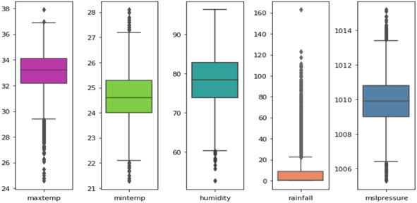
There are a number of steps discussed under this subtopic, including handling missing data, checking for outliers, creating features, and normalizing data. The column daily relative humidity has 10 missing values. As the number of missing values was less than 5%, they are not considered significant. Therefore, imputation was performed by replacing missing values with the mean of the column daily relative humidity (%), which is 78.13. Apart from missing values, no duplicate dates were found for this dataset. Figure 1 shows a boxplot constructed to check for outliers. The maximum temperature, humidity, and rainfall are the only three variables that exhibit outliers. Meanwhile, the minimum temperature has a slight negative skewness.

Figure 1.

Boxplot for each variable.

Next, variables minimum temperature and rainfall are skewed positively. Both, variables humidity and MSL pressure on the other hand show normal distributions. Since coming across an extreme value is common for meteorological data, it is determined that outliers are normal to exist and should not be removed [25]. After cleaning the data, feature creation was done where two new variables were created using daily rainfall amount. The variables created were based on information in Tables 1 and 2 as viewed in Section 2. Normalizing data is an important part of data pre-processing to ensure that the scale has been changed without distorting the information of an observation. In this research, the dataset was normalized in the range 0 to 1. This maintains the general distribution of the observation but simply converts the data to improve performance and accuracy.

3.2 Data balancing

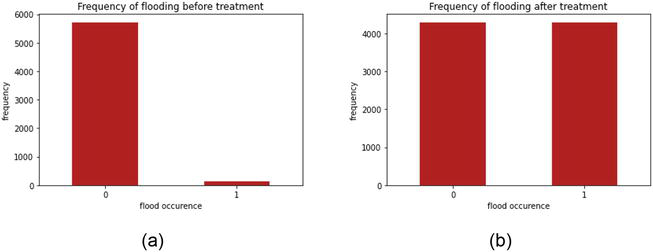
Without treatment, the accuracy and precision value might seem, high, however, the prediction is fundamentally biased in the sense of the representation of classes. Figure 2(a) shows the frequency of classes before treatment. The bar chart shows that the classes are severely imbalanced and would require treatment to ensure unbiased predictions. “1” is denoted as “flooding” and “0” is denoted as “no flooding,” Figure 2(b) shows the bar chart after the treatment. The classes are balanced where more “1” is predicted by producing synthetic data using SMOTE. Prediction models using both before and after treatment are done for both machine and deep learning methods and the difference of accuracy is shown.

Figure 2.

(a-b) Bar chart of balance of class for flood occurrences before and after treatment.

3.3 Support vector machine (SVM)

The SVM algorithm was used to construct a total of 4 models before and after treatment, respectively. This is because each model is constructed using different hyperparameter settings. By constructing the models using the suitable hyperparameter settings, the outputs were obtained. Table 6 shows the results from the confusion matrix for all SVM models using different hyperparameter settings before and after treatment. According to Table 6, SVM models using linear kernels has performed very well, however, the perfect results using linear kernel exhibits signs of overfitting. Overfitting models are highly prone to provide misleading results.

Kernel	Treatment	Precision	Recall	F1-score	Accuracy	AUC
Linear	After	1.0000	1.0000	1.0000	1.0000	1.0000
	Before	1.0000	1.0000	1.0000	1.0000	1.0000
RBF	After	0.9758	0.8790	0.9217	0.9945	0.8790
	Before	0.9480	0.6721	0.7465	0.9863	0.6721
Polynomial	After	0.6908	0. 9836	0. 7678	0.9678	0.9836
	Before	0.9911	0.5517	0.5892	0.9822	0.5517
Sigmoid	After	0.0099	0.5000	0.0195	0.0199	0.5000
	Before	0.4901	0.5000	0.4950	0.9801	0.5000

Table 6.

SVM results for different hyperparameter settings before and after treatment.

*Bold values indicate best-performing model.

Furthermore, the experiments showed that SVM with RBF have the most feasible results for both before and after SMOTE treatment. Before treatment, the AUC value is 0.6721 and the accuracy is 0.9863 meanwhile after the treatment, the AUC value increases to 0.8790 and the accuracy to 0.9945. SVM with RBF also showed stability in terms of statistical performance measurements, compared to other kernel functions.

Table 7 shows the percentage of improvement for SVM with RBF kernel after SMOTE treatment. Detailed analysis showed the precision improved by 2.85% from 0.9480 to 0.9758 and accuracy has improved from 0.6721 to 0.8790 which is 23.54%. Overall, all statistical performance measurement exhibit an increased performance after SMOTE treatment.

Evaluation metrics	Before treatment	After treatment	Percentage of improvement (%)
Precision	0.9480	0.9758	2.85
Recall	0.6721	0.8790	23.54
F1-Score	0.7465	0.9217	19.01
Accuracy	0.9863	0.9945	0.82
AUC	0.6721	0. 8790	23.54

Table 7.

Percentage of improvement SVM models using RBF kernels before and after treatment.

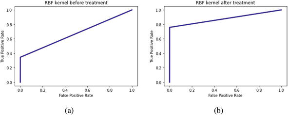
When it comes to ROC curve, a steeper curve indicates a better-performing model. Figure 3(a-b) shows ROC curves of SVM models each using RBF kernel and its specified hyperparameter settings before and after treatment which exhibits that the best performing kernel is the RBF kernel since there is no overfitting yet feasible result. Figure 3(a) reveals a moderately performing ROC curve with AUC value of 0.6721. However, there is still room for improvement in terms of the accuracy of the models. Figure 3(b) shows the ROC curves that performed better, and the ROC curve has a value of 0.8790 which supports the claim that treatment for SVM algorithm of RBF kernel is the best model.

Figure 3.

(a-b) ROC Curve for SVM algorithm RBF kernel before and after treatment.

3.4 Long short-term memory (LSTM) network

This research utilizes an LSTM network with a total of 4 layers constituting 1 input layer, 2 hidden layers, and 1 output layer. The input and hidden layers have 5 nodes each and the output layer has 1 node. This can be changed accordingly through trial and error. A summary of the output obtained from the confusion matrices is in Table 8. The best-performing model according to Table 8 is LSTM with 100 epochs before treatment due to the highest AUC value that is feasible.

Epoch	Treatment	Precision	Recall	F1-score	Accuracy	AUC
Epoch = 100	After	0.6169	0. 9668	0. 6724	0.9349	0.9668
	Before	0.7640	0. 9571	0. 8329	0.9822	0.9571
Epoch = 200	After	0.6466	0.9266	0.7106	0.9555	0.9752
	Before	0.7290	0.9040	0.7905	0.9774	0.9195

Table 8.

LSTM results for different hyperparameter settings before and after treatment.

Table 9 was constructed to better view the percentage of improvement for best best-performing LSTM model before and after treatment. Table 9 proves to apply treatment of SMOTE to the LSTM of epoch 100 prediction model has decreased its prediction ability. The precision of model has decreased by 23.85% from 0.7640 to 0.6169 and the accuracy has decreased from 0.9822 to 0.9349 which is a 5.06% deterioration. Finally, the AUC has increased slightly (1.00%) from 0.9571 to 0.9668. Overall, treatment has not shown much difference for the model.

Evaluation metrics	Before treatment	After treatment	Percentage of improvement (%)
Precision	0.7640	0.6169	−23.85
Recall	0.9571	0.9668	1.00
F1-Score	0.8329	0.6724	−23.87
Accuracy	0.9822	0.9349	−5.06
AUC	0.9571	0. 9668	1.00

Table 9.

Percentage of improvement LSTM model for 100 epochs before and after treatment.

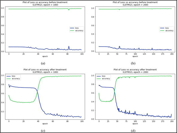
Figure 4(a) and (b) show the plot of loss versus accuracy for the constructed LSTM (2) networks before and after treatment. Figure 5(a) and (b) shows the plot have accuracy and loss that are a good fit continuously likely leading to an overfit. Figure 5(c) and (d) shows the loss and accuracy converged to a certain epoch value and diverged to maximum value meaning the models had trained well for the dataset and produced relatively high accuracy.

Figure 4.

(a-d) Plot loss vs. accuracy for LSTM of different epochs before and after treatment.

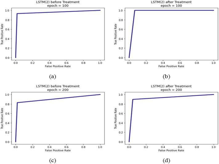
Figure 5.

(a-d) ROC for LSTM of different epochs before and after treatment.

3.5 Forecasting flood for year 2021

The best-performing model has been chosen as the SVM algorithm model utilizing the RBF kernel after treatment since it has a higher precision and accuracy which is 0.9758 and 0.9945 respectively compared to LSTM of 100 epochs after treatment which has a precision and accuracy of 0.6169 and 0.9349 respectively. Since the best model is determined as SVM model of RBF kernel after treatment, the forecasting of flooding was done using raw meteorological data for the year 2021. The expected output was Subang Jaya should have experienced flooding for a total of 12 days in the year 2021. However, the outcome was that Subang Jaya experienced 7 days of flooding only. The ratio of outcome to expected outcome is 7:12 which is approximately 58.33%. The model failed to predict flooding 41.67% of the times. This might be due to certain factors such as temperature, humidity, and MSL pressure fluctuations that were not detected by the model.

Figure 5 shows the ROC curves for LSTM models of respective hyperparameter settings before and after treatment is given. All ROC curves for the LSTM model of different epochs have performed well. However, the best-performing model is LSTM of epoch 100 after treatment since the ROC curve is steep and almost reaches the upper left corner of the graph. This claim is supported by the AUC value of 0.9668 proving that LSTM of 100 epoch after treatment performed the best.

4. Conclusion

To conclude, the SVM model with RBF kernel, γ = ‘0.2,’ and C = 1 after treatment would be the appropriate choice to construct a future flood prediction model based on meteorological data for the Subang Jaya area. This is because SVM models require lesser computational time and are easier to compute compared to LSTM networks since SVM algorithms do not need multiple layers. Besides, the accuracy for the SVM model using RBF kernel after treatment is 0.9945 which is exceptionally good. Using SMOTE as a treatment for imbalanced data has also shown significantly better accuracy in the models. The findings from this study indicate that SVM is better compared to LSTM. Due to the fact that SVM models require less computational time and are simpler to compute than LSTM networks. SVM algorithms do not require multiple layers of computation. Additionally, the accuracy of the SVM model using RBF kernel after treatment is 0.9945, which is exceptionally high. The use of SMOTE as a treatment for imbalanced data has also demonstrated a significant improvement in the accuracy of the models.

Future researchers will be able to take into account the computational time and complexity of the model when predicting flooding using meteorological data. The positive impact of using SMOTE in this research will also assist researchers in developing a better flood prediction model in the future, preventing biased results from occurring. To improve the accuracy of the models, future researchers may utilize different values of hyperparameters. It would be possible to produce a better prediction using LSTM network by adding more hidden layers and nodes within the layers. More hidden layers and nodes might help the neural network to learn more features and predict accurately. Higher epochs and batch size might also help increase the accuracy of a neural network. As for the SVM models, more hyperparameters could be explored to produce better predictions.

Acknowledgments

This research was supported by research grant FRGS/1/2022/ICT06/UTHM/03/1 provided by the Ministry of Higher Education, Malaysia. The authors would also like to thank the Faculty of Applied Sciences and Technology, Universiti Tun Hussein Onn Malaysia for its support.

Conflict of interest

The authors declare no conflict of interest.

Data availability statement

Data is deemed private and confidential and will not be shared.

References

1.Saimi FM, Hamzah FM, Toriman ME, Jaafar O, Tajudin H. Trend and linearity analysis of meteorological parameters in peninsular Malaysia. Sustainability. 2020;12(22):9533-9552
2.World Meteorological Organization. Manual on Flood Forecasting and Warning. Switzerland: Publications Board World Meteorological Organization (WMO); 2020
3.Bi Q , Goodman KE, Kaminsky J, Lessler J. What is machine learning? A primer for the epidemiologist. American Journal of Epidemiology. 2019;188(12):2222-2239
4.Syeed MMA, Farzana M, Namir I, Ishrar I, Nushra MH, Rahman T. Flood prediction using machine learning models. In: 2022 International Congress on Human-Computer Interaction, Optimization and Robotic Application (HORA). 2022. pp. 1-6
5.Adib M, Razi M, Tahir W, Alias N, Ismail LH, Ariffin J. Development of rainfall model using meteorological data for hydrological use. International Journal of Integrated Engineering. 2013;5(1):64-73
6.Department of Irrigation and Drainage. National Flood Forecasting and Warning Centre. 2022. Available from: https://www.water.gov.my/index.php/pages/view/195 [Accessed: May 15, 2022]
7.Mosavi A, Ozturk P, Chau KW. Flood prediction using machine learning models: Literature review. Water (Switzerland). 2018;10(11):1536-1548
8.Faruq A, Arsa HP, Hussein SFM, Razali CMC, Marto A, Abdullah SS. Deep learning-based forecast and warning of floods in Klang River, Malaysia. Ingenierie Des Systemes d’Information. 2020;25(3):365-370
9.Moishin M, Deo RC, Prasad R, Raj N, Abdulla S. Designing deep-based learning flood forecast model with ConvLSTM hybrid algorithm. IEEE Access. 2021;9:50982-50993
10.Kratzert F, Klotz D, Brenner C, Schulz K, Herrnegger M. Rainfall- runoff modelling using long short-term memory (LSTM) networks. Hydrology and Earth System Sciences. 2018;22(11):6005-6022
11.Hirani D, Mishra N. A survey on rainfall prediction techniques. International Journal of Computer Application. 2016;6(2):28-42
12.Hasan N, Nath NC, Rasel RI. A support vector regression model for forecasting rainfall. In: 2nd International Conference on Electrical Information and Communications Technologies (EICT). 2015. pp. 554-559
13.Zhang J, Qiu X, Li X, Huang Z, Wu M, Dong Y. Support vector machine weather prediction technology based on the improved quantum optimization algorithm. Computational Intelligence Neuroscience. 2021:1-13. DOI: 10.1155/2021/6653659
14.Sahoo BB, Jha R, Singh A, Kumar D. Long short-term memory (LSTM) recurrent neural network for low - Flow hydrological time series forecasting. Acta Geophysica. 2019;67(5):1471-1431. DOI: 10.1007/s11600-019-00330-1
15.Le X, Ho H. V, Lee G, Jung S. Application of long short-term memory (LSTM) neural network for flood forecasting. Water. 2019;11(7):1387
16.Kim HI, Kim BH. Flood Hazard rating prediction for urban areas using random Forest and LSTM. KSCE Journal of Civil Engineering. 2020;24(12):3884-3896. DOI: 10.1007/s12205-020-0951-z
17.Fang Z, Wang Y, Peng L, Hong H. Predicting flood susceptibility using LSTM neural networks. Journal of Hydrology. 2021;594:125734. DOI: 10.1016/j.jhydrol.2020.125734
18.Rahman IA, Dewsbury J. Selection of typical weather data (test reference years) for Subang, Malaysia. Building and Environment. 2007;42(10):3636-3641
19.Bekar ET, Nyqvist P, Skoogh A. An intelligent approach for data pre-processing and analysis in predictive maintenance with an industrial case study. Advances in Mechanical Engineering. 2020;12(5):1-14
20.Asniar, Maulidevi NU, Surendro K. SMOTE-LOF for noise identification in imbalanced data classification. Journal of King Saud University - Computer and Information Sciences. 2021;34(6):3413-3423
21.Ramasamy LK, Kadry S, Nam Y, Meqdad MN. Performance analysis of sentiments in twitter dataset using SVM models. International Journal of Electrical and Computer Engineering. 2021;11(3):2275-2284
22.Huang S, Nianguang CAI, Penzuti Pacheco P, Narandes S, Wang Y, Wayne XU. Applications of support vector machine (SVM) learning in cancer genomics. In Cancer Genomics and Proteomics. 2018;15(1):41-51
23.Team, K. Keras Documentation: LSTM layer. Keras.io. 2023. Available from: https://keras.io/api/layers/recurrent_layers/lstm/. [Accessed: January 11, 2023]
24.Sellami EM, Maanan M, Rhinane H. Performance of machine learning algorithms for mapping and forecasting of flash flood susceptibility in Tetouan, Morocco. The International Archives of the Photogrammetry, Remote Sensing and Spatial Information Sciences. 2021;2022(4):305-313
25.Zhang AZ, Li JZ, Gao H, Chen YB, Ma HZ, Bah MJ. CrowdOLA: Online aggregation on duplicate data powered by crowdsourcing. Journal of Computer Science and Technology. 2018;33(2):366-379
Written By
Hema Varssini Segar, Puteri Natasha Sofia Zulkafli and Shuhaida Ismail
Submitted: 26 June 2023Reviewed: 10 October 2023Published: 21 February 2024