Perspective Chapter: Frequency Domain Models of Nonlinear Loads in Power Systems

Abstract

Section 1 deals with harmonic current sources models for one diode and two diodes rectifiers, the model parameters being determined by simulations. Section 2 describes frequency domain (FD) models of nonlinear home appliances whose parameters are determined by measurements. Some FD models for the loads using firing angle control devices are presented in Section 3. The fourth section presents the simulations of a relatively large circuit in the time domain (TD) and in the FD using the algorithms of CADENCE and ADS. The HB analysis of ADS using the proposed FD models proves to be the most efficient for this example.

1. Introduction

Although AC networks contain only undistorted sinusoidal sources of the same frequency f, their actual voltages and currents often have other spectral components including several odd and sometimes even multiples of f. The presence of these spectral components (called harmonics) is due to nonlinear loads such as arcing devices, saturated transformers, and various types of rectifiers that power electric transport vehicles or electronic equipment.

The additional losses caused by current harmonics can be reduced by complementary power compensation. In order to bring the harmonic pollution in the power grid to an acceptable level [1], some iterative algorithms are used to design the compensation circuit or to determine its optimal size and location to minimize the effects of harmonics [2]. This type of calculation sometimes uses evolutionary algorithms, the efficiency of which depends on the effectiveness of the variant analysis of nonlinear energy systems.

Usually, periodic steady-state computation of nonlinear power systems is performed by the time domain analysis. Some transient analysis programs such as EMTP (Electromagnetic Transient Program) or EMTDC (Electromagnetic Transient Design and Control) use the “brute force” approach (integrating circuit equations until all transients decay) to achieve this [3, 4]. This method is not efficient for circuits with time constants much larger than the signal period. In this case, is preferred the shooting method using the Newton-Raphson algorithm [4].

Another method for calculating the periodic steady state of nonlinear circuits is the frequency domain analysis. The best method of this kind is the harmonic balance (HB) algorithm, which works on both frequency domain and time domain representations of the same signal [4, 5]. A signal is represented in the time domain by a set of evenly spaced samples, while in the frequency domain by a set of spectral components. These two sets are related by the direct discrete Fourier transform and inverse discrete Fourier transform, so the results of time domain analysis can be easily transformed to the frequency domain, and the results of frequency domain analysis can also be transformed to the time domain [5].

2. Current sources models with parameters determined by simulations

2.1 One diode rectifier

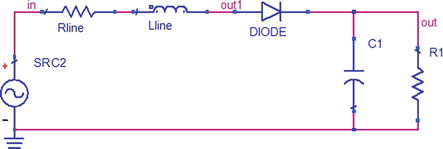
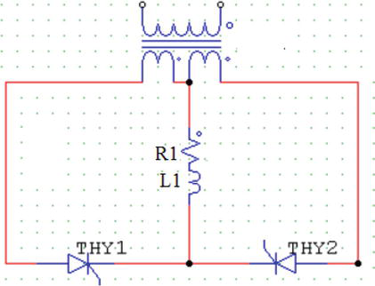
The circuit in Figure 1 is driven by a sinusoidal voltage source with amplitude V = 220 V and f = 50 Hz, having C₁ = 2 mF and R₁ = 37 Ω. The rectifier is connected to the AC source by a cable of 10mm², with a length of 30 m (R_line = 0.1104 Ω, L_line = 72 μH).

Figure 1.

One diode rectifier with a C filter.

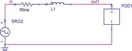
Starting from the linear dependence of the current harmonics amplitudes and phases on the amplitude and phase on the input voltage fundamental component suggested in Ref. [3] and using the simplified rectifier schematic described in Refs. [6, 7], the model of the frequency-defined device (FDD) in Figure 2 has been built. This model is described by a linear-controlled current source for each harmonic component, the control parameters being the amplitude and the phase of the voltage fundamental component V₁.

Figure 2.

Linear-controlled source model for the circuit in Figure 1.

This model is given in Figure 2, followed by its ADS description [8].

V₁ = V(out1)

I₀ = polar(1.7e-2*mag(V₁), 0)

I₁ = polar(3.14e-2*mag(V₁), 5 + 1*phase(V₁))

I₂ = polar(2.45e-2*mag(V₁), 11 + 2*phase(V₁))

I₃ = polar(1.54e-2*mag(V₁), 17 + 3*phase(V₁))

I₄ = polar(6.72e-3*mag(V₁), 25 + 4*phase(V₁))

I₅ = polar(6.83e-4*mag(V₁), 73 + 5*phase(V₁))

I₆ = polar(2.48e-3*mag(V₁), −158 + 6*phase(V₁))

I₇ = polar(2.53e-3*mag(V₁), −147 + 7*phase(V₁))

I₈ = polar(1.07e-3*mag(V₁), −134 + 8*phase(V₁))

I₉ = polar(5.059e-4*mag(V₁), 21 + 9*phase(V₁))

I₁₀ = polar(1.145e-3*mag(V₁), 41 + 9*phase(V₁))

The coefficients in the amplitude and phase description of the current harmonics are identified by simulations of the circuit in Figure 1.

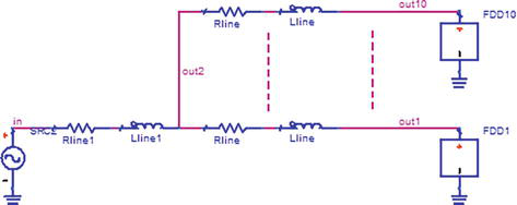
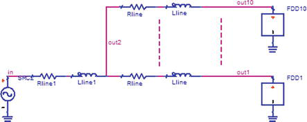
A test circuit consisting of 10 identical one-diode rectifiers, connected to a sinusoidal source with f = 50 Hz and amplitude V = 220 V through a 50 mm² cable of 30 m (Figure 3) has been used for the harmonic balance analysis, where R_line1 = 34.8 mΩ and L_line1 = 57.6 μH.

Figure 3.

One-phase test circuit.

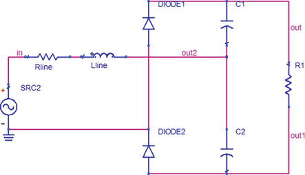
2.2 Two diode rectifier

A similar model can be made for a two diode rectifier (Figure 4). This circuit represents a reduced model of a compact fluorescent lamp [6, 7]. The parameter values are C₁ = C₂ = 15 μF, R₁ = 5 kΩ.

Figure 4.

Two diode rectifier.

In this case, the line is a 1 mm² cable with a length of 30 m, Rline = 1.08 Ω, and Lline = 72 μH. This model is described as follows [8]:

V₁ = V(out2)

I₁ = polar(1.276e-3*mag(V₁), 31 + 1*phase(V₁))

I₃ = polar(1.024e-3*mag(V₁), 94 + 3*phase(V₁))

I₅ = polar(6.453e-4*mag(V₁), 164 + 5*phase(V₁))

I₇ = polar(3.394e-4*mag(V₁), −105 + 7*phase(V₁))

I₉ = polar(2.643e-4*mag(V₁), 9 + 9*phase(V₁))

I₁₁ = polar(2.501e-4*mag(V₁), 101 + 11*phase(V₁))

I₁₃ = polar(1.924e-4*mag(V₁), −165 + 13*phase(V₁))

I₁₅ = polar(1.5961e-4*mag(V₁), −60 + 15*phase(V₁))

I₁₇ = polar(1.532e-4*mag(V₁), 38 + 17*phase(V₁))

I₁₉ = polar(1.3174e-4*mag(V₁), 133 + 19*phase(V₁))

I₂₁ = polar(1.161e-4*mag(V₁), −124 + 21*phase(V₁))

The test circuit similar to the one in Figure 3, where 10 identical two diode rectifiers are connected to a sinusoidal source with f = 50 Hz and amplitude V = 220 V through a 10 mm² cable of 30 m has been used for the harmonic balance analysis, where R_line1 = 110.4 mΩ, L_line1 = 72 μH.

2.3 Analysis

The test circuit of 10 identical one-diode rectifiers, connected to a sinusoidal source of f = 50 Hz and amplitude V = 220 V through a 50 mm² cable of 30 m with R_line1 = 0.0348 Ω, L_line1 = 57.6 μH, (Figure 5) has been used for the harmonic balance analysis [6].

Figure 5.

One-phase test circuit.

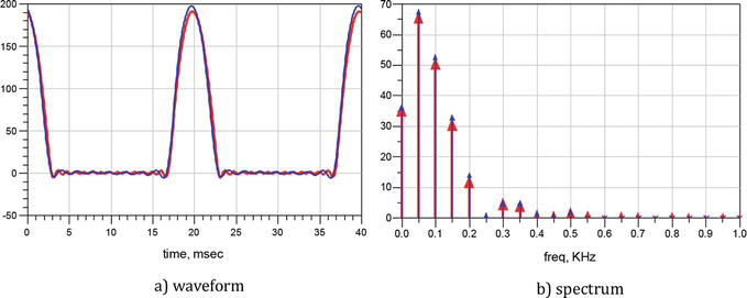
This section presents the results of a harmonic balance analysis performed using ADS. Two circuits with the structure shown in Figure 5 are analyzed. The current through the sinusoidal voltage source can be considered as a global variable representing the behavior of the test circuit. Results shown as red waveforms or spectral lines are obtained using a classical nonlinear model defined by time domain eqs. (TD model). Results shown as blue waveforms or spectral lines were determined using the models described in Sections 1.1 and 1.2.

The current through the sinusoidal voltage source can be viewed as a global variable representing the behavior of the test circuit (Figure 6) [8].

Figure 6.

Source current for the circuit in Figure 5 with one diode rectifier: (a) waveform and (b) spectrum.

The results obtained using the classical time-domain model are similar to those obtained using the proposed model, in the both time and frequency domains. The analysis using the classical time-domain model takes 0.96 seconds, while the analysis using the proposed model takes only 0.17 seconds. In both cases, 20 significant harmonic components are considered.

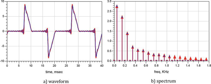
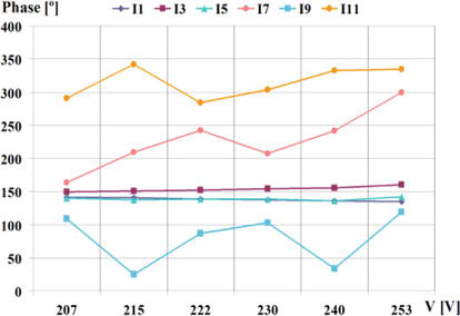
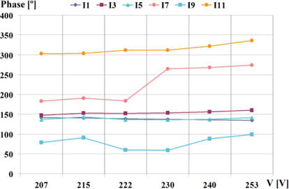
The harmonic balance analysis of a test circuit of 10 two-diode rectifiers produced similar results (Figure 7). In this case, the simulation time is 4.12 seconds using the classical nonlinear model described in the time domain, but only 0.19 seconds using the proposed model.

Figure 7.

Source current waveform for the circuit in Figure 5 with two diode rectifiers: (a) waveform and (b) spectrum.

These simulations have been performed with 35 harmonic components. It is obvious that as the harmonics number increases, a greater simulation time is obtained using FD models.

Some other properties of these FD models are described in Ref. [8]: It can reproduce the third current harmonic reduction as the length of a line supplying fluorescent lamps increases [6]. The accuracy of this simple model is not preserved for long lines of about several Km.

The proposed FD model reduces the simulation time by about an order of magnitude compared to the classical TD model using nonlinear loads described in the time domain. This result can be explained as follows:

• using the proposed model, the harmonic balance works only in the frequency domain, whereas using the classical model with nonlinear components, the algorithm works in both the frequency and time domains,

• no source stepping is required when using the proposed model, unlike when using the TD model in the same circuit.

The content of the paragraph “1. Current sources models with parameters determined by simulations” reproduces the research reported for the first time in Ref. [8].

3. Current source models with parameters determined by measurements

Numerous home appliances have complex electronic circuits, and in some cases, circuit diagrams and/or unknown parameters are not available and the methods in Section 1 cannot be used. A new approach to computing the parameters of their FD models, based on measurements, is described in this section [9, 10].

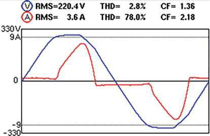
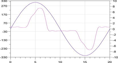
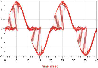
An analyzer is a relatively simple apparatus able to compute the modules and phases of the harmonic components of a non-sinusoidal waveform; the results are given with two significant digits. For example, an air conditioning system whose voltage and current waveforms are given in Figure 8 has its measured current harmonic components given in Table 1. Considering these harmonic components, the waveform in Figure 9 is rebuilt. This waveform is, at first glance, very close to that in Figure 8. Similar FD models have been built for a vacuum cleaner, a microwave oven, and a compact fluorescent lamp [8]. A three-phase network containing the FD models mentioned before has been simulated with the usual TD models and with proposed FD models. Because of the low precision of the measurements made with the analyzer (1–3 digits), the results obtained with these FD models are not accurate.

Figure 8.

Air conditioning system voltage and current waveforms—Measurements.

H order	1	3	5	7	9	11	13	15	17	19
I [A]	2.8	1.9	0.75	0.3	0.3	0.1	0.1	0.1	0.1	0.1
Phase [°]	0	147	−70	2	126	−120	−80	55	110	−140

Table 1.

Air conditioning system measured current harmonic components.

Figure 9.

Air conditioning system voltage and current waveforms—Simulation.

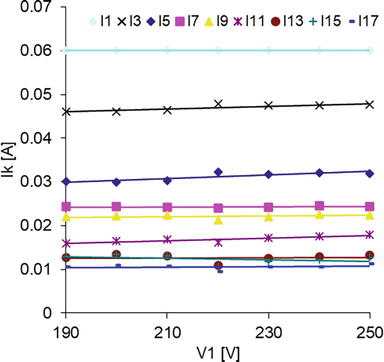
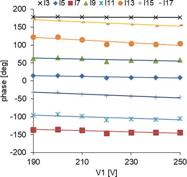
A network analyzer is a more sophisticated device which measures a set of several hundred time—samples to characterize a current waveform. A program for the computation of the modules and phases of the harmonic components delivers accurate values of these magnitudes. The results of this kind of measurement and computations are described in Ref. [10]. The FD models are given as results of linear interpolations of the measured data in the format proposed in Ref. [3]. Some results are given below for several devices (Figures 10 and 11, Tables 2–8).

Figure 10.

RMS values of the current harmonics for a CFL 10 W.

Figure 11.

Phases of the current harmonics for a CFL 10 W.

RMS [A]	PHASE [°]
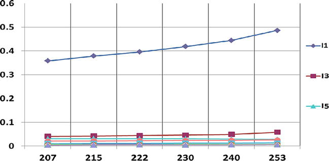
rms(I1) = −5E-18 V1 + 6E-2	ph(I1) = 0
rms(I3) = 3E-5 V1 + 4E-2	ph(I3) = −2.8E-2 Φ1 + 184
rms(I5) = 4E-5 V1 + 2.2E-2	ph(I5) = −0.11 Φ1 + 35
rms(I7) = 1E-6 V1 + 2.4E-2	ph(I7) = −0.17 Φ1-102
rms(I9) = 7E-6 V1 + 2.1E-2	ph(I9) = −0.14 Φ1 + 90
rms(I11) = 3E-5 V1 + 1E-2	ph(I11) = −0.21 Φ1-55
rms(I13) = 2E-7 V1 + 1.3E-2	ph(I13) = −0.38 Φ1 + 193
rms(I15) = −2E-5 V1 + 1.6E-2	ph(I15) = −0.27 Φ1 + 20
rms(I17) = 6E-6 V1 + 9.3E-3	ph(I17) = −0.3 Φ1 + 228

Table 2.

TFD model for a CFL 10 W.

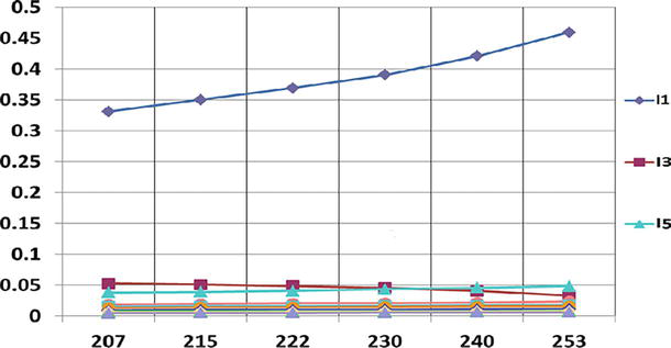
RMS [A] for LED 5 W	PHASE [°] for LED 5 W
rms(I1) = 0.2	ph(I1) = 0
rms(I3) = 2E-5 V1 + 1.3E-2	ph(I3) = −0.06 Φ1 + 186
rms(I5) = 4E-5 V1 + 4.6E-3	ph(I5) = −0.17 Φ1 + 33
rms(I7) = 3E-5 V1 + 2.7 E-3	ph(I7) = −0.39 Φ1-83
rms(I9) = 1E-5 V1 + 5.3E-3	ph(I9) = −0.49 Φ1 + 136
rms(I11) = 2E-5 V1 + 3.2E-3	ph(I11) = −0.48 Φ1-33
rms(I13) = 3E-5 V1-8.2E-4	ph(I13) = −0.64 Φ1 + 197
rms(I15) = 2E-5 V1-2.8E-4	ph(I15) = −0.95 Φ1 + 106
rms(I17) = 2E-5 V1-1.1E-3	ph(I17) = −0.98 Φ1 + 315

Table 3.

FD model for LED 5 W.

RMS [A] for LED 17 W	PHASE [°] for LED 17 W
rms(I1) = −3.9E-4 V1 + 1.6E-1	ph(I1) = 0
rms(I3) = −2.3E-4 V1 + 1.2E-1	ph(I3) = −3.9E-2 Φ1 + 185
rms(I5) = −5E-5 V1 + 6 E-2	ph(I5) = −0.17 Φ1 + 38
rms(I7) = −2E-5 V1 + 4E-2	ph(I7) = −0.44 Φ1-67
rms(I9) = −8E-5 V1 + 4.6E-2	ph(I9) = −0.54 Φ1 + 157
rms(I11) = −3E-5 V1 + 3.2E-2	ph(I11) = −0.55 Φ1-5
rms(I13) = 4E-5 V1 + 1.1E-2	ph(I13) = −0.77 Φ1 + 241
rms(I15) = 7E-6 V1 + 1.4E-2	ph(I15) = −1.11 Φ1 + 157
rms(I17) = 2E-5 V1 + 6.5E-3	ph(I17) = −1.12 Φ1+ 362

Table 4.

FD model for LED 17 W.

RMS [A] for air conditioner (heating)	Phase [°] for air conditioner (heating)
rms(I1) = −7E-3 V1 + 6.14	ph(I1) = 0
rms(I3) = −1.6E-3 V1 + 1.21	ph(I3) = −0.1 Φ1 + 142
rms(I5) = 7E-4 V1 + 0.47	ph(I5) = −0.02 Φ1-92
rms(I7) = 4E-4 V1 + 0.16	ph(I7) = 0.14 Φ1-34
rms(I9) = −8E-4 V1 + 0.32	ph(I9) = −0.21 Φ1 + 118
rms(I11) = 8E-4 V1 + 1.6E-2	ph(I11) = −0.18 Φ1-122
rms(I13) = 5E-4 V1 - 5E-2	ph(I13) = 0.88 Φ1-245
rms(I15) = −7E-4 V1 + 0.21	ph(I15) = −0.28 Φ1 + 52
rms(I17) = 5E-4 V1-4.5E-2	ph(I17) = −0.02 Φ1 + 108

Table 5.

FD model for air conditioner (heating).

RMS [A] for air conditioner (cooling)	PHASE [°] for air conditioner (cooling)
rms(I1) = −5E-3 V1 + 3.38	ph(I1) = 0
rms(I3) = −1.5E-3 V1 + 1.94	ph(I3) = −0.24 Φ1 + 192
rms(I5) = 1.8E-3 V1 + 0.32	ph(I5) = −0.29 Φ1-19
rms(I7) = −1.2E-3 V1 + 0.49	ph(I7) = 0.01 Φ1-15
rms(I9) = −5E-05 V1 + 0.31	ph(I9) = −0.66 Φ1 + 246
rms(I11) = 1.9E-3 V1-0.29	ph(I11) = −0.65 Φ1 + 17
rms(I13) = −1.4E-3 V1 + 0.39	ph(I13) = −0.86 Φ1 + 63
rms(I15) = 4E-4 V1-2E-4	ph(I15) = −1.02 Φ1 + 248
rms(I17) = −3E-4 V1 + 8.7E-2	ph(I17) = 0.88 Φ1-113

Table 6.

FD model for air conditioner (cooling).

RMS [A] for vacuum cleaner (maximum power)	Phase [°] for vacuum cleaner (maximum power)
rms(I1) = 3E-3 V1 + 3.8	ph(I1) = 0
rms(I3) = 1.6 E-2 V1-2.83	ph(I3) = 0.45 Φ1 + 83
rms(I5) = 7.8E-3 V1-1.55	ph(I5) = −0.79 Φ1 + 342
rms(I7) = 5.5E-3 V1-1.12	ph(I7) = 1.38 Φ1-243
rms(I9) = 7E-4 V1-0.11	ph(I9) = 3.62 Φ1-894
rms(I11) = 8E-4 V1-0.15	ph(I11) = −3.17 Φ1 + 783
rms(I13) = 7E-05 V1 + 4.2E-2	ph(I13) = 1.32 Φ1-103
rms(I15) = 3E-4 V1-2.3E-2	ph(I15) = −0.14 Φ1-155
rms(I17) = 1E-3 V1-0.19	ph(I17) = −1.15 Φ1 + 395

Table 7.

FD model for a VACUUM CLEANER (maximum power).

RMS [A] for refrigerator (closed door)	Phase [°] for refrigerator (closed door)
rms(I1) = 2E-3 V1 + 0.48	ph(I1) = 0
rms(I3) = −5E-5 V1 + 1.2E-1	ph(I3) = 0.32 Φ1-196
rms(I5) = −4E-4 V1 + 1.3E-1	ph(I5) = 1.41 Φ1-388
rms(I7) = −4E-5 V1 + 1.9E-2	ph(I7) = 0.85 Φ1-274
rms(I9) = 5E-5 V1-6.1E-3	ph(I9) = −4.17 Φ1+ 840
rms(I11) = −3E-6 V1 + 2.7E-3	ph(I11) = 1.27 Φ1-229
rms(I13) = 1E-5 V1-8E-4	ph(I13) = −7.32 Φ1 + 1615
rms(I15) = 1E-5 V1-1.9E-3	ph(I15) = −3.95 Φ1 + 845
rms(I17) = −2E-5 V1 + 4.7E-3	ph(I17) = 2.95 Φ1-716

Table 8.

FD model for a refrigerator.

The FD models of other nonlinear loads containing diode rectifiers are given below [10].

The appliance has an automatic power management system that tries to keep the cooling capacity constant. This effect becomes evident when considering the decreasing dependence of I₁ on V₁. A similar effect can also be observed with a 17 W LED.

The FD models for other devices or other operating conditions are described in Ref. [10], also.

The content of the paragraph “2. Current sources models with parameters determined by measurements” reproduces the research reported for the first time in Ref. [10].

4. Frequency domain models for nonlinear devices with firing angle control devices

This section discusses the frequency domain models of a nonlinear load with a firing angle controller. The conduction state of devices such as thyristors, IGBTs (insulated gate bipolar transistors), TRIACs (triodes for alternating current), and DIACs (diodes for alternating current) is controlled by command signals [11].

4.1 Input-output models depending on firing angle and input voltage: Simulations

The models developed in the above sections characterize only the input behavior of a circuit block, which is a load in a power system. Sometimes, a load in the power system is a two-port: one port being its connection with the power system and the second port being associated with output quantities of interest. The models presented in this section can be developed on the basis of datasets obtained from network analyzer measurements or simulations with dedicated software.

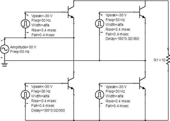
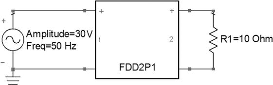
In this section, we simulate a single-phase, fully controlled four-transistor bridge rectifier driven by a sinusoidal voltage source with amplitude V = 30 V and frequency f = 50 Hz (Figure 12). The load is a 10 ohms resistive load [12]. The following procedure can also be used for any type of nonlinear firing angle control device.

Figure 12.

Single-phase fully controlled bridge rectifier.

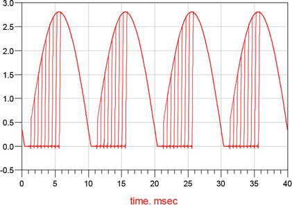
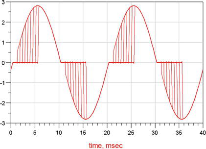
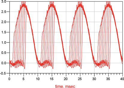
In this example, the firing angle is swept from 10 to 90 degrees with a 10-degree increment. The output port current (the load current) and input port current (the voltage source current) for all firing angles are shown in Figures 13 and 14.

Figure 13.

The output port current.

Figure 14.

The input port current.

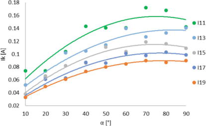
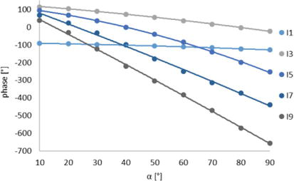
The RMS value of the first five odd harmonic components of the input current varies with the firing angle α, as shown in Figure 15, and the RMS value of the next five odd harmonic components of the input current varies with the firing angle α, as shown in Figure 16.

Figure 15.

RMS of odd current harmonics (1st-9th) vs. firing angle—Input port current.

Figure 16.

RMS of odd current harmonics (11th–19th) vs. firing angle—Input port current.

Starting from these samples, the α dependence for the most important odd input current harmonic RMS values has been computed by quadratic interpolation:

mag(I₁) = −1.63E-4·α²-2.25E-3·α + 2.78E+0.

mag(I₃) = −1.46E-4·α² + 2.39E-2·α - 8.59E-2.

mag(I₅) = −1.62E-5·α² + 3.38E-3·α + 9.87E-2.

mag(I₇) = −6.75E-5·α² + 8.22E-3·α + 1.09E-1.

mag(I₉) = −1.50E-5·α² + 2.91E-3·α + 6.37E-2.

mag(I₁₁) = −2.29E-5·α² + 3.43E-3·α + 2.95E-2.

mag(I₁₃) = −1.62E-5·α² + 2.70E-3·α + 2.50E-2.

mag(I₁₅) = −1.81E-5·α² + 2.68E-3·α + 1.54E-2.

mag(I₁₇) = −1.47E-5·α² + 2.26E-3·α + 1.47E-2.

mag(I₁₉) = −1.18E-5·α² + 1.86E-3·α + 1.64E-2.

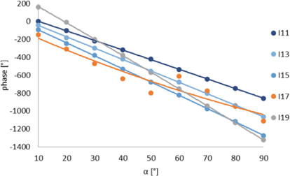
After a similar technique, the variation of the first five odd harmonic components of the phase input current with α is shown in Figure 17, and the variation of the next five odd harmonic components of the phase input current with α is shown in Figure 18.

Figure 17.

Phase of odd current harmonics (1st-9th) vs. firing angle—Input port current.

Figure 18.

Phase odd current harmonics (11th–19th) vs. firing angle—Input port current.

From these samples, the phase dependence of the most important odd harmonics of the input current on α is calculated by quadratic interpolation:

phase(I₁) = −2.35E-3·α²-2.27E-1·α - 8.96E+1.

phase(I₃) = −5.88E-3·α²-1.17E+0·α + 1.28E+2.

phase(I₅) = −2.52E-2·α²-1.86E+0·α + 1.14E+2.

phase(I₇) = −6.10E-3·α²-5.93E+0·α + 1.38E+2.

phase(I₉) = −5.44E-3·α²-8.21E+0·α + 1.25E+2.

phase(I₁₁) = −6.83E-4·α²-1.07E+1·α + 1.09E+2.

phase(I₁₃) = −1.36E-3·α²-1.26E+1·α + 8.18E+1.

phase(I₁₅) = 3.35E-2·α²-1.40E+1·α - 5.20E+1.

phase(I₁₇) = −7.93E-3·α²-1.78E+1·α + 3.45E+2.

phase(I₁₉) = −4.11E-3·α²-1.43E+1·α + 4.93E+1.

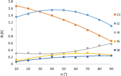
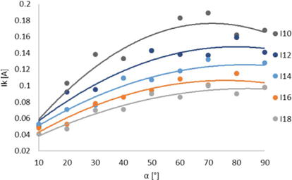
Similarly, the variation of the amplitude of the first five even harmonic components of the output current with the firing angle is shown in Figure 19, and the variation of the amplitude of the next five even harmonic components of the output current with the firing angle is shown in Figure 20.

Figure 19.

RMS of even current harmonics (DC-8th) vs. firing angle—Output port current.

Figure 20.

RMS of even current harmonics (10th–18th) vs. firing angle—Output port current.

The dependence of the most significant even output current harmonics amplitudes on the firing angle is calculated by quadratic interpolation based on the following samples:

mag(I₀) = −6.39E-5·α²-6.40E-3·α + 1.75E+0.

mag(I₂) = −2.03E-4·α² + 1.73E-2·α + 1.19E+0.

mag(I₄) = 8.11E-5·α²-4.54E-3·α + 3.55E-1.

mag(I₆) = −7.29E-5·α² + 9.56E-3·α - 8.38E-3.

mag(I₈) = −2.96E-5·α² + 5.01E-3·α + 2.43E-2.

mag(I₁₀) = −3.13E-5·α² + 4.46E-3·α + 1.69E-2.

mag(I₁₂) = −1.87E-5·α² + 2.98E-3·α + 2.88E-2.

mag(I₁₄) = −1.40E-5·α² + 2.32E-3·α + 2.93E-2.

mag(I₁₆) = −1.46E-5·α² + 2.21E-3·α + 2.22E-2.

mag(I₁₈) = −1.06E-5·α² + 1.78E-3·α + 2.16E-2.

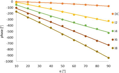
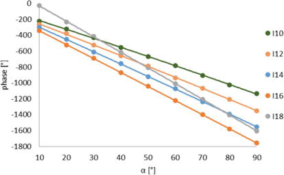
The variation of the phase of the first five even harmonic components of the input current with the firing angle is shown in Figure 21, and the variation of the phase of the next five even harmonic components of the input current with the firing angle is shown in Figure 22.

Figure 21.

Phase of even current harmonics (2nd-8th) vs. firing angle—Output port current.

Figure 22.

Phase of even current harmonics (10th–18th) vs. firing angle—Output port current.

The phase dependence of the most important even harmonic output current components on α is calculated by quadratic interpolation starting from these data:

phase(I₂) = −5.42E-3·α²-4.03E-1·α + 2.64E+0.

phase(I₄) = −1.42E-3·α²-3.89E+0·α + 2.99E+1.

phase(I₆) = 7.53E-3·α²-6.49E+0·α + 8.47E+0.

phase(I₈) = −9.28E-4·α²-7.60E+0·α - 3.69E+1.

phase(I₁₀) = −8.80E-3·α²-8.75E+0·α - 8.11E+1.

phase(I₁₂) = −7.12E-3·α²-1.09E+1·α - 1.05E+2.

phase(I₁₄) = −7.50E-3·α²-1.29E+1·α - 1.27E+2.

phase(I₁₆) = −4.53E-3·α²-1.52E+1·α - 1.46E+2.

phase(I₁₈) = −3.57E-3·α²-1.73E+1·α - 1.70E+2.

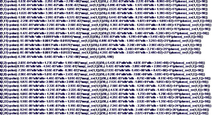
4.2 New input-output FD model implementation

Ideally, the grid provides a constant RMS voltage, such as 230 V. The voltage is considered a constant RMS value, even if it fluctuates within a small range. Therefore, we can say that, under normal conditions, circuits operate at constant magnitude values at and around the supply voltage, and the next model of the current source type is proposed. This model uses a current source controlled by the input voltage. Each current harmonic is described by its magnitude and phase. The control parameters are the amplitude and phase of the fundamental component of the input voltage and the firing angle. This is the first improvement of the model presented in this section. The second improvement of the same model is its implementation in ADS using a Frequency Domain Defined 2-Port component (FDD2P), and its validation by simulations leading to the same results as those obtained by the simulation of the circuit in Figure 23.

Figure 23.

Nonlinear controlled source model of circuit in Figure 12.

The equations obtained in the previous section and the magnitude and phase dependencies are implemented in the ADS software, as shown in Figures 24–26.

Figure 24.

Model implementation in ADS.

Figure 25.

The output port current—Simulated.

Figure 26.

The input port current—Simulated.

One major advantage of this type of FD model is the reduction of the simulation time. In Table 9, the CPU times for the simulations of the circuit in Figure 12 using the TD model and using the FD model for the HB analysis are given.

Model	CPU time [s]
TD	8.80
FD	2.37

Table 9.

Simulation results.

An input-output FD model for a full-controlled bridge rectifier with four transistors has been presented in this section. The model consists of two sets of equations and can be extended to circuits with multiple ports. The models presented in this section can be obtained by using a network analyzer to make magnitude and phase measurements of all harmonic components of interest, or from datasets obtained using circuit simulation software that provides odd and even current harmonics. This model is characterized by a quadratic dependence of the amplitudes and phases of the current harmonics on the firing angle at the same input voltage. FD models reduce simulation time compared to classic HB analysis using TD models. To further improve the accuracy of the model, the number of considered harmonics can be increased, and the interpolation approximation function can be improved. However, the number of harmonics considered must be chosen carefully, as it increases simulation time without appreciably improving results. This type of FD model can also be used for larger circuits and networks. In this case, it is foreseeable that the simulation time will be significantly reduced compared to the classical model. Another important advantage is after the computation of the model parameters, a lot of new simulations can be performed in a considerably shorter time than a customary analysis.

4.3 Models depending on firing angle and input voltage: Measurements

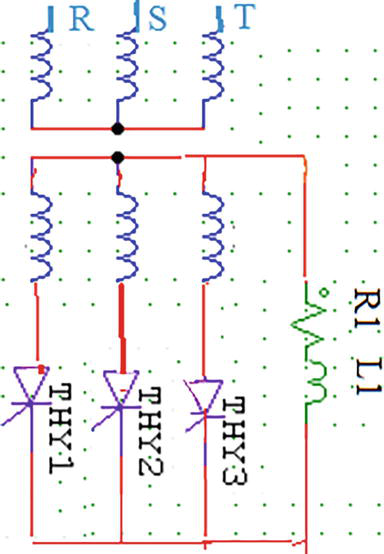
Some measurements on one-phase and three-phase thyristor rectifiers (Figures 27 and 28), which may lead to their frequency domain models, are reported in this section together with an FD model of a one-phase rectifier with two thyristors.

Figure 27.

One-phase rectifier.

Figure 28.

Three-phase rectifier.

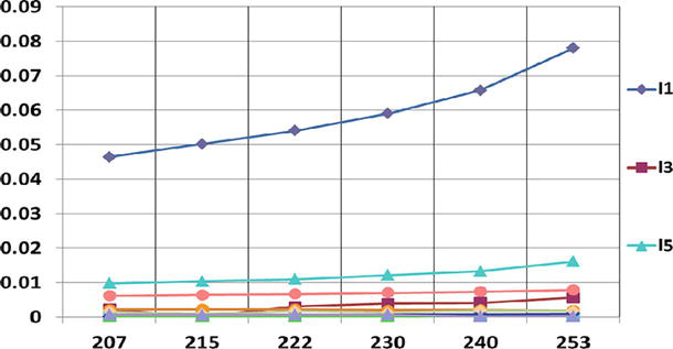
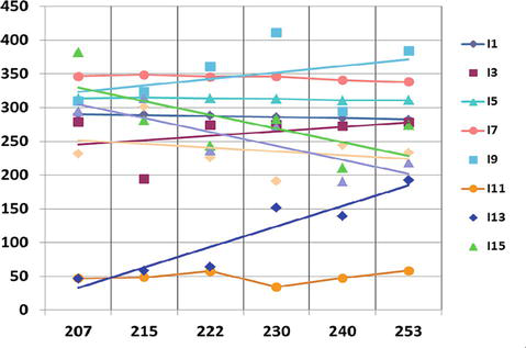
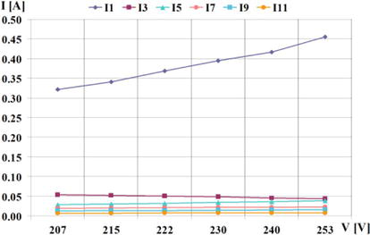
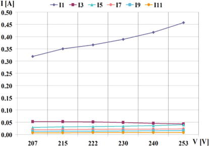
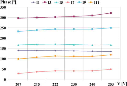
The current harmonics amplitudes and phases, depending on the fundamental component of the voltage, are measured for various values of the firing angle (Figures 29–38) in the case of the one-phase rectifier.

Figure 29.

RMS values for I1—I19 for α = 21°.

Figure 30.

PHASE values for I1—I19 α = 21°.

Figure 31.

RMS values for I1—I19 for α = 50°.

Figure 32.

PHASE values for I1—I19 for α = 50°.

Figure 33.

RMS values for I1—I19 for α = 70°.

Figure 34.

PHASE values for I1—I19 for α = 70°.

Figure 35.

RMS values for I1—I19 for α = 90°.

Figure 36.

PHASE values for I1—I19 for α = 90°.

Figure 37.

RMS values for I1—I19 for α = 150°.

Figure 38.

PHASE values for I1—I19 for α = 150°.

The following measurement results are obtained for one phase of the three-phase rectifier in Figures 28, 39–48.

Figure 39.

RMS values for α = 21°.

Figure 40.

PHASE values for α = 21°.

Figure 41.

RMS values for α = 50°.

Figure 42.

PHASE values for α = 50°.

Figure 43.

RMS values for α = 70°.

Figure 44.

PHASE values for α = 70°.

Figure 45.

RMS values for α = 90°.

Figure 46.

PHASE values for α = 90°.

Figure 47.

RMS values for α = 121°.

Figure 48.

PHASE values for α = 121°.

Similar results have been obtained for the other two phases of the rectifier.

4.4 Frequency domain model of a one-phase two thyristors rectifier

From the measurement results, it follows that a useful model of a one-phase thyristor rectifier must compute the dependencies of the RMS and phase values of each current harmonic component on V₁ and phase(V₁), starting from the measured dependencies on V₁ for a set of firing angles. The simplest dependence on V₁ and phase(V₁) is a polynomial of two variables, which can be easily implemented in ADS software.

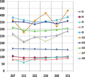
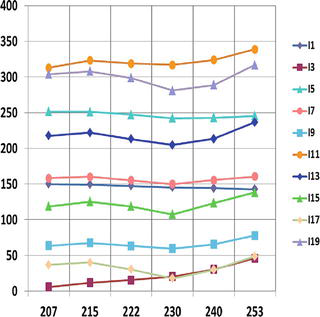
In order to verify the validity of our approach, we ignore the measured values for α₃ = 70⁰ and try to compute them using two interpolation polynomials. The current amplitudes and phases of the current harmonics have been measured for the following values of V₁ and α (Tables 10 and 11).

${\mathrm{U}}_1$ [V]	${\mathrm{U}}_2$ [V]	${\mathrm{U}}_3$ [V]	${\mathrm{U}}_4$ [V]	${\mathrm{U}}_5$ [V]	${\mathrm{U}}_6$ [V]
207	215	222	230	240	253

Table 10.

V₁ values.

α1 [°]	α2 [°]	α3 [°]	α4 [°]	α5 [°]	α6 [°]
21	50	70	90	126	150

Table 11.

Firing angles values.

To verify the validity of our approach, we ignore the measured values for α₃ = 70⁰ and compute them using several interpolation methods:

• the poly45 function, which is a polynomial implemented in MATLAB and is based on the measured results for four values of α and five values of V₁,

• other interpolation polynomials, based on five values for α and six values of V₁.

Finally, these results are compared with those given by a genetic algorithm based on the current samples measured by the network analyzer [13].

Interpolation algorithm: Giving the measured current samples $i_j=i\left(t_j\right),\mathrm{j}=\overline{1,S}$, the RMS values $I_{2k-1}$ and initial phases ${\phi }_{2k-1}$ for the fundamental component and the odd harmonics up to the 11th order $\left(k=\overline{1,6}\right)$ are calculated so that the sum of the above components represents the best approximation of the measured current waveform:

$$i\left(t\right)=\sum _{k=1}^6\sqrt{2}{I}_{2k-1}\mathit{sin}\left(\left(2k-1\right)\mathit{\omega t}+{\phi }_{2k-1}\right)$$E1

To this end, the following error function is defined:

$$\mathit{ERR}\left(I_1,{\phi }_1,I_3,{\phi }_3,\dots ,I_{11},{\phi }_{11}\right)=\sum _{i=1}^S{\left[i_j-i\left(t_j\right)\right]}^2$$E2

Introducing (1) in (2) it follows:

$$\mathit{ERR}\left(I_1,{\phi }_1,I_3,{\phi }_3,\dots ,I_{11},{\phi }_{11}\right)=\sum _{j=1}^S{\left[i_j-\sum _{k=1}^6\sqrt{2}{I}_{2k-1}\mathit{sin}\left(\left(2k-1\right)\omega t_j+{\phi }_{2k-1}\right)\right]}^2$$E3

This error function has 12 variables, so a solution vector x with 12 components is defined to minimize the value of the above function using MATLAB. The corresponding relationship between the solution vector and each component of x is:

$$A_{2k-1}\to x_{2k-1},{\phi }_{2k-1}\to x_{2k},k=\overline{1,6}$$E4

Employing (4) in (3), we obtain:

$$\mathit{ERR}\left(x_1,x_2,\dots ,x_{11},x_{12}\right)=\sum _{j=1}^S{\left[i_j-\sum _{k=1}^6\sqrt{2}{x}_{2k-1}\mathit{sin}\left(\left(2k-1\right)\omega t_j+x_{2k}\right)\right]}^2$$E5

The error function in (5) was generated with MAPLE and converted into the MATLAB code. This error function value can be minimized using the MATLAB function ga from the Global Optimization Toolbox. This minimization method uses a genetic algorithm to find the RMS value and phase of the odd harmonic components of order 1–11. To do this, the ga function uses the following options: “HybridFcn”, @fminunc, “Generations”, 1200, “TolFun”, 1e-15.

In this way, the algorithm calculates the RMS and initial phase values of the six odd harmonic current components for a set of $M\times N$ points defined by the values of the fundamental voltage components $U_m,m=\overline{1,M}$ and the values of firing angle ${\alpha }_n,n=\overline{1,N}$.

To calculate the same RMS and initial phase values of the six odd harmonic components at the new point, the polynomial interpolation described below is used. That is, in order to calculate the RMS value I_k and the initial phase φ_k of the k^th current harmonic, two $\left(M-1\right)\times \left(N-1\right)$-order interpolation polynomials are built. Here are the two variable polynomials in U and $\alpha$:

$$\begin{array}{rcl}{P}_{I_k}\left(U,\alpha \right)& =& \sum _{i=1}^M\left(U^{i-1}\sum _{j=1}^N{A}_{j+\left(i-1\right)·N}{\alpha }^{j-1}\right)\\ & =& A_1+A_2\alpha +\dots A_N{\alpha }^{N-1}+A_{N+1}U+\dots +A_{2N}U{\alpha }^{N-1}+\dots \\ & & +A_{1+\left(M-1\right)·N}{U}^{M-1}+\dots +A_{M·N}{U}^{M-1}{\alpha }^{N-1}\end{array}$$E6

$$\begin{array}{rcl}{P}_{{\phi }_k}\left(U,\alpha \right)& =& \sum _{i=1}^M\left(U^{i-1}\sum _{j=1}^N{B}_{j+\left(i-1\right)·N}{\alpha }^{j-1}\right)\\ & =& B_1+B_2\alpha +\dots B_N{\alpha }^{N-1}+B_{N+1}U+\dots +B_{2N}U{\alpha }^{N-1}+\dots \\ & & +B_{1+\left(M-1\right)·N}{U}^{M-1}+\dots +B_{M·N}{U}^{M-1}{\alpha }^{N-1}\end{array}$$E7

These polynomials are constructed in such a way that their computation yields the RMS value of I_k and the initial phase of I_k, which correspond to the fundamental voltage component $U_m$ and firing angle ${\alpha }_n$:

$$P_{I_k}\left(U_m,{\alpha }_n\right)=\sum _{i=1}^M\left(U_m^{i-1}\sum _{j=1}^N{A}_{j+\left(i-1\right)·N}{\alpha }_n^{j-1}\right)=I_k\left(U_m,{\alpha }_n\right)$$E8

$$P_{{\phi }_k}\left(U_m,{\alpha }_n\right)=\sum _{i=1}^M\left(U_m^{i-1}\sum _{j=1}^N{B}_{j+\left(i-1\right)·N}{\alpha }_n^{j-1}\right)={\phi }_k\left(U_m,{\alpha }_n\right)$$E9

The computation of the coefficients $A_{j+\left(i-1\right)·N}$, respectively $B_{j+\left(i-1\right)·N}$, $i=\overline{1,M}$, $j=\overline{1,N}$ is done by solving the following equation systems:

$$\begin{array}{l}{A}_1+A_2{\alpha }_n+\dots +A_{j+\left(i-1\right)·N}{U}_m^{i-1}{\alpha }_n^{j-1}+\dots +A_{M·N}{U}_m^{M-1}{\alpha }_n^{N-1}=I_k\left(U_m,{\alpha }_n\right),\\ m=\overline{1,M},n=\overline{1,N},\\ \left(i=\overline{1,M},j=\overline{1,N}\right)\end{array}$$E10

$$\begin{array}{l}{B}_1+B_2{\alpha }_n+\dots +B_{j+\left(i-1\right)·N}{U}_m^{i-1}{\alpha }_n^{j-1}+\dots +B_{M·N}{U}_m^{M-1}{\alpha }_n^{N-1}={\phi }_k\left(U_m,{\alpha }_n\right),\\ m=\overline{1,M},n=\overline{1,N},\\ \left(i=\overline{1,M},j=\overline{1,N}\right)\end{array}$$E11

Knowing the values of the coefficients $A_{j+\left(i-1\right)·N}$, and $B_{j+\left(i-1\right)·N}$, for $i=\overline{1,M}$, and $j=\overline{1,N}$, the algorithm computes the RMS value and the initial phase of the k^th current harmonic in a point corresponding to the fundamental voltage RMS value U′,$U_1\le U^{\prime }\le U_M$, and to the firing angle α’, ${\alpha }_1\le {\alpha }^{\prime }\le {\alpha }_N$, as:

$$I_k\left(U^{\prime },{\alpha }^{\prime }\right)=P_{I_k}\left(U^{\prime },{\alpha }^{\prime }\right)=\sum _{i=1}^M\sum _{j=1}^N{A}_{j+\left(i-1\right)·N}{\alpha }^{\prime j-1}{U}^{\prime i-1}$$E12

$${\phi }_k\left(U^{\prime },{\alpha }^{\prime }\right)=P_{{\phi }_k}\left(U^{\prime },{\alpha }^{\prime }\right)=\sum _{i=1}^M\sum _{j=1}^N{B}_{j+\left(i-1\right)·N}{\alpha }^{\prime j-1}{U}^{\prime i-1}$$E13

In order to compare the results, the magnitudes in (12) and (13) are computed with the function fit from the Curve Fitting Toolbox of MATLAB. The parameter fitType is “poly45”, and in this case, the polynomial has the order 4×5, its variables being α_n U_m. Obviously, the FD models are the curves I_k(U_m, α_n) α_n = ct and φ_k(U_m, α_n) α_n = ct obtained from (8) and (9) or from (12) and (13). These are polynomials in U_m and may be considered as a generalization of the linear models in (1). This kind of model can be easily implemented in ADS.

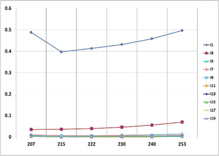
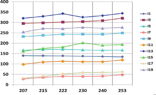
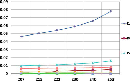
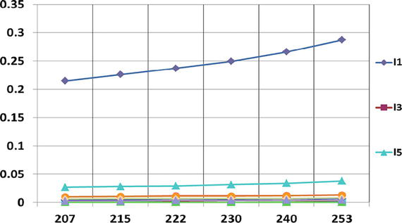
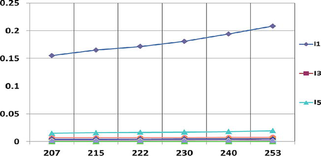
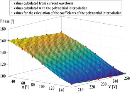
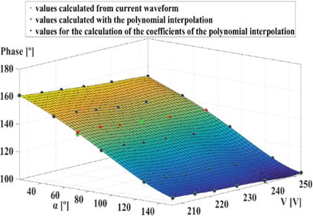
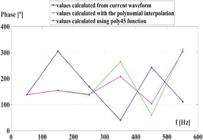
Results: The performance of the model obtained using the Poly45 function (MATLAB) and the polynomial interpolation described in the previous section is shown below. The RMS values of the dependence of the fundamental current components on U and α are represented by the red dots in Figure 49.

Figure 49.

First harmonic RMS value vs. U and α (poly45).

This dependence is compared to that of the genetic algorithm in Ref. [14], based on the measured time samples (green dots). If there is no measurement data for α = 70⁰, the measurement points correspond to 6 values of U and 5 values of α, so the poly45 function chooses the best 20 points to create the interpolating polynomial (blue points).

The error measure for this interpolation method is the distance between each pair of green and red points in Figure 49.

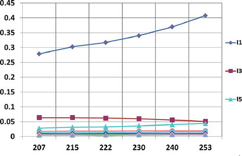
Figure 50 shows a similar interpolation error measurement for the initial phase of the fundamental component of the current computed using poly45 (MATLAB).

Figure 50.

First harmonic initial phase value vs. U and α (poly45).

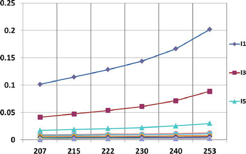
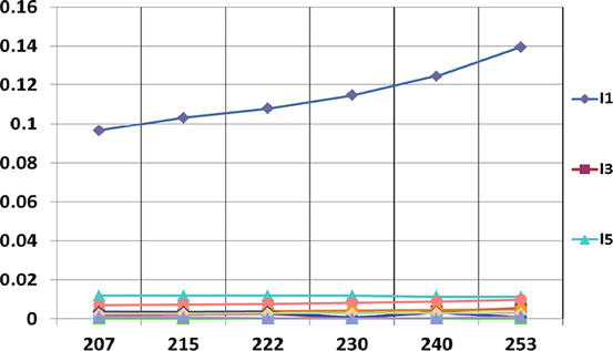
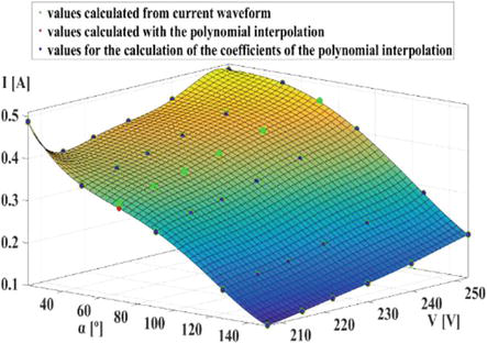
The error of the proposed interpolation method can be estimated by analyzing Figures 51 and 52. A simple inspection of the distance between each pair of green and red points shows that the proposed interpolation method gives better results than the poly45 function (MATLAB).

Figure 51.

First harmonic RMS value vs. U and α (proposed interpolation).

Figure 52.

First harmonic initial phase value vs. U and α (proposed interpolation).

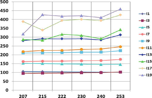
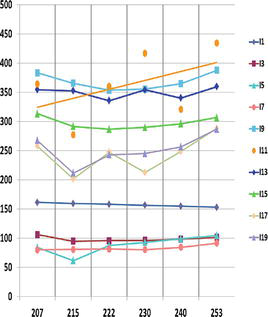
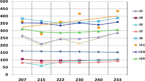
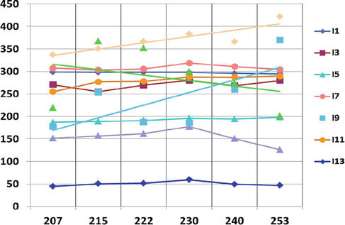
Below, the RMS values and the initial phase values dependences on U of all odd current harmonics obtained by the two interpolation algorithms with α = 70⁰ are compared with the same dependences given by the genetic algorithm in Ref. [14], which are based on the measured time samples and is regarded as the minimum error data (Figures 53–58).

Figure 53.

RMS values vs. U for α = 70⁰ obtained with the genetic algorithm [14].

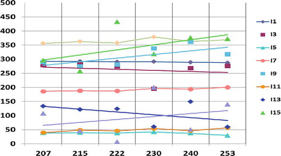
Figure 54.

RMS values vs. U for α = 70⁰ obtained with poly45 (MATLAB).

Figure 55.

RMS values vs. U for α = 70⁰ obtained with the proposed interpolation.

Figure 56.

Phases vs. U for α = 70⁰ obtained with the genetic algoritm [13].

Figure 57.

Phases vs. U for α = 70⁰ obtained with poly45 (MATLAB).

Figure 58.

Phases vs. U for α = 70⁰ obtained with the proposed interpolation.

A simple inspection of Figures 49–52 shows that the results obtained using the poly45 function (MATLAB) and the proposed interpolation algorithm are very close to those of the genetic algorithm based on measurement time samples in Ref. [14]. From Figures 56–58, it can be seen that the initial phase obtained using the poly45 function (MATLAB) and the proposed interpolation has a significant error compared to the initial phase obtained by the genetic algorithm in Ref. [14], unlike the RMS values.

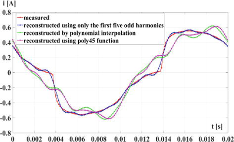
Another possibility for different methods of error estimation is waveform reconstruction. Figure 59 shows the following current waveforms: measured (red line), reconstructed using the algorithm in Ref. [14] (blue line), reconstructed using Poly45 interpolation (pink line), and reconstructed using the proposed polynomial interpolation (green line).

Figure 59.

Measured and reconstructed current waveforms for α = 70⁰ and U = 230 V.

It is obvious that the waveform obtained using the genetic algorithm in Ref. [14] is closest to the measured waveform.

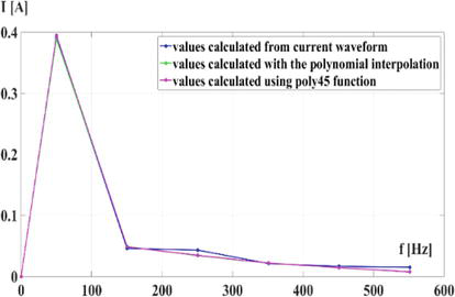
To measure such errors, Figure 60 shows the spectrum of RMS values at α = 70⁰ and U = 230 V obtained using the poly45 interpolation algorithm (red line) and the proposed interpolation algorithm (green line) in comparison with the spectrum (blue line) corresponding to the RMS value calculated by the algorithm in Ref. [14]. At first glance, all results are very close.

Figure 60.

RMS current harmonics spectrum.

The phase spectrum at α = 70⁰ and U = 230 V calculated using the same algorithm is shown in Figure 61. In this case, some important errors can be noted.

Figure 61.

Initial phase current harmonics spectrum.

4.5 Comparison between interpolation algorithms

Since the losses in the transmission line are proportional to I² (I – RMS value of the current), this value can be used as a failure criterion for the algorithm to calculate the current harmonics. The RMS current value can be calculated using the well-known formula:

$$I=\sqrt{{\sum }_{k=1}^6{I}_{2k-1}^2}=\sqrt{I_1^2+I_3^2+I_5^2+I_7^2+I_9^2+I_{11}^2}$$E14

The values of I₁ and I obtained using various algorithms using (14) are given in Table 12.

	Genetic algorithm [8]	Proposed interpolation algorithm	“poly45” (MATLAB)
$I_1$ [mA]	390.471	389.063	394.656
$I$ [mA]	396.683	394.537	400.050

Table 12.

RMS values computed from I_k.

The RMS value of I can be calculated using time samples of the current waveform (Table 13).

	Measured	Genetic algorithm [8]	Proposed interpolation algorithm	Interpolation using “poly45”
$I$[mA]	396.925	396.395	394.676	400.285

Table 13.

RMS values computed from time samples.

$$i_j=i\left(t_j\right),j=\overline{1,S}$$E15

$$\mathrm{as}:I=\sqrt{\frac{1}{S}{\sum }_{j=1}^S{i}_j^2}$$E16

The maximum relative error between the RMS values of I calculated with different algorithms is 1.5%, so these results can be considered similar from a practical point of view.

Unlike diode rectifiers, whose behavior is determined only by the parameters V₁ and phase(V₁), the behavior of a rectifier with two thyristors is determined by an additional parameter: the firing angle α. For certain values of α (in the case of the two thyristors rectifier for α = 21⁰), the dependence of I₁ on U is nonlinear, so the linear small-signal model used in Refs. [8, 9, 10] is not valid. This is because the building of the FD model requires a relatively complex interpolation algorithm, as described in this section. The model consists of higher-order polynomials representing the surface, as shown in Figures 49–52, cross sections α = ct. Further research will be devoted to the FD models of the IGBT circuits.

Since the FD model of the diode rectifier achieves an order of magnitude reduction in CPU time compared to the HB analysis using the TD diode model [8], it is expected that the FD model of the firing angle control devices will lead to a similar reduction in simulation time.

The content of paragraph “3. Frequency domain models for nonlinear devices with firing angle control devices” reproduces the research reported for the first time in Refs. [12, 15].

5. FD and TD models efficiency

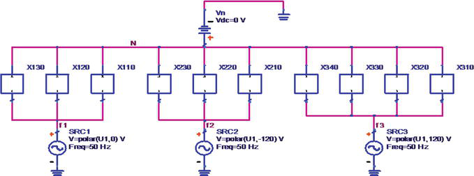
A three-phase test circuit with 10 identical loads (Figure 62), each consisting in 10 rectifiers, connected to a three-phase sinusoidal source with f = 50 Hz and amplitude V = 230 V has been used for a comparison of the simulation times obtained with HB method of ADS using the FD models proposed in Ref. [8], HB method of ADS using the usual TD models, and the following analyses implemented in CADENCE using TD models: TRAN, PSS TRAN, and PSS-HB [16].

Figure 62.

Three-phase test circuit.

Each rectifier is connected to the 400 m line by a 6mm² cable of 30 m with R_phase = 4.767 Ω/Km and X_phase = 0.101 Ω/Km. Each sinusoidal source is connected to the load by a line of 400 m with R_line = 0.045 Ω/Km and X_line = 0.074 Ω/Km. Each group of loads contains five one-diode rectifiers and five two-diode rectifiers, as those in Figures 1 and 4. This home appliance is a non-equilibrated circuit containing 150 capacitors, 150 diodes, 100 inductors, and 200 resistors (Figure 62).

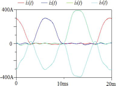
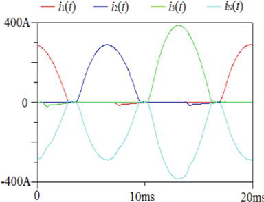
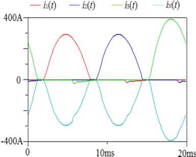
The phase currents i₁(t), i₂(t), i₃(t) are pointed out in Figures 63 and 64, and i_N(t) is considered through V_n.

Figure 63.

Currents with HB (ADS) FD models [16].

Figure 64.

Currents with HB (ADS) FD models [16].

The models used to obtain the results in Figures 63–65 are based on linear dependence outlined in Section 1. To ensure the convergence of all analyses, we added the conductance Gmin = 1e-6 Ω⁻¹ in parallel with all P-N junctions. The CPU times for all analyses are given in Table 14 [16].

Figure 65.

Currents with PSS-HB (Cadence) TD models [16].

Analysis	CPU time [s]	Peak memory used [Mbytes]
HB ADS – FD MODELS	1.36	not available
HB ADS – TD MODELS	550.34	not available
Tran ADS – TD MODELS	10.76	not available
PSS-HB Cadence – TD MODELS	215	505
PSS tran Cadence – TD MODELS	5.39	241
Tran Cadence – TD MODELS	6.88	59.6

Table 14.

Simulation results.

From Table 14 it is obvious that the HB ADS analysis using the proposed models is the most efficient. Using FD models, the results corresponding to the original circuit (Gmin = 0) can be obtained in the same CPU time as those in Table 14. To obtain the same results, a certain number of iterations using decreasing values for Gmin must be performed employing Cadence analyses [17]. This certifies that, at least for this example, the HB analysis with ADS using our proposed models is the most efficient. Other examples must be analyzed to prove if this statement is generally valid.

The content of paragraph “4. FD and TD models efficiency” reproduces the research reported for the first time in Ref. [16].

References

1.IEEE recommended practices and requirements for harmonic control in electrical power systems. In: IEEE Std 519-1992. 9 April 1993. pp. 1-112. DOI: 10.1109/IEEESTD.1993.114370. Available from: https://ieeexplore.ieee.org/
2.Pandi VR, Zeineldin HH, Xiao W. Determining optimal location and size of distributed generation resources considering harmonic and protection coordination limits. IEEE Transactions on Power Systems. 2013;28(2):1245-1254
3.Hammad AE, Kamwa I, Viarouge P, Le-Huy H, Dickinson EJ, Medina A, et al. Modeling and simulation of the propagation of harmonics in electric power networks. I: Concepts, models, and simulation techniques. IEEE Transactions on Power Delivery. 1996;11:452-465
4.Kundert KS, Sangiovanni-Vincentelli A. Simulation of nonlinear circuits in the frequency domain. IEEE Transactions on Computer-Aided Design. 1986;CAD-5(4):521-535
5.Medina A, Segundo-Ramirez J, Ribeiro P, Xu W, Lian KL, Chang GW, et al. Harmonic analysis in frequency and time domain. IEEE Transactions on Power Delivery. 2013;28(3):1813-1821
6.Nassif A. Modeling, measurement and mitigation of power system harmonics [PhD thesis] in electrical and computer engineering, University of Alberta, Edmonton, Canada. 2009
7.Yong J, Chen L, Nassif A, Xu W. A frequency-domain harmonic model for compact fluorescent lamps. IEEE Transactions on Power Delivery. 2010;25(2):1182-1189
8.Constantinescu F, Gheorghe AG, Marin ME, Taus O. Harmonic balance analysis of home appliances power networks. In: 2017 14th International Conference on Engineering of Modern Electric Systems (EMES). Oradea, Romania: IEEE; 1-2 June 2017. pp. 256-260
9.Gheorghe AG, Constantinescu F, Marin ME, Ștefănescu V, Vătășelu G. Frequency domain models for nonlinear home appliance devices. In: 2018 International Symposium on Fundamentals of Electrical Engineering (ISFEE). Bucharest, Romania: IEEE; 1-2 November 2018. pp. 1-4
10.Constantinescu F, Gheorghe AG, Marin ME, Vătășelu G, Ștefănescu V, Bodescu D. New models for frequency domain simulation of home appliances networks. In: 11-th International Symposium on Advanced Topics in Electrical Engineering. Bucharest, Romania: IEEE; 28-30 March 2019. pp. 1-5
11.Technical University “Gheorghe Asachi”, Iaşi, Romania, Faculty of Electrical Engineering and Power Engineering, Power Electronics Laboratory (in Romanian). Available from: http://www.euedia.tuiasi.ro/lab_ep/ep_files
12.Gheorghe AG, Marin ME, Dragusin MD. New frequency domain models for multiple port devices with variable firing angle. In: 2021 25th International Conference on Circuits, Systems, Communications and Computers (CSCC), Crete Island, Greece. Vol. 2021. IEEE; 2021. pp. 51-55
13.Constantinescu F, Rață M, Enache FR, Vătășelu G, Ștefănescu V, Milici D, et al. Frequency domain models for nonlinear loads with firing angle control devices part I – Measurements. In: 2019 15th International Conference on Engineering of Modern Electric Systems (ICEMES). Oradea, Romania: IEEE; 13-14 June 2019. pp. 241-246
14.Enache A, Petrescu T, Enache FR, Popescu FG. Spectrum computation for periodic analog signals using genetic algorithms. In: ICATE 2014 - International Conference on Applied and Theoretical Electricity. Craiova, Romania: IEEE; 23-25 October 2014. pp. 1-6
15.Enache FR, Constantinescu F, Rață M, Vătășelu G, Ștefănescu V, Milici D, et al. Frequency domain models for nonlinear loads with firing angle control devices, part II – Modeling. In: 6-th International Symposium on Electrical and Electronics Engineering. Galati, Romania: IEEE; 18-20 October 2019. pp. 1-6
16.Gheorghe AG, Constantinescu F, Marin ME. Time domain and frequency domain models for analysis of nonlinear power networks of home appliances. In: International Symposium on Signals, Circuits and Systems 2021. Iasi, Romania: IEEE; 15-16 July 2021. pp. 1-4
17.Lin S, Kuh ES, Marek-Sadowska M. Stepwise equivalent conductance circuit simulation technique. IEEE Transactions on Computer-Aided Design of Integrated Circuits and Systems. 1993;12(5):672-683
Written By
Florin Constantinescu, Alexandru Gabriel Gheorghe, Mihai Eugen Marin and Florin Roman Enache
Submitted: 06 June 2023Reviewed: 22 July 2023Published: 26 November 2023