Application of Simulation Modeling to Assess the Operation of Urban Toll Plazas

Abstract

This chapter deals with the simulation of traffic flow through toll plazas (hereinafter referred to as TPs) on an intraurban toll road. Toll plazas (TPs) and their functioning parameters are the sources of traffic congestion risk on toll roads. Three types of TPs are considered: at the exit from the toll road; on the main course of the road; at the exit from the road before the regulated intersection. As a transport micro-simulation methodology, discrete-event simulation of TPs using AnyLogic software is used. Each TP simulation model takes into account the specifics of traffic and user behavior. At the end of the chapter, conclusions are offered on the main factors influencing traffic congestion for each of the TPs. Based on the data obtained from the simulations, recommendations were made to improve the performance of the TP and the traffic light facility, reducing the risks of congestion on the research objects.

1. Introduction

Over the past two decades, toll roads have played a special role for countries with developing transport infrastructures, including those that are part of domestic and international transport corridors. Despite the widespread adoption of barrier-free toll system technologies, such as multilane free-flow, barrier-type toll roads, where fare collection is done with a stop-over at a TP, are prevalent in a number of countries.

One type of toll road is the intraurban toll road, which connects different parts of a city as well as suburban areas. Unlike high-speed toll roads, they are characterized by high volume of traffic, high volume of labor and recreational correspondence, cramped urban infrastructure of alignment, its transport interchanges, and TPs. Intraurban toll roads are designed to unload the street and road network of the city, accelerate movement between districts and increase the mobility of the urban population using individual cars.

Taking into account territorial restrictions on placement of engineering infrastructure, the task of ensuring maximum capacity of the implemented toll collection system (hereinafter referred to as TCS) with a minimum number of toll lanes and dimensions of the TPs zone is entrusted to the TPs of intraurban toll roads. The TCS must be configured in such a way as to ensure the best possible match with traffic flow, distribute the load on the toll lanes evenly during peak hours, and minimize downtime during the day.

These increased requirements for the configuration of the TP allow for the reduction of congestion risks on the road itself and at its connection points to the street and road network. Congestion on a toll road has a negative impact on a combination of traffic, economic, social, and environmental parameters.

Tasks of maintaining, controlling, and managing traffic flow on a toll road are usually entrusted to the operating organization operator, which manages traffic on a toll road with the help of traffic management system and is designed to ensure the efficiency of using all sections of the toll road and maintaining a high quality of user services provided. Toll roads have a capacity limit. The ability to predict anticipated changes in traffic, risks of traffic congestion, and reduction in the quality of user service is a priority and relevant to the road operator.

Various mathematical and instrumental methods can be used to assess the efficiency of the TCS functioning at the TP, one of which is simulation modeling. Simulation modeling is a highly effective and relatively inexpensive tool for assessing traffic flows, and the quality of functioning of road elements under conditions of predictable road traffic not only in road operation but also in road design.

The Western High-Speed Diameter (hereinafter referred to as WHSD), located in St. Petersburg, Russia, is considered as an example of an intraurban toll road. This project is an excellent example of the simulation method because of the variety of technical solutions that allow different system configurations to be considered. The TCS of this road can be classified as a mixed type, as its sections have features of both open and closed types of TCS, and the TPs combine different types of toll lanes, allowing for both stop and nonstop tolling.

The variety of TCS configurations allows the road operator to control the TP by adapting it to varying traffic flow parameters, the main ones being its intensity, traffic composition, and the proportion of toll collection methods used.

Thus, the need for effective management of TCS configurations at TPs, as well as the use of reliable and flexible performance evaluation tools for system configurations that can be used by the operator to improve the quality of management decision-making, is a relevant issue.

This chapter shows the results of the development and application of a simulation method to evaluate the performance of different types of intraurban TPs:

1. Toll road exit TP;

2. TP on the main course of a toll road;

3. TP at the exit from the toll road before the controlled intersection.

The conducted research allowed us to consider and evaluate the quality of operation of TPs with various configurations of TCS under different traffic flow parameters as well as to assess the risks of traffic congestion on them.

Based on the results of the study, the toll road operator can assess the current and predicted congestion of the TP, as well as plan measures to optimize and upgrade the TCS in advance.

2. Literature review

The methodology of studying TP as a queuing system and applying discrete-time modeling to it was applied by Punitha [1]. In Aksoy et al. [2], using the Fatih Sultan Mehmet Bridge toll simulation model, a number of experiments were conducted using the Vissim software to vary the TP intensity at different numbers of open toll lanes, thereby improving the quality of service. An effective methodology for evaluating the TP operation using the Generic Toll Plaza Simulation (GENTOPS) simulation model has been proposed by Aycin [3]. Similar optimization problems for the operation of toll lanes using simulation methods have been solved by Izuhara et al. [4] and Levinson & Chang [5]. An assessment of the effectiveness of TP modernizations has been investigated by Yosritzal et al. [6]. In this study, it was pointed out that the most feasible capacity increase at TP might be to upgrade the TCS system by switching to Electronic toll collection (hereinafter referred to as ETC) and multilane free-flow rather than increasing the number of existing manual toll lanes.

The use of simulation modeling is common for traffic forecasting problems at TPs. Prediction of average queue length at TP using Long Short-Term Memory model and particle swarm optimization algorithm is used by Peng et al. [7]. Munawar & Andriyanto [8] demonstrated the application of simulation modeling to solve queue waiting time prediction problems using the example of Cililitan Toll Plaza, Jakarta. Simulation modeling has been used to estimate the system delay of vehicles in manual toll lanes and ETC lanes under mixed traffic conditions in Chintaman et al. [9, 10]. However, the results of a study by Yogeshwar et al. [11] show that the level of service during toll collection includes not only the service time at the toll lanes but also many additional factors.

The introduction and application of contactless payment-type transponders at TPs, which significantly increase the toll collection rate, is actively discussed by the scientific community. The effectiveness of this method of tolling has been noted by Huang et al., Qian et al., Hewage et al., Tanino et al., Zhu et al., Ito et al., Roth, Lai et al., Lee, Tseng & Wang, Vats, Vats, Vaish & Kumar, Abuzwidah & Aty, and Holguín-Veras & Wang [12, 13, 14, 15, 16, 17, 18, 19, 20, 21, 22, 23, 24, 25, 26] in toll road projects in Taiwan, China, Sri Lanka, and other countries. Electronic toll collection (ETC) devices data are also used to study and analyze traffic flow patterns on toll roads, such studies are described in Fan et al., Weng et al., and Komada et al. [24, 25, 26]. Note that simulation modeling techniques can be used to analyze traffic flows using ETC devices data, as shown by Hirai et al., Karsaman et al., and Jehad et al., [27, 28, 29] in toll road projects in Japan, Indonesia, and Malaysia.

Zhang et al. [30] discuss the use of VISSIM simulation software to determine the optimal ratio of the manual to ETC lanes. The results of this work allow optimization of ETC operation without increasing the number of lanes. The authors point out that specific traffic conditions of different toll collection stations, such as traffic composition, are not considered in this model. An example of an optimization application for selecting the most appropriate lane allocation at the TP, which relies on queue length measurements, is described in Neuhold et al. [31].

3. Toll roads exit toll plazas

3.1 Simulation model of a roll road exit toll plaza

As a methodology for traffic flow analysis, the use of discrete-event modeling of TP is proposed. In contrast to the generalized methodology of TP modeling which is applied at the toll road design stage, the application of simulation modeling methods at the operational stage allows to take into account and reflect a number of special conditions which could be formed directly at the stage of TP functioning and caused by features of its geographical location, traffic composition, regularity of user correspondence as well as the impact of surrounding transport-logistical and social infrastructure.

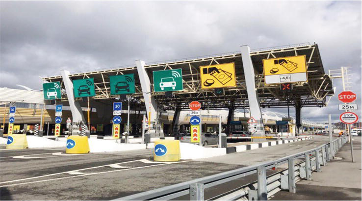
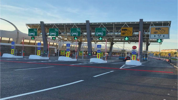
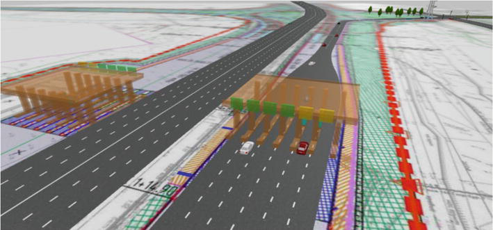
As an example, the analysis of the TP Bogatyrskiy Ave./Planernaya Str., located at the exit from the WHSD toll road to the Primorsky District of St. Petersburg (Figure 1) simulation model is done.

Figure 1.

General view of the Bogatyrskiy Ave./Planernaya Str. TP.

The toll road uses an open-type barrier tolling system. The Primorsky district has the first largest population in the city and also has active daily labor correspondence. Since the launch of the adjacent toll road section in 2016, there has been systematic congestion at this toll road due to the insufficient capacity of the toll lanes at the TP. The configuration of this TP has six toll lanes, four of which operate in automatic mode and provide electronic toll collection (ETC) using onboard units (hereinafter referred to as OBU). The toll mode provides for nonstop passing through the lanes at a maximum speed of 30 km/h. The remaining two lanes are in manual mode and allow cash or bank card payments to be made to the cashier-operator. The traffic model affects only the TP at the exit to the Primorsky District and does not affect the traffic on the main direction of the toll road and on the return to the road from the district.

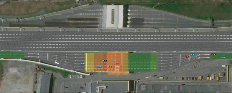
The simulation model (hereinafter referred to as SM) has been developed in AnyLogic software using traffic and process modeling libraries. The resulting TP model is presented in Figure 2.

Figure 2.

SM of the Bogatyrskiy Ave./Planernaya Str. TP.

The SM of the TP allows the following traffic flow parameters to be taken into account:

• The intensity of traffic at the TP;

• The composition of traffic;

• Distribution of vehicles by the method of payment;

• Time of service in the automated lane;

• Time of service in the cash payment lane;

• Additional parameters (user behavior and tag failure).

3.2 Queuing analysis

The data for the SM, including data on intensity, traffic composition, distribution of payment methods, and service time, are obtained from video data from the Northern Capital Highway LLC website [32]. The number of vehicles passing through for 10–15 minutes was counted and the results were converted to the number of vehicles per hour. Corresponding calculations were made for all days of the week and time intervals of 24 astronomical hours. The results obtained for the same day of the week and time of day were averaged. There were no significant traffic fluctuations related to major urban cultural events during the time period in question, which could lead to significant changes in the weekly traffic cycle. There are no major logistics centers in the Primorsky district and heavy vehicle traffic is prohibited at the TP, allowing only passenger cars to be taken into account in the SM. The specified length of passenger cars in the model is 5 meters. Distribution of vehicles by payment method for this TP is 80% ETC transactions and 20% manual toll collection. It is assumed that manual toll lanes service time is triangularly distributed with a mean value of 20 (for contactless bank card payments), min of 7 (for ETC), and max value of 45 (for contact bank cards and cash payments) seconds.

An additional parameter of user behavior—tag failure—has been introduced into the model which affects the capacity of the ETC lanes. The “tag failure” parameter takes into account the probability of transponder failure (5%) when passing through ETC lanes in case the vehicle has not been read in the entry antenna, is incorrectly attached, or has a negative balance, that is, is not accepted for payment. It is assumed that tag failure time is also triangularly distributed with a mean value of 7 (in case of wrong OBU fixing), min of 3 (in case of second antenna reading), and max value of 60 (in case of negative balance) seconds.

An additional feature of the TP under study is the bottleneck at the exit of the main road (only two lanes), the six lanes (the TP itself), and the joining of the six lanes back to two lanes after the TP exit. This feature allows one to consider the whole of the TP as a “bottleneck” slowing down the speed of traffic and to estimate the time it takes to pass the section from the toll road exit to the point where the six lanes are connected back to two lanes.

The analysis of the daily traffic volume of the TP allows us to determine the distribution of user service times on the toll lanes as well as to assess the possibility of congestion occurring during the day on a weekly cycle.

3.3 Traffic intensity

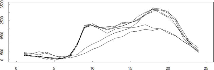
Figure 3 shows the graph of observed traffic intensity at Bogatyrsky Ave./Planernaya Str. TP by days of the week from 0:00 to 24:00 (intensity was calculated in number of vehicles/h).

Figure 3.

Traffic intensity at the Bogatyrsky Ave./Planernaya Str. TP by days of the week from 0:00 to 24:00 (intensity was calculated in number of vehicles/h).

Figure 3 shows seven schedules (five for weekdays and two for weekends). Weekdays are characterized by higher traffic volumes than weekends. The weekday schedules do not differ much from each other. The peak weekday intensities for the TP fall in the evening rush hour and correspond to work-home correspondences.

3.4 Analysis of toll plaza simulation model

As can be seen from Figure 3, the traffic volumes at the TP vary between 60 and 3140 vehicles/h, depending on the day of the week and time of day. We will be interested in the answers to the following questions:

• At what traffic intensity will traffic congestion be generated in front of the entrance to the TP?

• How does the intensity of incoming traffic affect the distribution of vehicle service time at the TP?

In contrast to classical mass-transit theory schemes, we define service time as the time it takes for a vehicle to cross a TP from the exit point of the main road (the exit has only two lanes) to the point after the TP, where the six lanes of the TP rejoin the two-lane road (see Figure 2).

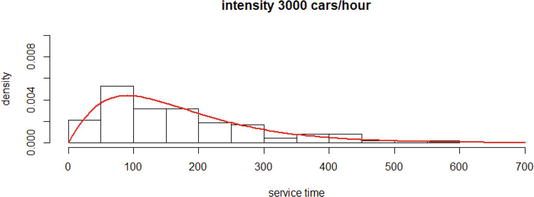
A number of experiments have been carried out on the SM of the TP. The distribution of service time was studied, with input flow rates from 250 to 3250 vehicles/h, in steps of 250. The occurrence of congestion is considered to be the appearance of a queue of vehicles beyond the entrance area of the TP. The results of the experiments show that congestion starts to form when the traffic intensity is higher than 1010 vehicles/h. Before this intensity is reached, the empirical service time distribution (vehicle passing through the TP zone) is an easily separable mixture of two distributions that approximate the gamma distribution well, each corresponding to vehicle passing time through either the ETC lane or the cash payment lane. Since perturbations in the form of user behavior effects are added to the model, the gamma law of the service time distribution seems to be quite expected, as being more general with respect to the Erlang distribution (see more details in the article by Talavirya A.Yu., Laskin M.B. [33]). Figure 4 shows the distribution of service times (section traversal) for a traffic volume of 3000 vehicles/h.

Figure 4.

Empirical distribution of service times at an input flow rate of 3000 vehicles/h.

Parameters of the gamma distribution shape = 2.1510, rate = 0.0126. The result of the Kolmogorov-Smirnov test for consistency of the empirical distribution with the model distribution with the specified parameters: p-value = 0.7748. At this traffic intensity, the “tag failure” effect appears: there are many vehicles, user behavior and tag failures affect the time for other vehicles to pass the TP, as a consequence, the whole TP starts to operate as a single mass service machine, the mixture of service time distributions at different payment methods is indivisible. At such high intensity, the service time distribution obeys the gamma distribution law with parameters where the distribution has significant left-hand asymmetry. Table 1 presents the parameters of the gamma law distribution of the service time at high input flow intensities.

Intensity	Gamma distribution parameters			Expectation	Mode
	shape	rate	p-value
1250 vehicles/h	1.521	0.0132	0.0617	115	39
1500 vehicles/h	2.0381	0.0127	0.3758	161	82
1750 vehicles/h	1.9516	0.0137	0.3035	142	69
2000 vehicles/h	2.533	0.0149	0.1739	170	103
2250 vehicles/h	2.5919	0.0135	0.8186	192	118
2500 vehicles/h	2.2586	0.0109	0.6657	207	115
2750 vehicles/h	2.2658	0.0147	0.7156	154	86
3000 vehicles/h	2.1511	0.0126	0.7748	170	91
3250 vehicles/h	2.2402	0.0133	0.2608	169	93

Table 1.

Parameters of the gamma law distribution of the service time at high input flow intensities.

At high input flow rates, in an evolving queue environment, the mathematical expectation of the service time is significantly different from the most probable service time.

3.5 Determining the queue length when passing through a TP

When managing traffic on a toll road, the most practical relevance for the road operator is when traffic congestion occurs when entering the TP zone. In the context of congestion, the TP’s indicators considered are:

• Number of vehicles in queue and length of queue;

• The waiting time for a vehicle to cross the line of entry into the TP area.

The following assumptions were used in the consideration of these indicators:

1. The TP area is considered to be the stretch of road that includes the TP, 135 meters of roadway before entering the TP and 150 meters after exiting the TP, that is, the entire stretch of road near the TP that is widened compared to the main two-lane road;

2. The queue of vehicles is considered to be a hoarding located in front of the line of approach to the TP, the volume of the hoarding is unlimited;

3. Queuing is defined as vehicles in front of the line of approach to the TP zone moving at a speed close to zero with a minimum distance between vehicles in heavy traffic. Provided the intensity of input and output flows is approximately equal, queue formation is of random nature, the queue can form and disappear. As the intensity of incoming traffic increases and the capacity of the TP is reached, the queue begins to increase, so we consider the queue formed if the last 135 meters before the line of entrance to the TP zone is occupied by vehicles;

4. Vehicles can only leave the queue by moving forward through the TP, there is no other way to leave the queue;

5. The queue starts to form when the intensity of incoming traffic reaches a certain threshold (for the given TP and its lanes configuration) value ${\lambda }^{\ast }$;

6. The exit flow is assumed to be stationary Poisson (with constant intensity ${\lambda }^{\ast }$) as long as there is a queue in front of the TP zone, the intensity of the exit flow is assumed to be equal to the intensity of vehicles crossing the end line of the TP zone;

7. The inlet flow is stationary Poisson (with constant intensity $\lambda$) or non-stationary (with variable intensity $\lambda \left(t\right)$).

3.6 The length of the queue

Let $X$ be a random variable, the number of vehicles leaving the TP zone per unit time, distributed according to the Poisson distribution with parameter ${\lambda }^{\ast }$, that is

$$P\left(X=m\right)=\frac{{{\lambda }^{\ast }}^m}{m!}{e}^{-{\lambda }^{\ast }}$$E1

while $Y$ is a random variable, the number of vehicles arriving at the start of the queue, per time unit, distributed according to the Poisson distribution with parameter $\lambda$, that is

$$P\left(Y=n\right)=\frac{{\lambda }^n}{n!}{e}^{-\lambda }$$E2

then $V=Y-X$ is also a discrete random variable and its distribution law is given by the discrete function

$$f\left(k,\lambda ,{\lambda }^{\ast }\right)=P\left(V=k\right)=e^{-\left(\lambda +{\lambda }^{\ast }\right)}{\left(\frac{\lambda }{{\lambda }^{\ast }}\right)}^{\frac{k}{2}}{I}_{\left|k\right|}\left(2\sqrt{\lambda \times {\lambda }^{\ast }}\right).$$E3

where $I_{\left|k\right|}\left(x\right)$ is a modified Bessel function of the first kind, at $k=0,\pm 1,\pm 2,\dots ,\pm \infty$. Such a distribution is obtained by John Gordon Skellam [34]. Then (a detailed description is given in paper [33]):

$$f\left(k,\lambda ,{\lambda }^{\ast }\right)=P\left(V=k\right)=e^{-\left(\lambda +{\lambda }^{\ast }\right)}\times \sum _{m=0}^{\infty }\frac{1}{\mathrm{m}!\mathrm{\Gamma }\left(\mathrm{m}+|\mathrm{k}|+1\right)}{\lambda }^{m+\mid k\mid }\times {{\lambda }^{\ast }}^m$$E4

Main characteristics of the random variable $V$: $E\left(V\right)=\mathrm{\lambda }-{\mathrm{\lambda }}^{\ast }$, the variance of $V$:$D\left(V\right)=\lambda +{\lambda }^{\ast }$, standard deviation $\sigma \left(V\right)=\sqrt{\lambda +{\lambda }^{\ast }}$, coefficient of asymmetry:

$${\gamma }_1=\frac{\lambda -{\lambda }^{\ast }}{{\left(\lambda +{\lambda }^{\ast }\right)}^{\frac{3}{2}}}$$E5

Obviously, this distribution is symmetric only in the case of $\lambda ={\lambda }^{\ast }$.

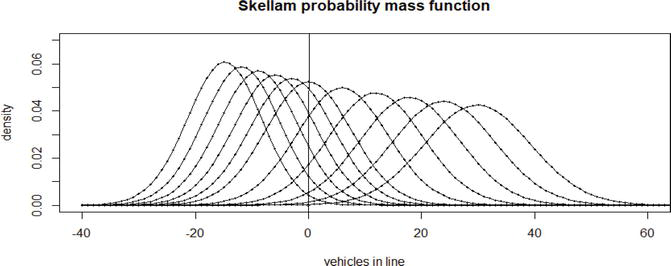
Figure 5 shows the Skellam distribution probability functions (the probabilities are defined for integer values of $k$) for different values of the parameters $\lambda ,{\lambda }^{\ast }$.

Figure 5.

Examples of Skellam distribution probability mass functions for different input-output ratios. When $\lambda$≤${\lambda }^{\ast }$ the maximum (mode) is less than zero, when $\lambda$≥${\lambda }^{\ast }$ the maximums are greater than zero.

${\lambda }^{\ast }=29.17$,

$\lambda =14.17;17.17;20.17;23.17;26.17;29.17;35.17;41.17;47.17;53.17;59.17$,

The intensities are given as vehicles/minute (14.17 corresponds to an intensity of 850 vehicles/h, 59.17 corresponds to an intensity of 3550 vehicles/h). It is obvious from Figure 5 that:

• when $\lambda$=${\lambda }^{\ast }$, the probability of queue existence is 0.5, the probability of its absence is also 0.5;

• when $\lambda$˂${\lambda }^{\ast }$the probability of queue existence is less than 0.5, it is positive and asymptotically tends to 0 when $\lambda \to 0$;

• when $\lambda$>${\lambda }^{\ast }$ the probability of queueing is greater than 0.5 and asymptotically tends to 1 when $\lambda \to +\infty$.

The length of the queue $V^{\ast }\left(t_0,\tau \right)$, formed during the time interval $\left[t_0,t_0+\tau \right]$ at variable input intensity $\lambda \left(t\right)$ will be a discrete random variable with a distribution law (see [33] for details):

$$\left\{\begin{array}{c}P\left(V^{\ast }=0\right)=e^{-\left(\mathrm{\Lambda }\left(t_0,\tau \right)+{\lambda }^{\ast }\tau \right)}\sum _{k=0}^{-\infty }{\left(\frac{\mathrm{\Lambda }\left(t_0,\tau \right)}{{\lambda }^{\ast }\tau }\right)}^{\frac{k}{2}}{I}_{\mid k\mid }\left(2\sqrt{\mathrm{\Lambda }\left(t_0,\tau \right)\times {\lambda }^{\ast }\tau }\right),k\le 0,k\in Z\\ P\left(V^{\ast }=k\right)=e^{-\left(\mathrm{\Lambda }\left(t_0,\tau \right)+{\lambda }^{\ast }\tau \right)}{\left(\frac{\mathrm{\Lambda }\left(t_0,\tau \right)}{{\lambda }^{\ast }\tau }\right)}^{\frac{k}{2}}{I}_{\mid k\mid }\left(2\sqrt{\mathrm{\Lambda }\left(t_0,\tau \right)\times {\lambda }^{\ast }\tau }\right),k>0,k\in Z\end{array}\right.$$E6

where $\mathrm{\Lambda }\left(t_0,\tau \right)=\underset{t_0}{\overset{t_0+\tau }{\int }}\lambda \left(t\right)\mathit{dt}$, and $t_0$ means the moment the queue starts to form.

The standard library function of the statistical package R can be used to calculate the values of the Bessel functions.

Table 2 shows the calculated values of the mathematical expectation and the most probable value of the queue length occurring per unit time for the TP under consideration. The calculated values for output flow intensity ${\lambda }^{\ast }=29.17$ highlighted in bold in Tables 2–4.

Input intensity vehicles/min.	Queue existence probability	Mean	Mode	Skewness
14.17	0.01	0.022	0.000	−0.05
17.17	0.04	0.100	0.000	−0.04
20.17	0.11	0.324	0.000	−0.03
23.17	0.22	0.817	0.000	−0.02
26.17	0.37	1.699	0.000	−0.01
29.17	0.50	3.040	0.000	0.00
35.17	0.79	7.048	6.000	0.01
41.17	0.93	12.281	12.000	0.02
47.17	0.98	18.056	18.000	0.03
53.17	0.99	24.010	24.000	0.03
59.17	1.00	30.002	30.000	0.04

Table 2.

Average queue length, most probable queue length, probability of queue occurrence, coefficient of asymmetry of queue length distribution formed per unit time at output flow intensity ${\lambda }^{\ast }=29.17$, and input flow intensities $\lambda =14.17;17.17;20.17;23.17;26.17;29.17;35.17;41.17;47.17;53.17;59.17$.

3.7 Waiting time in the queue

As before, $X\in \mathit{\text{Pois}}\left({\mathrm{\lambda }}^{\ast }\right)$ is a random variable, the number of vehicles leaving the TP zone per unit time, and $Y\in \mathit{\text{Pois}}\left(\mathrm{\lambda }\right)$ is a random variable, the number of vehicles arriving at the start of the queue per unit time. Then, $X_t$ is the number of vehicles leaving the TP zone in time t is also a random variable and $X_t\in \mathit{\text{Pois}}\left({\mathrm{\lambda }}^{\ast }t\right).$ It can be shown (see details in [33]) that the distribution density of the random variable T, the time in which all the vehicles arrive at the beginning of the queue per unit time (with intensity $\lambda$), with the intensity of outgoing flow ${\lambda }^{\ast }$ will leave the queue, can be written as

$$f^{\ast }\left(0,\lambda ,{\lambda }^{\ast }t\right)={\lambda }^{\ast }f\left(0,\lambda ,{\lambda }^{\ast }t\right)={\lambda }^{\ast }\times e^{-\left(\lambda +{\lambda }^{\ast }t\right)}\times I_0\left(2\sqrt{{\mathit{\lambda \lambda }}^{\ast }t}\right)$$E7

Mathematical expectation, variance, and standard deviation of the value T (waiting time in the queue of vehicles arriving at the beginning of a unit time interval):

$$E\left(T\right)=\frac{\lambda +1}{{\mathrm{\lambda }}^{\ast }},D=\frac{\lambda +1}{{{\mathrm{\lambda }}^{\ast }}^2},\mathrm{\sigma }=\frac{\sqrt{\lambda +1}}{{\mathrm{\lambda }}^{\ast }}$$E8

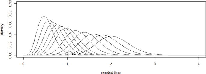
Figure 6 shows the distribution functions of the random variable T, with different ratios of $\lambda$ and ${\lambda }^{\ast }:{\lambda }^{\ast }=29.17$,

Figure 6.

Distribution density of the random variable T, with ${\lambda }^{\ast }=29.17$ and $\lambda$ ranging from 14.17 to 59.17 = vehicles/min (850 to 3555 vehicles/h).

$\lambda =14.17;17.17;20.17;23.17;26.17;29.17;35.17;41.17;47.17;53.17;59.17$.

Numerical characteristics of time distribution T can be obtained either by calculation (e.g., expected value, variance, standard deviation) or by simulation in R statistical package. Table 3 shows the values of the mathematical expectation and the most probable value of T obtained by modeling in R and the mathematical expectation, variance, and standard deviation obtained by Eq. (8).

Input intensity vehicles/min.	R simulated values		Calculated values
	Mean time	Modal time	Mean time	Variance	Standard deviation
14.17	0.520	0.480	0.520	0.02	0.13
17.17	0.623	0.580	0.623	0.02	0.15
20.17	0.726	0.680	0.726	0.02	0.16
23.17	0.826	0.790	0.829	0.03	0.17
26.17	0.931	0.890	0.931	0.03	0.18
29.17	1.034	0.990	1.034	0.04	0.19
35.17	1.240	1.200	1.240	0.04	0.21
41.17	1.446	1.400	1.446	0.05	0.22
47.17	1.651	1.610	1.651	0.06	0.24
53.17	1.857	1.820	1.857	0.06	0.25
59.17	2.063	2.063	2.063	0.07	0.27

Table 3.

Mathematical expectation, the modal value of T obtained by modeling in R, and mathematical expectation, variance, and standard deviation obtained by Eq. (8).

3.8 Changing the dimensionality of intensities and time scales

When changing the time scale, it should be taken into account, that in Eqs. (6) and (7) at an increase of values of the exponent argument and the modified Bessel function (first kind, order 0) at numerical calculations even within really existing values of intensities and the time intervals of interest, the machine zero is quickly formed. Therefore, in the calculations, it is better to change the ratios of intensities and time scales so that the function arguments in Eqs. (6) and (7) allow for obtaining numerical values. Suppose that we want to obtain an estimate of queue waiting time in hours, knowing the intensity expressed in TC per hour. The intensities ${\lambda }^{\ast }=29.17$, $\lambda =14.17;17.17;20.17;23.17;26.17;29.17;35.17;41.17;47.17;53.17;59.17$, previously dimensioned in TC per minute are converted to TC per hour: ${\lambda }^{\ast }=1750$, $\lambda =850;1030;1210;1390;1570;1750;2110;2470;2830;3190;3550$. Such dimensionality is also not yet suitable for calculating exponents and values of Bessel functions. On the basis of actual intensities on the considered road, it seems reasonable to consider hourly intensities in hundreds of vehicles per hour (${\lambda }^{\ast }=17.50$, $\lambda =8.50;10.30;12.10;13.90;15.70;17.50;21.10;24.70;28.30;31.90;35.50$), the time unit is 1 hour. We obtain a similar figure and parameters of time distribution laws, but already in hours (Table 4).

Input intensity 100 vehicles/h	R simulated values		Calculated values
	Mean time (hour)	Modal time (hour)	Mean time (hour)	Variance	Standard deviation (hour)
8.5	0.54	0.47	0.54	0.03	0.18
10.3	0.65	0.57	0.65	0.04	0.19
12.1	0.75	0.67	0.75	0.04	0.21
13.9	0.85	0.78	0.85	0.05	0.22
15.7	0.95	0.88	0.95	0.05	0.23
17.5	1.06	0.98	1.06	0.06	0.25
21.1	1.26	1.19	1.26	0.07	0.27
24.7	1.47	1.39	1.47	0.08	0.29
28.3	1.67	1.60	1.67	0.10	0.31
31.9	1.88	1.80	1.88	0.11	0.33
35.5	2.09	2.01	2.09	0.12	0.35

Table 4.

Mathematical expectation, modal value of T obtained by modeling in R, and mathematical expectation, variance, and standard deviation obtained by Eq. (8) in hours.

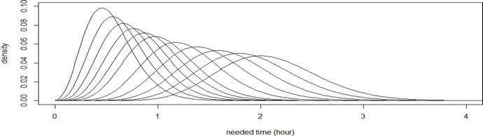
Figure 7 shows the distribution functions of the random variable T, with different ratios of $\lambda$ and ${\lambda }^{\ast }:{\lambda }^{\ast }=17.5$, $\lambda =10.3;12.1;13.9;15.7;17.5;21.1;24.7;28.3;31.9;35.5$.

Figure 7.

Distribution density of the random variable T, with ${\lambda }^{\ast }=17.5$ (100 vehicles/h) and $\lambda$ ranging from 8.50 to 35.55 (100 vehicles/h).

The asymmetry of the obtained distribution laws is insignificant (the modal value differs from the mean between 3.6% and 13.4%), but the standard deviation is rather large.

When the input intensity is variable ($\lambda =\lambda \left(h\right))$, h —time of day), we consider the input intensity parameter as $\Lambda \left(h_0,\tau \right)=\underset{h_0}{\overset{h_0+\tau }{\int }}\lambda \left(h\right)\mathit{dh}$, …$h_0$— the time (time of day) of the onset of road congestion.

In Laskin et al. [35], it is shown that the daily intensities given in Figure 3 can be well approximated by the first n terms of the trigonometric series. This model has been applied to the study of queue lengths over the course of a day.

When examining the queue length and waiting time for vehicles in the queue before entering the TP zone, we consider the accumulated intensity as

$$\Lambda \left(h_0,\tau \right)=\underset{h_0}{\overset{h_0+\tau }{\int }}\lambda \left(h\right)\mathit{dh}$$E9

where $h_0$ is the moment at which a period of time $\tau$ of length begins to be counted.

We estimate the queue length by the mean value $E\left(V\right)=\Lambda \left(h_0,\tau \right)-{\lambda }^{\ast }\tau$ with standard deviation $\sigma \left(V\right)=\sqrt{\Lambda \left(h_0,\tau \right)+{\lambda }^{\ast }\tau }$. We estimate the waiting time in queue θ by the mean $E\left(\theta \right)=E\left(T\right)\ast \tau -\tau =\frac{\Lambda \left(h_0,\tau \right)+1}{{\lambda }^{\ast }\tau }\times \tau -\tau =\frac{\Lambda \left(h_0,\tau \right)-{\lambda }^{\ast }+1}{{\lambda }^{\ast }}$ with standard deviation $\sigma \left(\theta \right)=\sigma \left(T\right)=\frac{\sqrt{\Lambda \left(h_0,\tau \right)+1}}{{\lambda }^{\ast }\tau }$.

The corresponding calculations were performed in the R statistical package environment, for the following input and output flows and TP parameters:

• An example of changing input intensity observed during October 2019 was chosen for modeling (shown in Figure 2); a trigonometric series was used for approximation, similar to the article by Laskin et al. [35];

• The outbound flow intensity is considered to be equal to the minimum inbound flow intensity at which stable traffic congestion is formed when entering the TP zone; it was determined by simulation methods under the following parameters of six toll lanes operation mode: four lanes with automatic transponder signal reading, two lanes providing cash payment (the second lane is mandatory as backup), readout failures (user behavior)-5% of total number of vehicles in the flow, percentage of vehicles equipped with a transponder. The simulations with different entry flow intensities show that with these TP parameters a stable inlet congestion is formed at an entry flow intensity of 2550 vehicles/h;

• The estimation of the queue length with the distribution law $P\left(V^{\ast }\left(t_0,\tau \right)=k\right)$(6), as seen in Figure 5, depends on the ratio $\Lambda \left(h_0,\tau \right)$ and ${\lambda }^{\ast }\tau$, if these values are close, the queue can appear and disappear, but as the value $\Lambda \left(h_0,\tau \right)$increases, the probability that congestion exists increases. Therefore, under the conditions of the persistent congestion observed in the simulation, we assume the difference between $\Lambda \left(h_0,\tau \right)$ and ${\lambda }^{\ast }\tau$ to be large enough to use Eqs. (7) and (8) to estimate the average queue length and its standard deviation for the estimation judgments:

  $$E\left(V^{\ast }\right)\approx \Lambda \left(h_0,\tau \right)-{\lambda }^{\ast }\tau ,$$E10
  $$\sigma \left(V^{\ast }\right)\approx \sqrt{\Lambda \left(h_0,\tau \right)+{\lambda }^{\ast }\tau }$$E11

• The estimation of the queueing time also depends on the parameters $\Lambda \left(h_0,\tau \right)$ and ${\lambda }^{\ast }\tau$. We use the following representations for the estimated queueing time judgments:

  $$E\left(T\right)\approx \frac{\Lambda \left(h_0,\tau \right)+1}{{\lambda }^{\ast }\tau },$$E12
  $$\sigma \left(T\right)\approx \frac{\sqrt{\Lambda \left(h_0,\tau \right)+1}}{{\lambda }^{\ast }\tau }$$E13

The results are shown in Figures 8 and 9 and Table 5.

Figure 8.

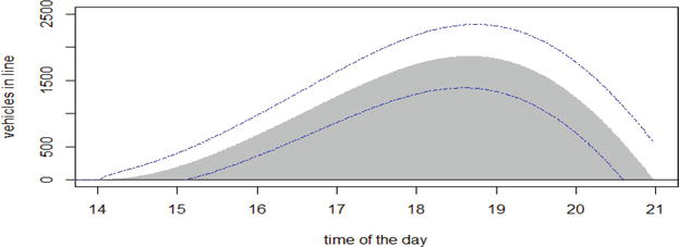
Estimation of average number of vehicles in queue during the working day. The blue line is a corridor of +/− 3σ.

Figure 9.

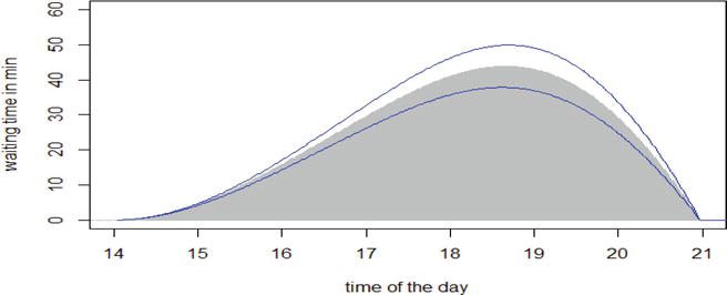
Estimation of waiting time (in minutes) for vehicles in the queue from the moment of approach to the beginning of the queue to the entrance to the TP zone, depending on the time of day when the vehicle arrived at the beginning of the queue. The blue lines show a corridor of possible deviations of +/− 3σ to the average waiting time.

Time of the day	Average queue length in vehicle	Average queue length in vehicle-3σ	Average queue length in vehicle +3σ	3-lane queue in km	4-lane queue in km	Average waiting time (min.)	Average waiting time (min.)-3σ	Average waiting time (min.) + 3σ
14:00	—	—	—	—	—	—	—	—
15:00	189	—	403	0.5	0.38	4.5	4.2	4.7
16:00	667	356	977	1.8	1.33	16.0	14.0	17.0
17:00	1250	865	1634	3.3	2.50	30.0	26.0	33.0
18:00	1739	1295	2184	4.6	3.48	41.0	36.0	46.0
18:40	1862	1385	2340	5.0	3.72	44.0	38.0	50.0
19:00	1825	1331	2320	4.9	3.65	43.0	37.0	49.0
20:00	1238	704	1772	3.3	2.48	29.0	25.0	34.0
20:30	676	126	1227	1.8	1.35	16.0	13.5	18.4
21:00	—	—	—	—	—	—	—	—

Table 5.

Time of day, average queue length in vehicles, corridor of possible deviations to average queue length +/− 3σ, estimate of average queue length in km, average waiting time in queue before entering the TP zone, and corridor of possible deviations to average waiting time +/− 3σ.

3.9 Time of existence of the queue

The queue begins to form at 843 minutes from the beginning of the day (00:00), which corresponds to the time of day 14:03.

The queue ceases to exist at 1259 minutes from the beginning of the day (00:00), which corresponds to the time of day 20:59.

Thus, a queue consisting of slow-moving vehicles on the Bogatyrsky St./Planernaya St. TP exists from 14:03 to 20:59 (2:03 PM to 8:59 PM). The queue length is permanently changing, the estimate of its average value is shown in Figure 8. The blue dotted lines show the corridor +/− 3σ for estimating the queue length.

3.10 Maximum queue length, waiting time in queue

The maximum number of vehicles in the queue is estimated at 1863 vehicles, which with a queue of four lanes (4 lanes on the main toll road to the exit to the TP), would be 3.72 km in length. The longest queue length corresponds to 1120 minutes, which corresponds to a time of day of 18:40. The range of possible changes in queue length at the time of greatest length is between 1386 and 2343 vehicles.

Table 5 shows:

1. The average queue length in vehicles;

2. Corridor of possible (+/−3σ) changes to queue length;

3. Estimation of average queue length in kilometers;

4. Average waiting time in the queue before entering the TP zone;

5. Corridor of possible changes.

There is a short (160-meter) stretch of road that has two lanes before exiting to the Bogatyrsky TP. When congestion occurs in front of the toll road, the queue exits beyond the TP zone onto the main course of the toll road, which has four lanes, so the queue length has been estimated for a queue formed of four lanes. The distance between two vehicles standing one behind the other in dense traffic is 8 meters.

The waiting time in the queue before exiting the main turn and entering the TP zone is an estimation and reflects only the case when vehicles in the flow are moving without rearrangements and are lined up, for example, in 4 lanes, when approaching the beginning of the queue. In reality, this condition is not systematically fulfilled, so the dispersion of waiting time of vehicles in the queue can increase significantly due to the actions of unruly drivers. This circumstance does not affect the waiting time of the queue.

To confirm that the calculated values of the queue length and queueing time before entering the TP zone correspond to the actual road traffic situation, we use data from the search and information mapping service Yandex.Maps for St. Petersburg. This service displays both the current traffic situation in real time and forecasted congestion length (in km) on the WHSD road section before the Bogatyrsky St./Planernaya St. TP based on statistical data. Table 6 shows the lengths of the forecasted congestion (in km) on weekdays in February 2020 due to the low traffic intensity on weekends, there is no congestion then.

Weekday/Time	Monday	Tuesday	Wednesday	Thursday	Friday
16:00	0.9	2.36	2.16	1.74	2.36
16:30	1.7	3.02	2.94	3.39	3.65
17:00	3.22	4.9	3.87	3.68	4.89
17:30	4.9	5.05	4.75	3.86	4.89
18:00	5.29	5.09	4.75	4.65	4.91
18:30	5.29	5.13	4.75	4.65	4.91
19:00	5.29	4.91	4.75	4.65	4.67
19:30	5.29	4.75	4.64	4.65	3.69
20:00	4.93	3.87	3.75	3.03	2.36
20:30	2.25	0.91	1.64	2.46	0.1
21:00	0	0.93	0	0	0
21:30	0	0	0	0	0

Table 6.

The lengths of the forecasted congestions (in km) on weekdays in February 2020, based on data from the Yandex.Map map service.

As shown in Table 6, the queue time and length during peak hours at the Bogatyrsky St./Planernaya St. TP, which were obtained for the developed simulation model, are close to the forecasted values obtained from empirical data collected by the Yandex.Maps map service.

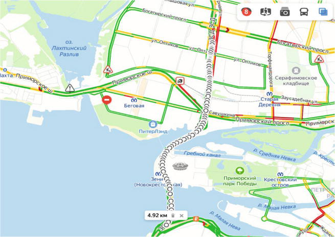
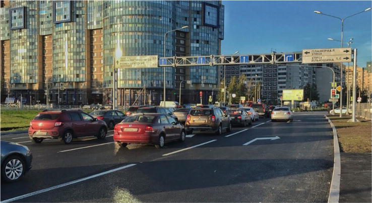
In addition, the real-time congestion information for the WHSD road section before Bogatyrsky St./Planernaya St., based on Yandex.Maps service information, was monitored during peak hours. As an example, the results from the monitoring on Thursday, January 21, 2021, at 18:30, are shown in Figure 10.

Figure 10.

Congestion (4.92 km length) on the WHSD formed during peak hours at the Bogatyrsky St./Planernaya St. TP at 18:30, 21.01.2021, according to the Yandex.Maps map service.

As shown in Figure 10, the length of the congestion, formed during rush hour on weekdays, reaches 4.92 km. The observed value is close to the obtained results of average maximum number of vehicles in the queue, indicated in Table 5.

4. Toll plaza on the main course of a toll road

4.1 Toll plaza on the main course of a toll road

In order to assess the effectiveness of the TCS for the operation of the TP on the main course of a toll road, the SM of the TP “Main course behind the Ring Road (North) towards Primorsky Ave,” located on the northern section of the WHSD, was developed. A general view of the developed SM of the TP is shown in Figure 11.

Figure 11.

The SM of the TP “Main course behind the Ring Road (North) towards Primorsky Ave.” TP zone.

The existing configuration of the TP “Main course behind the Ring Road (North) towards Primorsky Ave” has nine toll lanes, five of which operate in automatic mode, and the remaining four lanes operate in manual mode.

To assess the current performance of the named TP a SM was implemented taking into account the current configuration mode of the TCS (five automatic and four manual lanes) as well as the current share of ETC devices used by users is 91%. In order to solve the problem of forecasting the TP efficiency in the current configuration of the TCS, three additional SMs were also implemented with projected values of ETC devices used by 2022—93, 95, and 97%.

In order to solve the problem of optimizing TP efficiency, SMs with the following lane configurations has been implemented:

• A configuration with six automatic and three manual toll lanes;

• A configuration with seven automatic and two manual toll lanes.

The above models have been considered in two different modes of user behavior: 10 and 5% of the errors committed by ETC devices users when passing the automatic toll lanes.

It should be noted that a configuration with seven automatic toll lanes and two manual toll lanes is the maximum permissible for this TP. Reason: the TP must be able to provide cash and bank card payment in the TCS configuration, and a minimum of two manual lanes must be available, subject to redundancy, in case one of the lanes fails.

For each of the configurations, SMs were implemented with existing and projected ETC devices usage values. Thus, for each of the three TCS configurations, four SMs were implemented to assess changes in system performance when the ETC devices pass rates increased over a range of values of 91, 93, 95, and 97%, and user behavior error levels of 10 and 5%.

4.2 Observed traffic volume at the TP

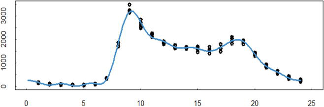
Data on intensity, traffic composition, and time of service were obtained by a visual count of passing vehicles through the TP from an online camera located on it from the road operator’s website [32] during the period from October to November 2019. On the traffic direction under study, during weekdays from Monday to Friday, the traffic intensity was observed to not exceed 3500 vehicles per hour. At weekends, the traffic flow schedule varies but also does not exceed 3500 vehicles per hour. The intensity data for the five working days of the observations is shown in Figure 12.

Figure 12.

Observed traffic volumes on weekdays and the approximating variable intensity curve at ПВП the TP “Main course behind the ring road (north) towards Primorsky Ave.” traffic—From 0:00 to 24:00 (intensity—in number of vehicles/h).

Similar to 3.8, the daily intensities shown in Figure 12 can be well approximated by the first n terms of the trigonometric series. Such a model is constructed with the first nine terms (19 coefficients) of a trigonometric series of the form. A similar pattern is observed for holidays and weekends, for which approximating functions can be constructed. As part of the study, we are interested in two questions:

1. At what intensities and parameters (fraction of ETC devices users, fraction of user behavior errors) of the incoming flow of incoming traffic will congestion be generated at the TP?

2. What measures can the operator take to reduce the risk of traffic congestion within the existing configuration of a TP consisting of nine toll lanes?

4.3 Time allocation for passing the TP zone

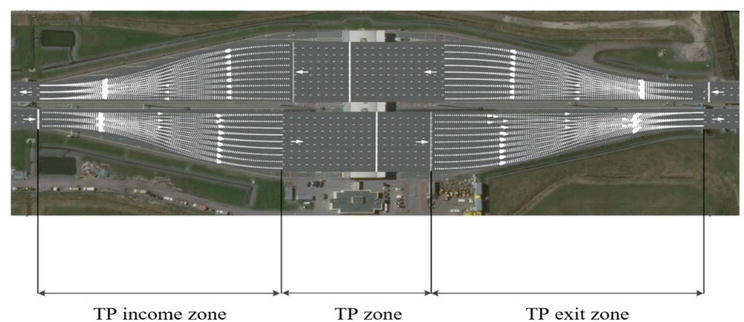
The TP zone, comprising nine toll lanes separated by safety islands, is defined as a section of toll road beginning at the approach area of the toll road when the 3-lane main course is extended and ending at the exit area of the toll road where the nine toll lanes are converted back to three lanes. We separate the concepts of the service time directly at the toll lane (which would be the baseline when applying classical mass service theory) and the driving time to the TP zone. In this case, we are interested in the time it takes for a vehicle to travel the entire stretch of road from the TP entrance area to the TP exit area. We assume that congestion occurs in situations where vehicles cannot cross the line of division of three lanes into nine and have to queue up to this line.

The distribution of service times for manual and automatic toll lanes is specified in the SM parameters. The study of traffic at different intensities of the incoming traffic has shown that at low intensities the distribution of service times is a mixture of split distribution laws, obviously corresponding to the passage of vehicles through manual and automatic toll lanes. From the practical point of view, these cases are not of interest, as the TP can handle the load.

At high intensity, the distribution of TP driving times at manual and automatic toll lanes is an indistinguishable mix of distributions. At high intensities, the role of user behavior errors increases, leading to significant flow changes at the TP zone and causing interference to other road users. The distribution of TP driving The TP Zone, comprising nine toll lanes separated by safety islands, is defined as a section of toll road beginning at the approach area of the toll road when the 3-lane main course is extended and ending at the exit area of the toll road where the nine toll lanes are converted back to three lanes. We separate the concepts of the service time directly at the toll lane (which would be the baseline when applying classical mass service theory) and the travel time to the TP zone. In this case, we are interested in the time it takes for a vehicle to travel the entire stretch of road from the TP entrance area to the TP exit area. We assume that congestion occurs in situations where vehicles cannot cross the line of division of three lanes into nine and have to queue up to this line.

The distribution of service times for manual and automatic toll lanes is specified in the SM parameters. The study of traffic at different intensities of the incoming traffic has shown that at low intensities the distribution of service times is a mixture of split distribution laws, obviously corresponding to the passage of vehicles through manual and automatic toll lanes. From the practical point of view, these cases are not of interest, as the TP can handle the load.

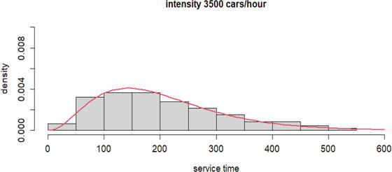
At high intensity, the distribution of TP driving times at manual and automatic toll lanes is an indistinguishable mix of distributions. At high intensities, the role of user behavior errors increases, leading to significant flow changes at the TP zone and causing interference to other road users. The distribution of TP driving times in these cases is well approximated by a gamma distribution law (shown in Figure 13).

Figure 13.

Service time distribution with an input flow of 3500 vehicles/h, TCS configuration: Four manual and five automatic lanes, 91% transponders in the flow, and 10% user error rate. The red line is gamma density law distribution with parameters shape = 3.2821, rate = 0.016, p-value of Kolmogorov-Smirnov test −0.99.

The mathematical expectation of a random variable distributed in accordance to Gamma distribution $\mathit{\text{Gamma}}\left(k,\theta \right)$ is $k\times \theta$, and the modal (most likely) value is $\left(k-1\right)\times \theta$, where $k$ is a shape parameter, and $\theta =\frac{1}{\mathit{\text{rate}}}$.

When congestion occurs and the income flow intensity continues to increase, the parameters of the approximating gamma laws can vary, but the estimates of the mean TP zone driving time do not change significantly when the inlet intensity increases when the congestion is already in place.

Before the congestion occurred, the average time to cross the TP zone was calculated as a weighted average of the average TP zone crossing times for automatic (0.91) and manual lanes (0.09). After the occurrence of congestion, the average TP zone driving time was calculated as the mathematical expectation of the approximating density of the gamma law distribution. In the case under consideration, congestion occurs at an input flow rate of 1650 vehicles per hour if the user error rate is assumed to be 10% and at a rate of 3200 vehicles per hour if the user error rate is assumed to be 5%, that is, halving the user error rate significantly increases the capacity of the entire TP. If congestion has already occurred, the average driving time through the TP stabilizes and ceases to increase (this does not include waiting in line before entering the TP), and user error rates are no longer as important.

If congestion has already occurred and the income traffic intensity continues to increase, the congestion cannot be relieved until the inbound traffic intensity decreases. The maximum traffic intensity observed at this TP did not exceed the value of 3500 vehicles per hour. Already in the current situation, congestion at the TP is generated with 1500–1600 vehicles per hour (see Figure 12), that is, during peak hours.

With increasing traffic flows, the frequency of traffic congestion and queue lengths will only increase. The natural way to prevent congestion seems to be:

• Increasing the share of ETC devices in traffic flow;

• Reconfiguring TPs by increasing the number of automatic toll lanes;

• Road operator’s implementation of a set of information measures aimed at reducing user behavior when using ETC devices to pass through the automatic toll lanes.

Tables 7 and 8 show the simulation results for different intensities, number of automatic lanes, shares of ETC devices users in the flow, and error levels of user behavior.

Traffic intensity	Uses behavior (%)	TP configuration	ETC proportion (%)	Gamma distribution parameters			Expectation	Mode	Congestion at the entrance
				Shape	rate	p-value
1600	10	4 manual + 5 ETC	91	2.9375	0.0277	0.086	106	70	No
1650	10	4 manual + 5 ETC	91	1.8637	0.0146	0.538	128	59	Yes
3500	10	4 manual + 5 ETC	91	3.2064	0.0158	0.738	203	139	Yes
1650	10	4 manual + 5 ETC	93	3.2898	0.0380	0.233	87	60	No
1700	10	4 manual + 5 ETC	93	3.0552	0.0215	0.735	142	95	No
3500	10	4 manual + 5 ETC	93	3.3242	0.0168	0.322	198	139	No
1700	10	4 manual + 5 ETC	95	2.5553	0.0248	0.077	103	63	Yes
1750	10	4 manual + 5 ETC	95	2.3994	0.0221	0.067	109	63	Yes
3500	10	4 manual + 5 ETC	95	3.5340	0.0187	0.749	189	136	Yes
1500	10	4 manual + 5 ETC	97	2.4283	0.0219	0.017	111	65	No
1550	10	4 manual + 5 ETC	97	2.0937	0.0111	0.465	189	99	No
3500	10	4 manual + 5 ETC	97	4.3142	0.0237	0.680	182	140	No
1600	10	3 manual + 6 ETC	91	2.2374	0.0212	0.630	106	58	No
1650	10	3 manual + 6 ETC	91	2.4938	0.0237	0.069	105	63	No
3500	10	3 manual + 6 ETC	91	2.9655	0.0157	0.781	188	125	Yes
1550	10	3 manual + 6 ETC	93	2.9357	0.0425	0.160	69	46	Yes
1600	10	3 manual + 6 ETC	93	2.0936	0.0178	0.391	118	62	Yes
3500	10	3 manual + 6 ETC	93	3.0855	0.0177	0.507	174	118	Yes
1500	10	3 manual + 6 ETC	95	2.5761	0.0350	0.035	74	45	No
1550	10	3 manual + 6 ETC	95	2.6170	0.0267	0.155	98	61	Yes
3500	10	3 manual + 6 ETC	95	3.2146	0.0200	0.960	161	111	Yes
1450	10	3 manual + 6 ETC	97	3.5774	0.0502	0.037	71	51	No
1500	10	3 manual + 6 ETC	97	2.6137	0.0152	0.694	172	106	Yes
3500	10	3 manual + 6 ETC	97	2.7377	0.0159	0.623	172	109	Yes
1800	10	2 manual + 7 ETC	91	2.4565	0.0225	0.204	109	65	No
1900	10	2 manual + 7 ETC	91	1.8873	0.0131	0.082	144	68	Yes
2000	10	2 manual + 7 ETC	91	2.3521	0.0199	0.109	118	68	Yes
2100	10	2 manual + 7 ETC	91	2.5431	0.0155	0.591	164	99	Yes
2500	10	2 manual + 7 ETC	91	3.0474	0.0182	0.705	168	113	Yes
3000	10	2 manual + 7 ETC	91	3.0389	0.0154	0.759	198	133	Yes
3500	10	2 manual + 7 ETC	91	2.5843	0.0151	0.538	171	105	Yes
1650	10	2 manual + 7 ETC	93	4.7607	0.0881	0.155	54	43	No
1700	10	2 manual + 7 ETC	93	1.7889	0.0168	0.061	106	47	Yes
3500	10	2 manual + 7 ETC	93	3.3748	0.0167	0.810	202	142	Yes
1650	10	2 manual + 7 ETC	95	2.7946	0.0439	0.126	64	41	No
1700	10	2 manual + 7 ETC	95	2.6577	0.0278	0.085	96	60	Yes
3500	10	2 manual + 7 ETC	95	3.6861	0.0259	0.583	142	104	Yes
1450	10	2 manual + 7 ETC	97	4.6575	0.0795	0.003	59	46	No
1500	10	2 manual + 7 ETC	97	1.5720	0.0113	0.099	139	51	Yes
3500	10	2 manual + 7 ETC	97	3.1908	0.0196	1.000	163	112	Yes

Table 7.

Simulation results for control flow parameters and lane configurations at a user behavior error rate of 10%.

Traffic intensity	Uses behavior (%)	TP configuration	ETC proportion (%)	Gamma distribution parameters			Expectation	Mode	Congestion at the entrance
				Shape	rate	p-value
3150	5	4 manual + 5 ETC	91	3.4468	0.0212	0.956	163	116	No
3200	5	4 manual + 5 ETC	91	3.6123	0.0222	0.833	163	118	Yes
5000	5	4 manual + 5 ETC	91	3.5510	0.0215	0.929	165	119	Yes
3000	5	4 manual + 5 ETC	93	3.5311	0.0217	0.616	162	116	No
5000	5	4 manual + 5 ETC	93	3.4889	0.0216	0.968	162	115	No
3000	5	4 manual + 5 ETC	95	3.2896	0.0202	0.990	163	113	No
5000	5	4 manual + 5 ETC	95	3.6504	0.0220	0.738	166	121	No
3000	5	4 manual + 5 ETC	97	7.3778	0.0852	0.893	87	75	No
5000	5	4 manual + 5 ETC	97	6.0563	0.0458	0.983	132	110	No
3000	5	3 manual + 6 ETC	91	2.6839	0.0260	0.057	103	65	No
5000	5	3 manual + 6 ETC	91	3.0190	0.0225	0.376	134	90	No
3000	5	3 manual + 6 ETC	93	4.5039	0.0524	0.176	86	67	No
5000	5	3 manual + 6 ETC	93	3.2217	0.0305	0.185	106	73	No
3000	5	3 manual + 6 ETC	95	3.6269	0.0365	0.188	99	72	No
5000	5	3 manual + 6 ETC	95	6.4878	0.0705	0.706	92	78	No
3000	5	3 manual + 6 ETC	97	10.3129	0.1499	0.319	69	62	No
5000	5	3 manual + 6 ETC	97	4.3676	0.0379	0.896	115	89	No
3000	5	2 manual + 7 ETC	91	3.3526	0.0397	0.061	84	59	No
5000	5	2 manual + 7 ETC	91	2.5611	0.0189	0.096	135	82	No
3000	5	2 manual + 7 ETC	93	5.6887	0.0710	0.051	80	66	No
5000	5	2 manual + 7 ETC	93	3.4629	0.0320	0.143	108	77	No
3000	5	2 manual + 7 ETC	95	9.4472	0.1353	0.121	70	62	No
5000	5	2 manual + 7 ETC	95	5.1386	0.0555	0.411	93	75	No
3000	5	2 manual + 7 ETC	97	5.2843	0.0660	0.400	80	65	No
5000	5	2 manual + 7 ETC	97	4.5880	0.0435	0.309	105	82	No

Table 8.

Simulation results for control flow parameters and toll lanes configurations at a user behavior error rate of 5%.

Tables 7 and 8 show that.

• Increasing the proportion of ETC devices in the TP flow, at a user behavior error level of 10% has almost no effect on the intensity threshold at which congestion begins to form (thresholds 1650, 1700, 1750, 1550), the time to pass the TP zone in this case does not change significantly;

• Configuring TP to increase the number of lanes and increase the proportion of ETC devices users with a 10% level of user error marginally affects the threshold intensity at which congestion begins to build and the time to cross the TP, congestions still begin to build at vehicle throughput rates of 1500–1750 vehicles per hour;

• Significant increase of threshold intensity at which congestion is formed is to reduce user behavior error rate to 5% with some reduction in tailing time, but the risk of short-term congestion at the exit of the TP zone. When there is a large number of vehicles in the queue, high speed of automatic lanes and reduction of user errors, the payment process in the lanes is relatively fast, but when vehicles leave the lanes at the same time, they begin to interfere with each other in the TP exit area, which leads to traffic slowdown and the possibility of jamming at the exit of the TP. Note that it is not possible for congestion to occur simultaneously at the TP entrance and exit points. If congestion occurs at the entrance point, the efficiency of the lanes is reduced, thus eliminating the possibility of congestion at the exit point.

4.4 Estimation of traffic density based on a toll plaza simulation modeling

There is a well-developed traffic flow theory based on models borrowed from hydrodynamics and described in [36]. One of the main flow indicators in such models is the flow density, expressed as the number of vehicles per unit length (e.g., kilometer) and dependent on the speed of traffic. The existence of a TP on a toll road allows for the estimation of this flow density. This can be done using either data from the IT system of the road operator or the results of simulations. Simulation results are even more preferable as the road operator’s data is only the result of observations under current conditions, while the simulation allows for viewing yet non-existing modes and assessing risks of traffic congestions, possible financial losses for variable TP and flow parameters, driver errors, etc.

A flow density estimation method based on observations of the number of vehicles passing through the TP zone in random time t, distributed according to the gamma law with parameters k, μ can be proposed.

Following [37], we find the distribution of the random variable $X$, that is, the number of vehicles arriving at or leaving the TP at random time t. Let the incoming vehicles flow obey Poisson distribution, with parameter $\lambda$. We define ${\lambda }^{\ast }$ as the intensity of the Poisson flow of vehicles leaving the TP area under the existing congestion (i.e., $\lambda >{\lambda }^{\ast }$). Observations of traffic flow on the toll road show that the assumption of Poisson flow is quite reasonable, despite the existence of several lanes on the main roadway: the event is considered to be the crossing by the front bumper of a vehicle of the line of the beginning of the approach zone to the TP or the end of the exit zone from the TP (Figure 11).

The intervals between such events are well approximated by an exponential distribution law. Consider the random variable $X$, which is the number of vehicles arriving at the TP in random time t distributed according to the gamma law with parameters k, μ. The probability $p_m$that in random time t distributed according to the gamma law with parameters k, μ, exactly m vehicles will arrive at the TP (a detailed description is given in [38]).

$$p_m=\frac{{\lambda }^m}{{\left(\lambda +\mu \right)}^m}\times \frac{1}{m!}\times \frac{\left(m+k-1\right)!}{\left(k-1\right)!}\times p_0,p_0=\frac{{\mu }^k}{{\left(\lambda +\mu \right)}^k}$$E14

The mathematical expectation:

$$E\left(X\right)=\frac{\mathit{\lambda k}}{\mu }$$E15

Standard deviation:

$$\sigma \left(X\right)=\frac{\lambda }{\mu }\sqrt{k\left(1+\frac{\mu }{\lambda }\right)}$$E16

If the transit time t of the vehicle through the TP zone is random and distributed by gamma law with parameters k, μ, then, the inverse quantity $v=\frac{1}{t}$ is distributed according to the inverse-gamma distribution with a density:

$$g\left(v\right)=\frac{{\mu }^k{e}^{-\frac{\mu }{v}}}{\mathrm{Г}\left(k\right)}{v}^{-k-1}.$$E17

The mathematical expectation of a random variable $v:$

$$E\left(v\right)=\frac{\mu }{k-1}$$E18

Mode:

$$\mathit{\text{Mode}}\left(v\right)=\frac{\mu }{\left(k+1\right)}$$E19

Dispersion:

$$D\left(v\right)=\frac{{\mu }^2}{{\left(k-1\right)}^2\left(k-2\right)}$$E20

Standard deviation (for k > 2):

$$\sigma \left(v\right)=\frac{\mu }{\left(k-1\right)\sqrt{k-2}}$$E21

The physical meaning of the random variable $v=\frac{1}{t}$ is the speed at which the vehicle passes the TP zone. In this Equation, the length of the TP zone looks like a unit of length. Let L be the length of the TP zone in meters (or kilometers as a decimal). Then, for the random variable $v=\frac{L}{t}$Eqs. (14)–(16) will take the form:

$$E\left(v\right)=\frac{L\times \mu }{k-1}$$E22

$$\mathit{\text{Mode}}\left(v\right)=\frac{L\times \mu }{\left(k+1\right)}$$E23

$$\left(\text{for}k>\mathit{2}\right)D\left(v\right)=\frac{L^2\times {\mu }^2}{{\left(k-1\right)}^2\left(k-2\right)}$$E24

$$\left(\text{for}k>\mathit{2}\right)\sigma \left(v\right)=\frac{L\times \mu }{\left(k-1\right)\sqrt{k-2}}$$E25

Thus, an analysis of the TP SM makes it possible to determine the number of vehicles passing through the TP area in a random, gamma-distributed time and to determine the speed in the TP of length L in the usual dimension “km/h.” In fact, this makes it possible to estimate the number of vehicles on a section of length L at a speed distributed according to the inverse-gamma distribution. The flow density parameter plays an important role in traffic flow models that rely on models borrowed from hydrodynamic problems.

For example, Figure 13 shows the random time distribution of vehicles passing through the TP zone in the existing queue mode, obtained from the simulation of the TP at the toll road exit described in Section 3.1 of this chapter. The value of ${\lambda }^{\ast }$, at which the steady queueing begins, was obtained as 1250 vehicles/h. The values of the parameters of the gamma distribution law (see Figure 13) for the passage time of the TP zone shape = 2.1510 (k); rate = 0.0126 (μ). During a random time t equal to the time of TP passage by one vehicle, $E\left(X\right)=\frac{{\lambda }^{\mathit{\text{exit}}}k}{\mu }=\frac{1250\mathit{\text{vehicles}}/h\times 2.1510}{0.0126}=\frac{0.35\mathit{\text{vehicles}}/\mathit{sec}.\times 2.1510}{0.0126}=60$vehicles. The average time of passing through the TP zone (mathematical expectation of gamma law of distribution t) is $\frac{k}{\mu }=\frac{2.1510}{0.0126}=170$ seconds. The length of the TP zone is 285 meters. It may seem that the average speed is $\frac{285\mathit{\text{meters}}}{170\mathit{\text{seconds}}}=\frac{285\times 60\times 60}{1000\times 170}=6.03$km/h. However, this is not the case. It should be noted that there is a pronounced asymmetry to the gamma distribution law in this case, for example, in Figure 13 we see that the mode of the distribution law t (no analytical expression is defined) in this example is less than 100 seconds and much less than the mathematical expectation. Therefore, the average speed of movement should be determined based on the expectation of the inverse-gamma of the distribution law of the value $v$. The average speed will be $E\left(v\right)=\frac{\mu }{k-1}=\frac{0.0126\times 285\mathit{\text{meters}}}{2.1510-1}=3.2$m/sec, which is $\frac{3.2\times 60\times 60}{1000}=11.52$km/h. The density of outgoing traffic from this TP, under the conditions of existing traffic congestion in front of it, when driving at 11.52 km/h, will be 60 vehicles per 285 meters or $\frac{60}{0.285}=211$ vehicles per 1 km of the road. Given a bumper-to-bumper spacing of 10 meters, this equates to 2110 meters, that is, 1 km of dense traffic on a dual carriageway.

5. Toll plaza at the exit from the toll road before the controlled intersection

5.1 Simulation model of the toll plaza at the exit from the toll road before the controlled intersection

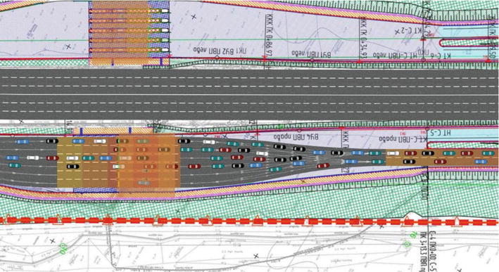
Consider the WHSD interchange at the intersection with Shuvalovsky Ave. This interchange is also located in the Primorsky District of St. Petersburg, a large part of which is included in the interchange gravity zone.

The Shuvalovsky interchange allows to relieve the traffic load both from the street and road network of the district and from the TP at the exit from the WHSD to Bogatyrsky Ave., which was assessed by the authors earlier in Section 3 as well as in the articles [33, 39].

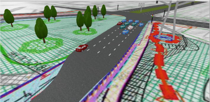
The exit from the toll road is a TP consisting of six toll lanes, with four lanes operating in automatic mode and two lanes in manual mode combined with ETC payment mode. A general view of the TP at the Shuvalovsky Ave. exit is shown in Figure 14.

Figure 14.

General view of the TP at the Shuvalovsky Ave.

The connection of the toll road exit to the street and road network of the district is via a controlled intersection located 475 meters behind the TP and providing exits for traffic on Shuvalovsky Ave. and Planernaya St. The connection to the controlled intersection is in four traffic lanes, three of which prescribe forward traffic on Shuvalovsky Ave. and one providing a right turn onto Planernaya St.

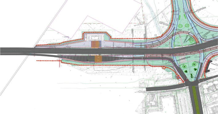
The general view of the toll road exit connection to the regulated intersection is shown in Figure 15.

Figure 15.

General view of the toll road exit connection to the regulated intersection.

A special feature of this exit is the so-called bottlenecks before the TP and the controlled intersection—two-lane sections of road at the exit from the main course of the road before the entrance area to the TP and a two-lane section of road at the exit from the TP before the approach area to the traffic light facility. This feature allows the road section to be considered as a sequence of “obstacles” slowing down traffic speeds and affecting its capacity.

The main traffic correspondences of the area are home-work and work-home. The congestion on the outbound TP located on Shuvalovsky Ave. usually occurs during evening rush hours. A SM has been developed to assess the traffic conditions in the interchange area. The model study area starts from the WHSD exit and ends with the exit to Shuvalovsky Ave. and Planernaya St. behind the regulated intersection and includes the TP and the traffic light facility, the current operation modes of the TP and traffic lights are reproduced. The general view of the SM of the interchange is shown in Figure 16.

Figure 16.

The general view of the SM of the interchange at the intersection with Shuvalovsky Ave.

The distribution of manual and automatic toll lane service times is defined in the SM parameters.

The general view of the developed SM of the TP at Shuvalovsky Ave. is shown in Figure 17.

Figure 17.

The general view of SM of the TP at Shuvalovsky Ave.

The SM of the controlled intersection is aimed at evaluating the efficiency of the traffic light phasing that ensures the exit of the vehicles from the interchange area. Thus, this traffic light facility reproduces the regulation of correspondence in the directions of traffic “TP-Shuvalovsky” and “TP-Planernaya St.”. It should be noted that these directions are regulated separately as the right turn from the right lane is regulated by an additional traffic light section. The actual duration of the traffic light phases is shown in Table 9.

Traffic light phase	Straight ahead (Shuvalovsky Ave.), sec.	Turn right (Planernaya Str.), sec.
Red	80	56
Yellow	3	—
Green	32	58
Yellow	4	—

Table 9.

Actual duration of traffic light phases after exiting the toll road.

A general view of the SM of the toll road exit connection to a controlled intersection is shown in Figure 18.

Figure 18.

General view of the SM of the toll road exit connection to a controlled intersection.

The sequential location of the TP and the traffic light facility can lead to the following traffic situations:

1. In case of insufficient capacity of the TP and a high volume of traffic passing through the crossing point, traffic congestion can occur in front of the TP;

2. If there is insufficient operating time for traffic lights providing an exit from the TP, there can be a risk of congestion in front of the intersection. Since the regulated intersection is 475 meters from the toll road, if the length of congestion exceeds this distance, there may be an additional risk of increased service time for users at the exit of the toll road.

With the help of the traffic interchange developed by the SM, the following were carried out:

1. Analysis of the capacity of the TP at the exit of the toll road;

2. Analysis of traffic capacity of traffic interchange, including functioning TP and controlled traffic light object;

3. Evaluation of the possibility of optimizing the operation of the traffic light facility to increase the capacity of the interchange.

5.2 Assessing the capacity of the toll plaza

The capacity limit is the capacity at which, when passing through the toll lanes, the vehicles queued beyond the approach area of the TP—the line beyond which the widening of the road section from two to six lanes begins. The operation of the traffic light behind the checkpoint was not considered to assess the capacity of the TP.

In this study, traffic flow parameters were selected, advising data for the year 2021. For example, the proportion of traffic flow users using ETC devices to pay at an automated lane is 93%. In this location, the assumption of homogeneity of the traffic flow consisting of passenger cars is acceptable, as there are practically no heavy vehicles at the studied interchange.

A number of simulations were carried out with traffic intensity ranging from 100 to 4000 vehicles/h in steps of 50 vehicles/h in order to estimate the maximum load on the TP. A study of the operation of the TP at different traffic intensities revealed that at low intensities the service time distribution was a mixture of split distribution laws, corresponding to the passage of vehicles through manual and automatic toll lanes.

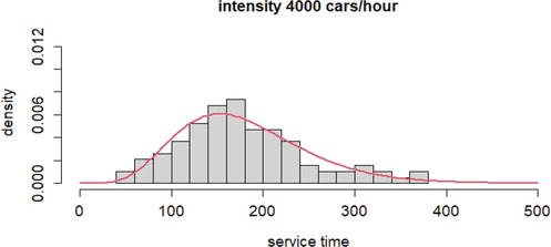
At high intensities with vehicle queues forming outside the approach area to the TP, the distribution of time spent in automatic and manual toll lanes formed an undivided mixture of distributions that approximates well to the gamma distribution law. The distribution of service times at the TP with 4000 vehicles/h is shown in Figure 19. This distribution has a strong right-hand asymmetry. An indirect characteristic of this asymmetry is the significant difference between the mean and the most likely passing time at the TP.

Figure 19.

The distribution of service times at the TP with 4000 vehicles/h.

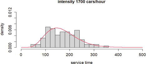
As a result of the simulation experiments, it was found that the throughput capacity of the developed SM of the TP at the set traffic flow parameters corresponds to a capacity of 1700 vehicles/h. The distribution of the service time at the TP at 1700 vehicles/h is shown in Figure 20.

Figure 20.

The distribution of the service time at the TP at 1700 vehicles/h.

5.3 Interchange capacity analysis

In order to analyze the traffic capacity of the interchange, simulation experiments were carried out to investigate the traffic flow time through the TP and the controlled intersection under actual parameters of the phase duration of the traffic light providing the exit from the TP.

A number of simulation experiments were conducted with traffic volumes ranging from 100 to 4000 vehicles/h in increments of 50 vehicles/h.

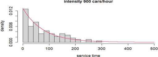
As a result of these simulations, it was found that with the existing traffic light phasing parameters, traffic congestion begins to form in front of the intersection when the intensity exceeds a value of more than 900 vehicles/h. When the queue of vehicles exceeds a distance of more than 475 meters, congestion occurs in the exit area of the TP, resulting in reduced service times in the toll lanes and the appearance of a second congestion before entering the TP area. An example of traffic congestion in the TP exit area is shown in Figure 21. The distribution of service times at the TP with a traffic volume of 900 vehicles/h is shown in Figure 21.

Figure 21.

Traffic congestion in the TP exit area at the intraurban toll road exit to the urban street and road network.

At an inbound traffic intensity of 900 vehicles/h, there is no longer a separable mixture of vehicle travel time distributions through the TP zone, but the observed empirical distribution (Figure 22) is well approximated by an exponential law (a particular case of a gamma distribution).

Figure 22.

Distribution of service times at the TP with an input flow rate of 900 vehicles/h.

5.4 Interchange capacity optimization

Let us consider the process of accumulation of vehicles on the road section from the exit from the TP zone to the traffic light facility (its length is 475 meters, and the maximum capacity is about 160 vehicles, at the rate of 8 meters per 1 vehicle, two-thirds of the section are two lanes, one-third of the section is four lanes). Let the inbound flow of vehicles be modeled by the Poisson flow of vehicles with intensity $\lambda$ (the moment of vehicle arrival is considered to be the moment when the front bumper of the vehicle crosses the end line of the TP zone). Within one cycle of the traffic light object, we will consider this intensity as constant. The moment when the vehicle leaves the whole junction zone, we will consider crossing by the rear bumper of the vehicle of the line on which the traffic light is installed. At opening of a green light, the first vehicles in lanes (if they are there) start moving increasing speed from zero value. The following vehicles cross the end line of the junction area at a higher speed. Consequently, when crossing the traffic light line, there is a flow with variable intensity $\mu \left(t\right)$ within the green (and yellow) phase of the traffic light from 0 to $\tau$. Let the full cycle of the traffic light object is T, the duration of the green and yellow phases is $\tau$, and the red phase is T−$\tau$. Let $X$ be a random variable, let the full cycle of the traffic light object is T, and the duration of the green and yellow phases is $\mathit{\lambda T}$, that is

$$P\left(X=m\right)=\frac{{\mathit{\lambda T}}^m}{m!}{e}^{-\mathit{\lambda T}}$$E26

Let $Y$ be a random variable, the number of vehicles leaving the interchange area (crossing the traffic light line) for time $\tau$, distributed according to Poisson distribution with changing parameter $\mu \left(t\right)$. Then, the accumulated intensity of the vehicles leaving the interchange area ${\rm M}\left(0,\tau \right)=\underset{0}{\overset{\tau }{\int }}\mu \left(t\right)\mathit{dt}$. In the remaining time interval T−$\tau$ the intensity of the vehicle leaving the decoupling zone is equal to zero. The difference $Z=X-Y$ is the number of vehicles remaining on the section (arriving but not having time to leave it during one cycle of the traffic light object). The random variable Z, as the difference between two Poisson random variables, has Skellam’s distribution law [34]:

$$f\left(k,\mathit{\lambda T},\underset{0}{\overset{\tau }{\int }}\mu \left(t\right)\mathit{dt}\right)=P\left(V=k\right)=e^{-\left(\mathit{\lambda T}+\underset{0}{\overset{\tau }{\int }}\mu \left(t\right)\mathit{dt}\right)}{\left(\frac{\mathit{\lambda T}}{\underset{0}{\overset{\tau }{\int }}\mu \left(t\right)\mathit{dt}}\right)}^{\frac{k}{2}}{I}_{\left|k\right|}\left(2\sqrt{\mathit{\lambda T}\times \underset{0}{\overset{\tau }{\int }}\mu \left(t\right)\mathit{dt}}\right).$$E27

where $I_{\left|k\right|}\left(x\right)$ is a modified Bessel function of the first kind, with $k=0,\pm 1,\pm 2,\dots ,\pm \infty$.

In reality, the value of Z cannot take negative values. Therefore, the distribution function of a random variable Z can be written as

$$\left\{\begin{array}{c}P\left(Z=0\right)=e^{-\left(\mathit{\lambda T}+\underset{0}{\overset{\tau }{\int }}\mu \left(t\right)\mathit{dt}\right)}\sum _{k=0}^{-\infty }{\left(\frac{\mathit{\lambda T}}{\underset{0}{\overset{\tau }{\int }}\mu \left(t\right)\mathit{dt}}\right)}^{\frac{k}{2}}{I}_{\mid k\mid }\left(2\sqrt{\mathit{\lambda T}\underset{0}{\overset{\tau }{\int }}\mu \left(t\right)\mathit{dt}}\right),\mathit{at}k\le 0,k\in Z\\ P\left(V^{\ast }=k\right)=e^{-\left(\mathit{\lambda T}+\underset{0}{\overset{\tau }{\int }}\mu \left(t\right)\mathit{dt}\right)}{\left(\frac{\mathit{\lambda T}}{\underset{0}{\overset{\tau }{\int }}\mu \left(t\right)\mathit{dt}}\right)}^{\frac{k}{2}}{I}_k\left(2\sqrt{\mathit{\lambda T}\underset{0}{\overset{\tau }{\int }}\mu \left(t\right)\mathit{dt}}\right),\mathit{at}k>0,k\in Z\end{array}\right.$$E28

During traffic simulation experiments in the junction area, the exit from the WHSD to Shuvalovsky Ave. with the parameters of the TP and the traffic light facility, it was found that traffic congestion on the section between the TP exit and the traffic light line is consistently formed at an input flow rate of 900 vehicles/h, which amounts to 30 vehicles per 2 minutes. The TP is able to pass up to 1700 vehicles/h without jamming. Thus, the congestion is caused as a consequence of the sub-optimal operation of the traffic light. The task is to determine an optimal traffic light solution that allows passage of up to 1700 vehicles/h without jamming on the section between the TP exit and the traffic light.

The integrated OptQest optimizer in AnyLogic was used to find an appropriate solution. The optimization result is presented in Table 10.

Parameters		Current	Best
Direction	Traffic light phase
Straight	Green	49	120
Straight	Red	66	40
Right turn	Green	95	16
Right turn	Red	72	13

Table 10.

The best settings for traffic light phases at the exit from the TP.

After the optimization of the traffic light phases at the TP exit, a number of simulations were carried out to assess the traffic capacity of the interchange. The results of the simulations showed that when the traffic light phases specified in Table 10 are set, the capacity of the whole interchange coincides with the throughput capacity of the TP—1700 vehicles/h.

At any traffic intensity exceeding the value of 1700 vehicles/h, there is no congestion in front of the controlled intersection, because the traffic light phases are set so that the outgoing flow in a sufficiently long time corresponds to the traffic intensity of 1700 vehicles/h—the maximum intensity of the flow coming from the TP area. In this case, congestion will only occur in front of the TP.

6. Conclusion

Using the example of the WHSD toll road, the SMs of the different types of intraurban toll roads are constructed:

1. Toll road exit TP;

2. TP on the main course of a toll road;

3. TP at the exit from the toll road before the controlled intersection.

The SMs have both the parameters of the general simulation methodology and additional parameters affecting the intensity. As a result of the experiments, the traffic intensities at the TPs at which congestion starts to form were determined.

For each of the cases considered, the parameters of the gamma-law distribution of service times were determined. The results of the study show that when there is insufficient capacity, the TP ceases to operate efficiently and the user service time increases, regardless of the fare type.

The methods and SMs described above can be used in estimating the existing and projected capacity of the TPs in operation. With capacity data and model parameters obtained under toll road operating conditions, the toll road operator can more accurately evaluate the parameters for optimizing or upgrading the tolling system as well as other measures to increase TP capacity.

The described methodology is applicable to intraurban toll roads located in a balanced residential area with a high volume of pendulum migration. Also note that when the TPs are located in pronounced industrial-logistic areas of the city, as well as in the border areas between the city and the region, the analysis of TPs capacity may require additional assessment of traffic intensity under different conditions, taking into account daily, weekly and seasonal and irregular flow patterns.

Acknowledgments

The research was carried out at the expense of the Russian Science Foundation grant No 20-18-00365, https://rscf.ru/project/23-18-45035/