Investigation on the Performance Efficiency of the Shunt Hybrid Active Power Filter

Abstract

The disturbances observed in the electrical system such as harmonics, asymmetry, flickers, voltage dips and swells, transients, are due to the type of connected devices. The nonlinear devices are the most common ones. Their connection to the electrical system without solution of mitigating their negative influence on supply network can be the cause of poor power quality. There are different types of solutions such as the passive harmonic filters (PHF), the active power filters (APF), the hybrid active power filters (HAPF). Each of those solutions presents some advantages and disadvantages. The chapter is focused on the HAPF, which is the combination of the PHF and shunt active power filter (SAPF) connected in series. Such topology is known in the literature, but still, there are certain problems that need more clarification through detailed studies. For instance, there are not enough recommendations on how to choose the PHF tuning frequency, when it is connected in series with SAPF. The investigations presented in this chapter are very detailed and based on a case study. The proposed control system algorithms of filters (SAPF and HAPF) are presented as well as formulated recommendations.

1. Introduction

In today societies, the production of nonlinear loads such as household appliances and industries electrical devices is in full grow. Their mass connection to the supply network (despite their compliance with standards) may cause a deterioration of the power quality.

The power quality refers mostly to the supply voltage quality (frequency, amplitude, waveform, unbalance, etc.) which should be in accordance with the recommendations set by the national or international standards (e.g., EN 50160 [1]).

If the supply voltage at the point of common coupling (PCC) presents poor quality (not complying standards), its improvement is therefore necessary. The poor power quality does not come from the energy producer (because the voltage at the terminal of power plants is almost without disturbances), but mainly from connected disturbing devices such as power electronic devices (e.g., diode and thyristor bridges), arc devices (e.g., arc furnaces, welding devices, discharge lamps), saturated magnetic cores devices (e.g., transformers, motors).

The electrical power is as a commodity and taking care of its quality is necessary. The power quality disturbances are numerous and varied (e.g., voltage drops and swells, flickers, harmonics, asymmetry) and their presence in the electrical system has consequences on the connected devices. For instance, the harmonics, if not mitigated can cause the increase of current RMS value; the overloading, overheating, and even damage of power system elements (e.g., transformers, generators, cables, electric motors, capacitors) and other connected devices (e.g., household appliances); the reduction of devices life span; the perturbation of the devices normal operation and power system operating costs increase; the inaccurate measurements of energy and power; decrease of power factor (PF), etc. [2, 3, 4].

To maintain the grid power quality in compliance with the standards, many solutions are proposed, including passive harmonic filters (PHF), active power filter (APF), hybrid power harmonic filter (HPHF), etc. [5]. Each of the solution presents advantages and disadvantages. The PHFs are applied in most cases for harmonics filtration and fundamental reactive power mitigation [6]. They present disadvantages such as: fixed reactive power and fixed tuning frequencies (e.g., designed for a defined load parameters), grid parameter dependency (e.g., grid impedance of the harmonic to be eliminated), resonance (series and parallel) problem, sensitive to the tolerance of its elements (e.g., reactor inductance), detuning phenomenon because of the aging, power losses in the case of filters with damping resistance (e.g., broad-band PHFs). Despite their drawbacks, the PHFs are still applied in practice and from the economical point of view, they are more preferred than the shunt active power filters (SAPFs) [7, 8, 9, 10].

In comparison with the PHFs, the SAPFs are more efficient and their application is growing in low and medium voltage systems, particularly in the industries [11, 12]. The goal of their application can be the mitigation of disturbances such as current/voltage harmonics, asymmetry, and reactive power compensation (fundamental component). Their disadvantages are high cost [13], complex control system, difficulty for large-scale implementation [14, 15].

The hybrid filter topologies are diversified in the literature [16]. They result from the combination of the shunt or series APF with the parallel PHF or the shunt APF with the series APF. The main advantages of combining the active and passive filters together are as follows: (a) The power demand and performance cost of the active part are less than when it is operating alone and (b) the overcoming of the passive part disadvantages (e.g., resonance phenomena, grid impedance dependency) [17, 18].

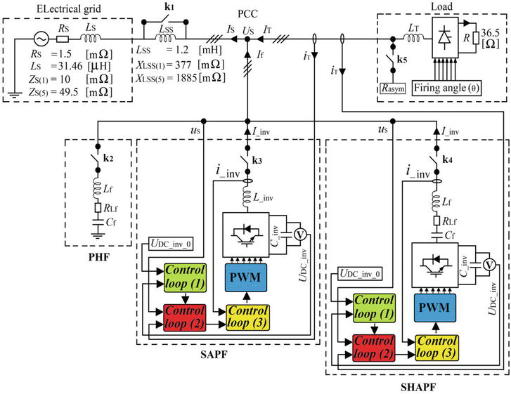
The shunt hybrid active power filter (SHAPF) under study in the chapter is a structure known in the literature. It is composed of PHF connected in series with the SAPF (Figure 1) [19, 20]. The SAPF when operating alone is always connected to the full-supply phase-to-phase PCC voltage and need for its proper operation, a high rate of inverter DC voltage (e.g., 710 V and more [21, 22]). But connected in series with the PHF, the passive part allows the active part to work under a small rate of inverter voltage, therefore reducing its initial and operating cost [23, 24, 25, 26]. The investigated SHAPF is for the grid current harmonics and fundamental harmonic reactive power compensation and its DC voltage is fixed at 150 V and can be less (e.g., 70 V (see [27])).

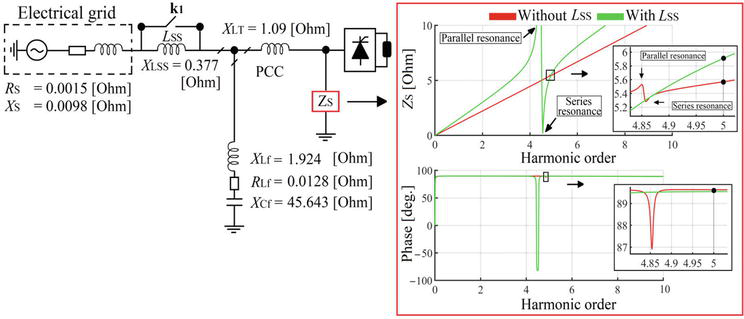
Figure 1.

Electrical system together with the investigated filters (k1-k5—Switches).

In the literature, there are not many clarifications on how to choose the tuning frequency of the PHF when it is connected in series with the inverter (SAPF). In Refs. [28, 29, 30] for instance, it is recommended to tune it to the 7th harmonic frequency because it is then less bulk, low cost and presents lower impedance for the 11th and 13th harmonic frequencies than in the case when it is tuned to the 5th harmonic frequency. It is difficult to find papers presenting the investigations in which the SHAPF work efficiency is compared after tuning the passive part to different frequency. In this chapter, such investigations are proposed.

The chapter is organized in five parts: The first one presents the electrical system (grid and load) in which the analyses are performed; the second part presents the influence of the grid parameters on the PHF performance efficiency. In the third part, the SAPF with input reactor is investigated. In fourth one, the SHAPF with proposed control system is considered. The last part contains the conclusion. All the chapter investigations are performed in MATLAB/SIMULINK [31].

2. Electrical system description

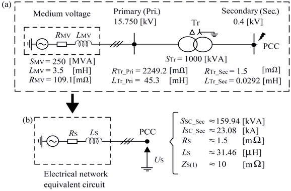
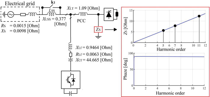
The electrical system environment in which the filters are investigated is presented in Figures 1 and 2. The electrical grid equivalent parameters in Figure 2 are taken from the laboratory setup.

Figure 2.

(a) Parameters of the electrical grid taken from the laboratory set up, (b) electrical grid equivalent circuit.

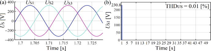
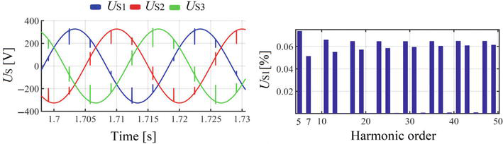
In Figure 3(a) and (b), it can be seen the PCC voltage waveforms together with the spectrum when the filters and load are not connected. The load is presented in Figure 1. It constitutes of six-pulse thyristor bridge with resistance (R) at DC side and input reactor ($L_{\mathrm{T}}$). The phase-to-phase connected resistance $R_{\text{asym}}$ (k5 closed) is used to create load asymmetry in the electrical system in the investigation frame of the SAPF and SHAPF.

Figure 3.

(a) PCC voltage waveforms without any load or filter connected with (b) the spectrum (one-phase representation because of the symmetrical system).

The additional line reactor $L_{\mathrm{SS}}$ (see Figure 1) connected between the grid and the PCC will be used in the investigations case of the PHF. Other parameters (e.g. L_T, filters) of the electrical system in Figure 1 will be presented later.

3. Investigation on the grid dependency of the PHF work efficiency

This chapter investigates and compares two case studies: In the first one, the PHF is connected to the electrical system where the grid equivalent impedance for the harmonic to be eliminated ($Z_{\mathrm{S}\left(5\right)}$) is smaller than the one of the filter ($Z_{\mathrm{f}\left(5\right)}$). In the second one, the PHF is connected to the electrical system where the grid equivalent impedance for the harmonic to be eliminated ($Z_{\mathrm{S}\left(5\right)}$) is increased by the additional line rector ($L_{\mathrm{SS}}$) and is therefore higher than the one of the filter ($Z_{\mathrm{f}\left(5\right)}$).

3.1 Simulation assumptions

The simulations are performed based on the assumptions that: the supply voltage before the PHF and the load connection does not contain harmonic (see Figure 3), the resistance of the additional line reactor ($L_{\mathrm{SS}}$) as well as the one of the thyristor bridge input reactor ($L_{\mathrm{T}}$) are neglected, the switches k3, k4, and k5 are opened and k2 is close (Figure 1). The switch k1 will be opened and closed depending on the case study. The electrical grid equivalent impedance for the 5th harmonic ($Z_{\mathrm{S}\left(5\right)}$—Figure 1) is computed considering the electrical system parameters from the medium voltage side of the transformer (see Figure 2(a)). The 5th harmonic is the lowest characteristic harmonic generated by the load (after the fundamental) according to the formula $6k\pm 1$ wehre $k>0$. Because of the symmetrical system, the results are presented only for one-phase.

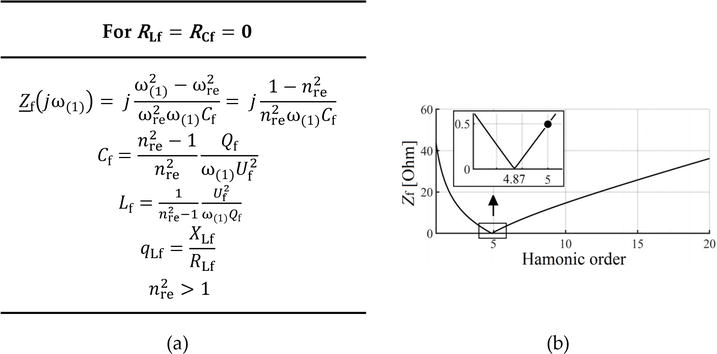
3.2 Design of the PHF

The formula used to compute the PHF parameters is presented in Figure 4(a) and its impedance versus frequency characteristic is shown in Figure 4(b). Because of the aging, the PHF is tuned to the frequency of 243.5 Hz ($n_{\mathrm{re}}=4.87$) which is a bit lower than the frequency of harmonic to be eliminated (5th). The computed parameters are shown in Table 1. Comparing the 5th harmonic equivalent impedance of the PHF ($Z_{\mathrm{f}\left(5\right)}=490\left[\mathrm{m\Omega }\right]$) to the one of the grid ($Z_{\mathrm{S}\left(5\right)}=49.5\left[\mathrm{m\Omega }\right]$, when $L_{\mathrm{SS}}$ is not considered). It can be notices that (see Table 1) the one of the PHF is almost 10 times higher than the one of the grid, which allows to conclude that a big part of the 5th harmonic current coming from the load will not be filtered. That situation is contrary when the addition line reactor $L_{\mathrm{SS}}$ is considered ($Z_{\mathrm{S}\left(5\right)}=1934\left[\mathrm{m\Omega }\right]$ is almost 4 times higher than $Z_{\mathrm{f}\left(5\right)}$).

Figure 4.

(a) Expressions used to compute PHF parameters ($q_{\mathrm{Lf}}$—Reactor quality factor, $n_{\mathrm{re}}$—order of the resonance frequency), (b) PHF impedance versus frequency characteristic.

$n_{\mathrm{re}}$	$Q_{\mathrm{f}}$; [Var]	$U_{\mathrm{f}}$; [V]	$L_{\mathrm{f}}$; [mH]	$C_{\mathrm{fY}}$ [μF]	$q_{\mathrm{Lf}}$	$Z_{\mathrm{f}\left(1\right)}$ [Ω]	$Z_{\mathrm{f}\left(5\right)}$ [Ω]	$L_{\mathrm{SS}}$; [mH]	$Z_{\mathrm{S}\left(5\right)}$[Ω]; (without $L_{\mathrm{SS}}$)	$Z_{\mathrm{S}\left(5\right)}$[Ω]; (with $L_{\mathrm{SS}}$)
4.87	1210	230	6.1	69.73	150	43.71	0.49	1.2	0.0495	1.934

Table 1.

Computed equivalent parameters of the PHF (one-phase).

3.3 Simulation results

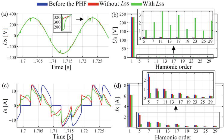
The simulation data before the PHF connection, with and without the grid side line reactor $L_{\mathrm{SS}}$ are compared based on: grid voltage and current waveforms, characteristic harmonics (Figure 5), THD, grid, and filter active and reactive powers (fundamental harmonic, Figure 6) as well as the electrical system impedance versus frequency characteristics seen from the thyristor bridge input (Figure 7).

Figure 5.

(a) Grid voltage/current waveforms and their (b) spectrums (the red and green colors represent the cases when the filter is connected).

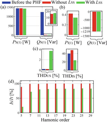
Figure 6.

(a) Grid active ($P_{\mathrm{S}\left(1\right)}$) and reactive power ($Q_{\mathrm{S}\left(1\right)}$), (b) filter active ($P_{\mathrm{f}\left(1\right)}$) and reactive ($Q_{\mathrm{f}\left(1\right)}$) power, (c) grid voltage and current THD, and (d) PHF work efficiency on harmonics reduction (the red and green colors represent the cases when the filter is connected).

Figure 7.

Impedance versus frequency characteristics of the electrical system seen from the thyristor bridge input terminals.

Figure 5(a) represents the grid voltage waveforms and Figure 5(b) its spectrum (for the current—Figure 5(c) and (d), respectively). It can be noticed that when the additional line reactor $L_{\mathrm{SS}}$ is connected (k1 open), all the harmonics amplitudes of the grid voltage have increased (Figure 5(b)), whereas the ones of the grid current have decreased (Figure 5(d)). The 5th harmonic current amplitude is therefore better reduced at the grid side (Figure 5(d)).

In Figure 6(a), the grid active powers ($P_{\mathrm{S}\left(1\right)}$) are almost the same and it can also be seen that after the PHF connection, in both cases (without and with $L_{\mathrm{SS}}$) the grid reactive powers are well reduced but the reduction is a bit better in the case without $L_{\mathrm{SS}}$.

With the additional line reactor, the PHF presents less power losses (Figure 6(b)); the grid voltage is more distorted (Figure 6(c)) and the grid current is less distorted (see THD in Figure 6(c)). The increase of the grid current total harmonic distortion (${\mathrm{THD}}_{\text{IS}}$—Figure 6(c)) after the PHF connection (case without $L_{\mathrm{SS}}$) is due to fact that the grid current fundament harmonic amplitude has decreased because of the reactive power compensation and the harmonics have almost not been reduced (1).

$${\mathrm{THD}}_{\mathrm{I}}=\frac{\sqrt{{\sum }_{k=2}^{50}{I}_k^2}}{I_1}$$E1

Figure 6(d) presents the PHF work efficiency in terms of harmonics reduction. It represents the percentage of current harmonics flowing from the load to the grid after the PHF connection (without and with L_SS). It can be observed that without L_SS in the electrical system, almost 100% of current harmonics generated by the load flow to the grid. The connection of $L_{\mathrm{SS}}$ has improved the PHF work efficiency especially on the 5th harmonic reduction (Figure 6(d)).

The impedance versus frequency characteristics of the electrical system seen from the thyristor bridge input are presented in Figure 7. It can be observed in the both cases (without and with $L_{\mathrm{SS}}$), the parallel and series resonances. The series resonance comes from the PHF and the parallel resonance comes from the parallel connection between the grid and the PHF. The resonances are below the 5th harmonic, which means that the filter was well deigned. Such harmonics (at the resonance) do not exist in considered system.

The performed studies have clearly showed that the PHF work efficiency in terms of harmonics mitigation strongly depends on the electrical grid parameters. Because of that it is necessary to obtain the information about the grid equivalent impedance for the harmonic to be eliminated (through the electrical system short-circuit power at the PCC) before the filter installation. In the case where that equivalent impedance is smaller than the one of the PHF, the solution can be the use of an additional line reactor between the PCC and the grid to increase the filtration effectiveness as it has been demonstrated in the chapter.

4. Investigation on the influence of the thyristor bridge input reactor size on the SAPF work efficiency

The work efficiency of the SAPF does not depend only on the designed control system or inverter parameters, but also on the parameters of the electrical system to which it is connected. For instance, in the electrical system with a diode or thyristor bridge as load, the accepted operating efficiency of the SAPF (with input reactor as switching ripple filter) may not be met due to the high rate of load current change (di/dt) at the points of commutation notches. Therefore, it is necessary to study and know the electrical system (grid and load sides) before its installation. That problem is also mentioned in the literature [21]. In this chapter, it is demonstrated that to obtain a better SAPF work efficiency, its input reactor parameters (see $L_{\_\mathrm{inv}}$ in Figure 1) should be selected based not only on the effective reduction of the inverter switching ripple or the control system demand, but also on the load parameters, such as the parameters of the diode or thyristor bridge input line reactor (see $L_{\mathrm{T}}$ in Figure 1). For a good clarification, two case studies are considered in the chapter: In the first one, it is presented the influence of the SAPF input reactor size (load input reactor constant) on its work efficiency. In the second one, it is presented the influence of the load input reactor on the SAPF work efficiency (SAPF input reactor constant).

4.1 Simulation assumptions

The SAPF control system and DC capacitor ($C_{\_\mathrm{inv}}$) parameters are constant, the load input reactor resistance as well as the one at the SAPF input is neglected, the additional line reactor L_SS is not considered (k1 closed), the asymmetry resistance ($R_{\text{asym}}=60\mathrm{\Omega }$) is considered (k5 closed), the load DC resistance is constant, the switches k2 and k4 are opened, and k3 is closed. The SAPF switching frequency is fixed to 20 kHz.

4.2 Description of the SAPF as well as its control system

The SAPF presented in Figure 1 is three legs three wires invert with an reactor ($L_{\_\mathrm{inv}}$) at its input and capacitor ($C_{\_\mathrm{inv}}$) at its DC side. Its proposed control system is presented in Figure 8 and is organized in three control loops: (1)–(3).

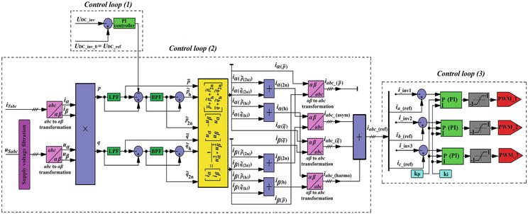
Figure 8.

Block diagram of the SAPF control system: a, b, and c—Phase designations of the supply network; 1, 2, and 3—represent the inverter inputs.

The role of the control loop (1) is to maintain the SAPF DC voltage ($U_{\mathrm{DC}\_\mathrm{inv}}$) constant and at the level as the given reference voltage ($U_{\mathrm{DC}\_\mathrm{ref}}$) [32].

The control loop (2) algorithm is based on the time domain instantaneous p-q theory [33]. Its role is to split the distorted instantaneous load current ($i_{\mathit{\text{Tabc}}}$) into four different components related to (see Figure 8): active ($i_{\mathit{abc}\_\left(\overline{p}\right)}$), reactive ($i_{\mathit{abc}\_\left(\overline{q}\right)}$), asymmetry ($i_{\mathit{abc}\_\left(\text{asym}\right)}$), and harmonic ($i_{\mathit{abc}\_\left(\mathit{\text{harmo}}\right)}$). The output signal of the control loop (2) is therefore the instantaneous reference current ($i_{\mathit{abc}\_\left(\mathrm{ref}\right)}$) which is constituted of three components (reactive, asymmetry, and harmonic currents) as shown in Figure 8 (the active component ($i_{\mathit{abc}\_\left(\overline{p}\right)}$) is not included).

Observing the control loop (2) algorithm, it can be noticed that the splitting of the instantaneous load current ($i_{\mathit{\text{Tabc}}}$) into different components starts from its measurement as well as the measurement of the instantaneous PCC voltage ($u_{\mathit{\text{Sabc}}}$). The supply voltage is filtered (“supply voltage filtration”) to avoid its distortions to be found on the reference courant. The instantaneous real (p) and imaginary (q) powers are obtained after transforming the instantaneous PCC voltage and current from the a-b-c coordinates to the α-β rectangular coordinates. The low-pass filter (LPF) and band-pass filter (BPF) are used to filter the instantaneous real (p) and imaginary (q) powers so that their components (($\overline{p}$, $\overline{q}$)—constant components related to the fundamental harmonic (positive sequence), (${\stackrel{\sim }{p}}_{\mathrm{h}}$, ${\stackrel{\sim }{q}}_{\mathrm{h}}$)—component related to the current harmonic and (${\stackrel{\sim }{p}}_{2\mathrm{n}}$, ${\stackrel{\sim }{q}}_{2\mathrm{n}}$)—component related to the current asymmetry (negative sequence of the fundamental harmonic)) can be used in the matrix (see Figure 8) to compute the instantaneous currents ($i_{\alpha },i_{\beta }$) in α-β axes. After the matrix computation, different current components are obtained: ($i_{\mathrm{\alpha }\left(\overline{\mathrm{p}}\right)},i_{\mathrm{\beta }\left(\overline{\mathrm{p}}\right)})$—instantaneous real current (fundamental harmonic) in α and β axes respectively, (($i_{\mathrm{\alpha }\left({\stackrel{\sim }{\mathrm{p}}}_{2\mathrm{n}}\right)},i_{\mathrm{\alpha }\left({\stackrel{\sim }{\mathrm{q}}}_{2\mathrm{n}}\right)}$), ($i_{\mathrm{\beta }\left({\stackrel{\sim }{\mathrm{p}}}_{2\mathrm{n}}\right)},i_{\mathrm{\beta }\left({\stackrel{\sim }{\mathrm{q}}}_{2\mathrm{n}}\right)}$))—instantaneous asymmetry current in α and β axes, respectively, (($i_{\mathrm{\alpha }\left({\stackrel{\sim }{\mathrm{p}}}_{\mathrm{h}}\right)},i_{\mathrm{\alpha }\left({\stackrel{\sim }{\mathrm{q}}}_{\mathrm{h}}\right)}$), ($i_{\mathrm{\beta }\left({\stackrel{\sim }{\mathrm{p}}}_{\mathrm{h}}\right)},i_{\mathrm{\beta }\left({\stackrel{\sim }{\mathrm{q}}}_{\mathrm{h}}\right)}$))—instantaneous harmonic current in α and β axes respectively, ($i_{\mathrm{\alpha }\left(\overline{\mathrm{q}}\right)},i_{\mathrm{\beta }\left(\overline{\mathrm{q}}\right)})$—instantaneous imaginary current (fundamental harmonic) in α and β axes respectively. The components such as $i_{\alpha \left(2\mathrm{n}\right)}$ and $i_{\beta \left(2\mathrm{n}\right)}$ are the instantaneous asymmetry current in α and β axis respectively and the components such as $i_{\alpha \left(\mathrm{h}\right)}$ and $i_{\beta \left(\mathrm{h}\right)}$ are the instantaneous harmonics current in α and β axis respectively.

In the control loop (3), the instantaneous reference current ($i_{\mathrm{abc}\_\left(\mathrm{ref}\right)}$) is compared to the feedback loop current coming from the inverter input ($i_{\_\mathrm{inv}123}$). It can also be seen the blocks of PI controller, saturation, and pulse-width modulation (PWM) system.

4.2.1 Computation of the SAPF parameters

The proposed expressions used to compute the SAPF parameters are presented in (2)-(4) and the computed parameters in Table 2. The PI controller parameters are presented in Table 3.

$∆U_{\mathrm{L}\_\mathrm{inv}}$; [V]	$L_{\_\mathrm{inv}\_min}$; [mH]	$L_{\_\mathrm{inv}\_max}$; [mH]	$I_{a\_\left(\mathrm{ref}\right)}$; [A]	$I_{b\_\left(\mathrm{ref}\right)}$; [A]	$I_{c\_\left(\mathrm{ref}\right)}$; [A]	${\mathrm{k}}_{\mathrm{DC}}$	$U_{\mathrm{S}\_\mathrm{p}-\mathrm{p}}$; [V]	$U_{\mathrm{DC}\_\mathrm{inv}\_0}$; [V]	$∆W_{\mathrm{DC}\_\mathrm{inv}}$; [J]	$∆U_{\mathrm{DC}\_\mathrm{inv}}$; [V]	$C_{\_\mathrm{inv}}$; [mF]
3	1.4	—	4.46	9.38	7.34	1.32	400	750	11	5	3
16	—	7.2

Table 2.

Computed SAPF parameters.

	kp	ki
Control loop (1)	40,000	43.75
Control loop (3)	250	0.0001

Table 3.

PI controller parameters.

$${\mathit{U}}_{\mathrm{DC}\_\mathrm{inv}\_0}\mathbf{>}{\mathbf{k}}_{\mathrm{DC}}\left(\sqrt{\mathbf{2}}{\mathit{U}}_{\mathrm{S}\_\mathrm{p}-\mathrm{p}}\right),{\mathbf{k}}_{\mathrm{DC}}\mathbf{>}\mathbf{1}$$E2

$${\mathit{L}}_{\_\mathrm{inv}}\mathbf{=}\frac{\mathbf{3}\mathbf{∆}{\mathit{U}}_{\mathrm{L}\_\mathrm{inv}}}{{\mathbf{\omega }}_{\left(\mathbf{1}\right)}\left({\mathit{I}}_{\mathit{a}\_\left(\mathrm{ref}\right)}\mathbf{+}{\mathit{I}}_{\mathit{b}\_\left(\mathrm{ref}\right)}\mathbf{+}{\mathit{I}}_{\mathit{c}\_\left(\mathrm{ref}\right)}\right)}$$E3

$${\mathit{C}}_{\_\mathrm{inv}}\mathbf{=}\frac{\mathbf{∆}{\mathit{W}}_{\mathrm{DC}\_\mathrm{inv}}}{{\mathit{U}}_{\mathrm{DC}\_\mathrm{inv}\_0}\mathbf{∆}{\mathit{U}}_{\mathrm{DC}\_\mathrm{inv}}}$$E4

Where: ${\mathit{U}}_{\mathsf{S}\_\mathsf{p}-\mathsf{p}}$—phase-to-phase PCC voltage, ${\mathbf{k}}_{\mathsf{DC}}$—coefficient, $\mathbf{∆}{\mathit{U}}_{\mathsf{L}\_\mathsf{inv}}$—inverter input reactor voltage drops, ${\mathit{I}}_{\mathit{a}\_\left(\mathsf{ref}\right)}$, ${\mathit{I}}_{\mathit{b}\_\left(\mathsf{ref}\right)}$, and ${\mathit{I}}_{\mathit{c}\_\left(\mathsf{ref}\right)}$—the reference currents from the output of the control loop (2), $\mathbf{∆}{\mathit{W}}_{\mathsf{DC}\_\mathsf{inv}}$—DC capacitor energy variation between the max and the min, $\mathbf{∆}{\mathit{U}}_{\mathsf{DC}\_\mathsf{inv}}$—DC capacitor voltage variation between the max and the min.

4.3 Simulation results

The grid voltage and current waveforms with spectrums before the SAPF connection (L_T = 0.025 mH) are constituted in Figures 9 and 10 respectively. The current waveforms asymmetry can be observed in Figure 10 (R_asym = 60 Ω).

Figure 9.

Waveforms of PCC voltage and spectrum before the SAPF connection.

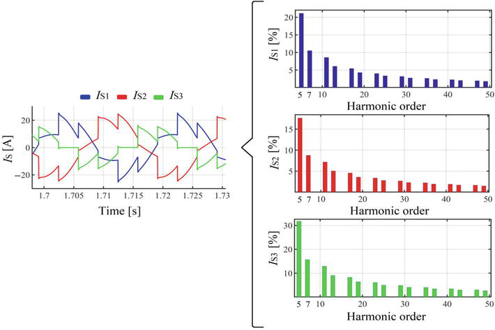
Figure 10.

Waveforms of the grid current with the spectrums before the SAPF connection.

4.3.1 Influence of the inverter input reactor size on the SAPF work efficiency

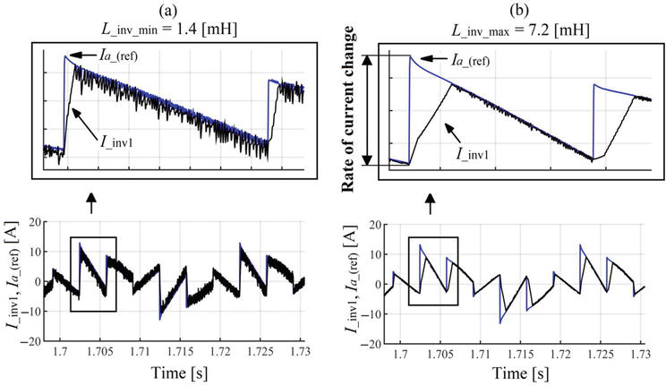
The goal of the investigation is to show how the size of the inverter input reactor has an influence on the SAPF work efficiency. For this purpose, two values of the inverter input reactor inductance are considered (Table 2): The first one ($L_{\_\mathrm{inv}\_min}=1.4\mathrm{mH}$) is obtained after assuming a minimum reactor voltage drop (e.g., $∆U_{\mathrm{L}\_\mathrm{inv}\_min}=3\mathrm{V}$) and the second one ($L_{\_\mathrm{inv}\_max}=7.2\mathrm{mH}$) after assuming a maximum reactor voltage drop (e.g., $∆U_{\mathrm{L}\_\mathrm{inv}\_min}=16\mathrm{V}$).

The grid voltage and current waveforms as well as the ones of the SAPF are presented respectively in Figures 11 and 12.

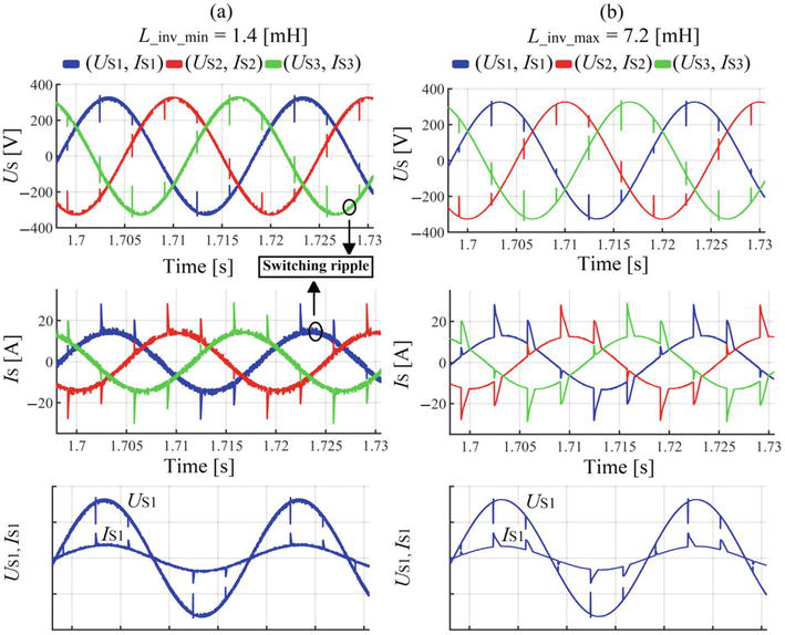
Figure 11.

Waveforms of the grid voltage and current after the SAPF connection: (a) for $L_{\_\mathrm{inv}\_min}$ and (b) for $L_{\_\mathrm{inv}\_max}$.

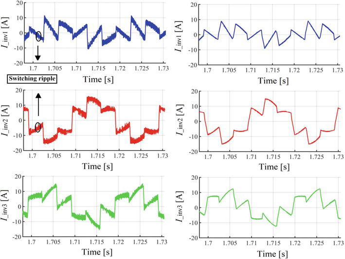
Figure 12.

Waveforms of the SAPF current: (a) for $L_{\_\mathrm{inv}\_min}$ and (b) for $L_{\_\mathrm{inv}\_max}$.

On the one hand, the SAPF with minimum input reactor inductance $L_{\_\mathrm{inv}\_min}$ (see Figures 11(a) and 12(a)) presents higher switching ripple components than the SAPF with the maximum input reactor inductance $L_{\_\mathrm{inv}\_max}$ (see Figures 11(b) and 12(b)). On the other hand, it presents better shape of the grid current waveforms at the commutation notches (comparing the grid current waveforms in Figure 11(a) to those in Figure 11(b)).

The grid voltage and current THD, powers, and asymmetry coefficient (${\mathrm{k}}_{\text{asym}}$) before the SAPF connection are presented in Table 4. In Table 5, it can be seen that the SAPF with $L_{\_\mathrm{inv}\_min}$ presents the lowest grid current and voltage THD as well as asymmetry coefficient. In Table 6, the SAPF with $L_{\_\mathrm{inv}\_max}$ has the lowest grid voltage true total harmonic distortion (TTHD) and the highest grid current TTHD (see (5)) in comparison with the SAPF with $L_{\_\mathrm{inv}\_min}$. The fundamental harmonic active, reactive, and apparent powers at the PCC, load, and SAPF are compared in Table 7.

	${\mathrm{THD}}_{\mathrm{US}}$ [%]	${\mathrm{THD}}_{\text{IS}}$[%]	$Q_{\mathrm{S}\left(1\right)}$[Var]	$P_{\mathrm{S}\left(1\right)}$[W]	$S_{\mathrm{S}\left(1\right)}$[VA]	${\mathrm{k}}_{\text{asym}}$ [%]
L1	0.25	28.07	414.08	2838.4	2868.5	33.25
L2	0.25	23.41	1954.5	2833.1	3441.9
L3	0.25	42.07	1181.8	1507.2	1915.2

Table 4.

Grid voltage and current parameters before the SAPF connection.

	$L_{\_\mathrm{inv}\_min}$ = 1.4 [mH]			$L_{\_\mathrm{inv}\_max}$ = 7.2 [mH]
	${\mathrm{THD}}_{\mathrm{US}}$ [%]	${\mathrm{THD}}_{\text{IS}}$[%]	${\mathrm{k}}_{\text{asym}}$ [%]	${\mathrm{THD}}_{\mathrm{US}}$ [%]	${\mathrm{THD}}_{\text{IS}}$[%]	${\mathrm{k}}_{\text{asym}}$ [%]
L1	0.18	10.34	0.59	0.25	26.7	0.75
L2	0.19	10.99		0.25	27.92
L3	0.18	10.93		0.25	27.7

Table 5.

Grid voltage and current parameters after the SAPF connection.

	After the SAPF connection
	$L_{\_\mathrm{inv}\_min}$ = 1.4 [mH]		$L_{\_\mathrm{inv}\_max}$ = 7.2 [mH]
	${\text{TTHD}}_{\mathrm{US}}$ [%]	${\text{TTHD}}_{\text{IS}}$[%]	${\text{TTHD}}_{\mathrm{US}}$ [%]	${\text{TTHD}}_{\text{IS}}$[%]
L1	3.57	16.31	1.70	27.09
L2	2.93	16.19	1.50	27.59
L3	3.60	16.20	2.13	27.89

Table 6.

PCC voltage and grid current TTHD.

		$L_{\_\mathrm{inv}\_min}$ = 1.4 [mH]			$L_{\_\mathrm{inv}\_max}$ = 7.2 [mH]
		PCC	Load	SAPF	PCC	Load	SAPF
$P_{\mathrm{S}\left(1\right)}$ [W]	L1	2411.4	2838.8	427.40	2389.3	2838.8	449.82
	L2	2535.8	2837.9	438.19	2416.8	2837.9	421.33
	L3	2522.3	1505.7	−890.35	2397.5	1505.7	−891.61
$Q_{\mathrm{S}\left(1\right)}$ [Var]	L1	46.30	414.13	370.22	91.78	414.13	323.23
	L2	57.54	1950.4	1898	97.07	1950.4	1854.5
	L3	39.62	1180.6	1143.7	117.25	1180.6	1062.6
$S_{\mathrm{S}\left(1\right)}$ [VA]	L1	2411.9	2868.8	565.46	2391.1	2868.8	553.92
	L2	2536.5	3443.5	1948	2418.8	3443.5	1.901.8
	L3	2522.6	1913.3	1449.4	2400.3	1913.3	1387.1

Table 7.

Active, reactive, and apparent powers at the PCC, load, and SAPF for the minimum and maximum input inverter reactor inductance.

$${\text{TTHD}}_{\text{Is}}=\frac{\sqrt{I_{\mathrm{S}\_\text{true}\_\mathrm{RMS}}^2-I_{\mathrm{S}\left(1\right)}^2}}{I_{\mathrm{S}\left(1\right)}}$$E5

An example of comparison waveforms between the reference current ($I_{a\_\left(\mathrm{ref}\right)}$) and the compensating current ($I_{\mathrm{inv}1}$) is presented in Figure 13(a) and (b). In the case of the SAPF with $L_{\_\mathrm{inv}\_min}$ (Figure 13(a)) as well as in the case of the SAPF with $L_{\_\mathrm{inv}\_max}$ (Figure 13(b)), the compensating current ($I_{\mathrm{inv}1}$) has difficulty to track the reference current ($I_{a\_\left(\mathrm{ref}\right)}$) at the points of commutation notches, due to the high rate of the reference current change at those points. That tracking difficulty is more accentuated in the case of the SAPF with $L_{\_\mathrm{inv}\_max}$ (Figure 13(b)) than in the case of the SAPF with $L_{\_\mathrm{inv}\_min}$ (Figure 13(a)). The high rate of current change observed on the reference current waveforms comes from the load current ($I_{\mathrm{T}}$). Because of the small size of the thyristor bridge input reactor $L_{\mathrm{T}}$, the rate of current change (di/dt) during commutation is high.

Figure 13.

Example of waveforms comparison between the reference and compensating currents (see control loop (3) in Figure 8): (a) for $L_{\_\mathrm{inv}\_min}$ and (b) for $L_{\_\mathrm{inv}\_max}$.

In this case study, it can be noticed that the gap between the reference current and the compensating current observed in Figure 13(a) and (b) is one of the factors that can influence the SAPF work efficiency, mostly in terms of current harmonics mitigation (see grid current THD in Table 5). That gap is responsible for the high amplitude ripples at the points of commutation notches observed on the grid current waveform in Figure 11(b).

It has been clearly demonstrated that the size of the SAPF input reactor affects its work efficiency. The SAPF with big size of input reactor has showed a better result in terms of inverter switching ripples reduction but worst result in terms of reducing the ripples caused by the high rate of current change during the commutation. In contrary to the SAPF with big size reactor, the SAPF with small size of input reactor has showed a worst result in terms of inverter switching ripples reduction but a better result in terms of ripple reduction at the high rate of current change during the commutation. At the grid side, the SAPF with small inductance (${\mathit{L}}_{\_\mathrm{inv}\_min}$) has showed better results in terms of THD (TTHD current), asymmetry coefficient, and reactive power compensation (Table 7) at the grid side. The SAPF with big reactor inductance (${\mathit{L}}_{\_\mathrm{inv}\_max}$) has showed better results in terms of TTHD of the PCC voltage.

4.3.2 Influence of the thyristor bridge input reactor size on the SAPF work efficiency

This investigation is performed because of the problem of ripples reduction due to the high rate of load current change observed in the previous investigations. The goal is to demonstrate that the SAPF input reactor size should be chosen by considering also the thyristor bridge input reactor size in order to improve the SAPF work efficiency.

The SAPF parameters are constant during the investigation. The value of the SAPF input reactor inductance ($L_{\_\mathrm{inv}\_min}=1.4\mathrm{mH}$) is chosen based on the previous investigation. The only load parameter changing is the input reactor $L_{\mathrm{T}}$ (0.25, 1.4, or 3 mH). Three case studies are compared: (a) The SAPF input reactor inductance is higher than the thyristor-bridge input reactor inductance ($L_{\_\mathrm{inv}\_min}>L_{\mathrm{T}}$), (b) the SAPF input reactor inductance is equal to the thyristor-bridge input reactor inductance ($L_{\_\mathrm{inv}\_min}=L_{\mathrm{T}}$), and (c) the SAPF input reactor inductance is smaller than the thyristor-bridge input reactor inductance ($L_{\_\mathrm{inv}\_min}<L_{\mathrm{T}}$).

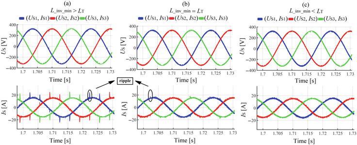
The grid voltage and current waveforms in Figure 14 show that in the cases of SAPF with the input reactor inductance equal or smaller than thyristor bridge input reactor, the ripples caused by the high rate of current change at the points of commutation notches are better reduced (see current waveform in Figure 14(b) and (c)). The case in which $L_{\_\mathrm{inv}\_min}<L_{\mathrm{T}}$ presents the best shape of grid current waveforms (Figure 14(c)).

Figure 14.

Waveforms of PCC voltage and current for different value of the thyristor bridge input reactor: (a) $L_{\_\mathrm{inv}\_min}>L_{\mathrm{T}}$, (b) $L_{\_\mathrm{inv}\_min}=L_{\mathrm{T}}$, (c) $L_{\_\mathrm{inv}\_min}<L_{\mathrm{T}}$.

In Table 8, it can be observed that the best results in terms of grid voltage and current THD as well as asymmetry mitigation are when $L_{\_\mathrm{inv}\_min}\le L_{\mathrm{T}}$. Observing the grid powers in Table 9, it can be seen that the case with $L_{\_\mathrm{inv}\_min}<L_{\mathrm{T}}$ has the best reactive power compensation.

	Before the SAPF connection			After the SAPF connection
	$L_{\mathrm{T}}$ = 1 nH			$L_{\_\mathrm{inv}\_min}$ > $L_{\mathrm{T}}$
	${\mathrm{THD}}_{\mathrm{US}}$ [%]	${\mathrm{THD}}_{\text{IS}}$[%]	${\mathrm{k}}_{\text{asym}}$ [%]	${\mathrm{THD}}_{\mathrm{US}}$ [%]	${\mathrm{THD}}_{\text{IS}}$[%]	${\mathrm{k}}_{\text{asym}}$ [%]
L1	0.25	28.07	33.25	0.15	8.77	0.30
L2	0.25	23.41		0.15	8.75
L3	0.25	42.07		0.15	8.77
	After the SAPF connection
	$L_{\_\mathrm{inv}\_min}$ = $L_{\mathrm{T}}$			$L_{\_\mathrm{inv}\_min}$ < $L_{\mathrm{T}}$
	${\mathrm{THD}}_{\mathrm{US}}$ [%]	${\mathrm{THD}}_{\text{IS}}$[%]	${\mathrm{k}}_{\text{asym}}$ [%]	${\mathrm{THD}}_{\mathrm{US}}$ [%]	${\mathrm{THD}}_{\text{IS}}$[%]	${\mathrm{k}}_{\text{asym}}$ [%]
L1	0.04	2.47	0.30	0.02	1.22	0.20
L2	0.05	2.91		0.02	1.49
L3	0.05	2.79		0.02	1.22

Table 8.

Grid voltage and current THD as well as asymmetry coefficient before and after the SAPF connection.

	Before the SAPF connection		After the SAPF connection
	$L_{\mathrm{T}}$ = 1 nH		$L_{\_\mathrm{inv}\_min}$ > $L_{\mathrm{T}}$
	$Q_{\mathrm{S}\left(1\right)}$[Var]	$P_{\mathrm{S}\left(1\right)}$[W]	$Q_{\mathrm{S}\left(1\right)}$[Var]	$P_{\mathrm{S}\left(1\right)}$[W]
L1	414.08	2838.4	25.15	2402.5
L2	1954.5	2833.1	33.51	2400.1
L3	1181.8	1507.2	29.24	2393.2
	After the SAPF connection
	$L_{\_\mathrm{inv}\_min}$ = $L_{\mathrm{T}}$		$L_{\_\mathrm{inv}\_min}$ < $L_{\mathrm{T}}$
	$Q_{\mathrm{S}\left(1\right)}$[Var]	$P_{\mathrm{S}\left(1\right)}$[W]	$Q_{\mathrm{S}\left(1\right)}$[Var]	$P_{\mathrm{S}\left(1\right)}$[W]
L1	24.86	2374.8	20.42	2340.2
L2	29.04	2377.1	28.59	2340.1
L3	28.98	2372.4	24.43	2333.3

Table 9.

Grid voltage and current reactive and active power before and after the SAPF connection.

The TTHD of the grid voltage and current are presented in Table 10. The case with $L_{\_\mathrm{inv}\_min}<L_{\mathrm{T}}$ presents the best result in terms of current ${\text{TTHD}}_{\text{IS}}$ and the worst results in terms of voltage ${\text{TTHD}}_{\mathrm{US}}$.

	After the SAPF connection
	$L_{\_\mathrm{inv}\_min}$ > $L_{\mathrm{T}}$		$L_{\_\mathrm{inv}\_min}$ = $L_{\mathrm{T}}$		$L_{\_\mathrm{inv}\_min}$ < $L_{\mathrm{T}}$
	${\text{TTHD}}_{\mathrm{US}}$ [%]	${\text{TTHD}}_{\text{IS}}$[%]	${\text{TTHD}}_{\mathrm{US}}$ [%]	${\text{TTHD}}_{\text{IS}}$[%]	${\text{TTHD}}_{\mathrm{US}}$ [%]	${\text{TTHD}}_{\text{IS}}$[%]
L1	3.12	12.60	3.18	7.16	3.30	6.59
L2	2.77	13.77	2.85	8.08	2.92	6.82
L3	3.12	13.40	3.23	7.20	3.29	6.11

Table 10.

PCC voltage and grid current TTHD for different value of thyristor bridge input reactor inductance.

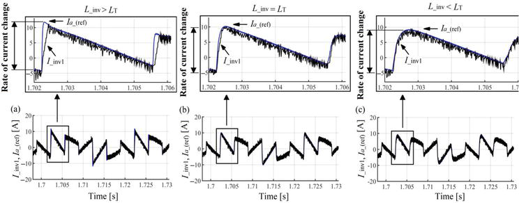
The waveforms of the reference current compared to the ones of the compensating current are presented in Figure 15. It can be seen that in the case of $L_{\_\mathrm{inv}\_min}<L_{\mathrm{T}}$, the reference current and the compensating current match each other (Figure 15(c)). The increase of the thyristor-bridge input reactor inductance $L_{\mathrm{T}}$ to a value equal or higher than the SAPF input reactor inductance ($L_{\_\mathrm{inv}\_min}$) has reduced the rate of current change at the points of commutation notches making possible the tracking of the reference current by compensating current (Figure 15(b) and (c)).

Figure 15.

Waveforms comparison between the reference and compensating current: (a) $L_{\_\mathrm{inv}\_min}>L_{\mathrm{T}}$, (b) $L_{\_\mathrm{inv}\_min}=L_{\mathrm{T}}$, (c) $L_{\_\mathrm{inv}\_min}<L_{\mathrm{T}}$.

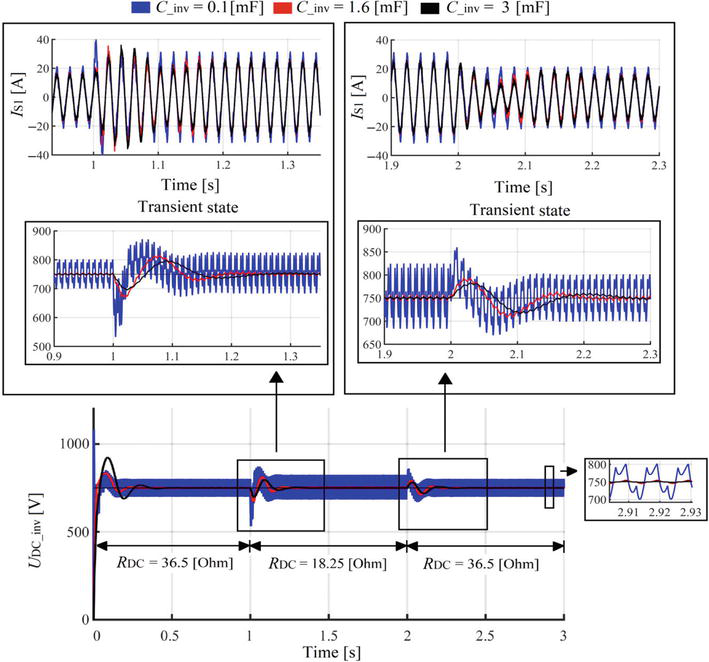
Figure 16 presents the SAPF DC capacitor voltage for different values of capacity. It can be also observed the ability of the control system algorithm in response to the decrease and increase of the thyristor-bridge DC resistance (load change).

Figure 16.

Capacitor DC voltage waveforms for different capacitance: Transient state observation after the thyristor-bridge DC resistance change (R_DC).

The investigations have clearly showed that the size of the thyristor-bridge input reactor has an influence of the SAPF work efficiency. The SAPF with the input reactor inductance equal or smaller than the one at the thyristor-bridge input has presented the best results in terms of grid voltage and current THD as well as in terms of reactive power and asymmetry mitigation. The inductance of the SAPF input reactor should be computed or chosen considering the size of the thyristor-bridge input reactor (see expression (6)). $∆U_{\mathrm{L}\_\mathrm{inv}}$ should be chosen in such a way to obtain $L_{\_\mathrm{inv}}\le L_{\mathrm{T}}$.

$$L_{\_\mathrm{inv}}=\frac{3∆U_{\mathrm{L}\_\mathrm{inv}}}{{\mathrm{\omega }}_{\left(1\right)}\left(I_{a\_\left(\mathrm{ref}\right)}+I_{b\_\left(\mathrm{ref}\right)}+I_{c\_\left(\mathrm{ref}\right)}\right)}\le L_{\mathrm{T}}$$E6

5. Investigation on the work efficiency of the SHAPF

In the chapter, the investigation of the SHAPF work efficient is focused on the tuning frequency of the passive part (balance load). The passive part is tuned to three different frequencies and the results in terms of grid voltage and current THD, waveforms and powers are compared. The influence of the thyristor bridge input reactor on the choice of the passive part tuning frequency is presented as well as the limitation of such topology in terms of asymmetry compensation. It is also demonstrated that the grid dependency of the passive part work efficiency in terms of harmonics mitigation (see investigation in Chapter 3) is eliminated as well as the parallel resonance between the passive part and the grid.

5.1 Functionality principle of the SHAPF

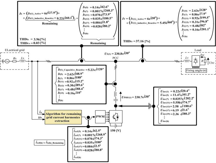
The SHAPF work principle is presented in Figure 17. The load is symmetrical and is the source of distorted current, which is composed of three components: active ($I_{\mathrm{T}\left(1\right)\_\text{Active}}$), inductive reactive ($I_{\mathrm{T}\left(1\right)\_\text{Inductive}\_\text{Reactive}}$), and harmonics ($I_{\mathrm{T}\left(\mathrm{h}\right)}$). The SHAPF passive part is tuned to the frequency of 7th harmonic just to illustrate the SHAPF functionality principle.

Figure 17.

SHAPF work principle.

The role of the passive part is to compensate the load fundamental harmonic reactive power by producing through its capacitor a capacitive reactive current ($I_{\mathrm{f}\left(1\right)\_\text{Capacitive}\_\text{Reactive}}$) which at the PCC cancel with the load inductive reactive current ($I_{\mathrm{T}\left(1\right)\_\text{Inductive}\_\text{Reactive}}$). In Figure 17, it can be seen that, the load inductive reactive current which was 5.45 A is reduced to 0.22 A at the grid side. It plays also the role of the inverter switching ripples attenuation mostly through its reactor. It has small impedance for the resonance frequency and frequencies around.

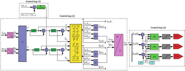
The SHAPF proposed control system is designed without any feedback signal coming from the inverter AC side (see Figures 17 and 18). As in the case of the SAPF control system (see Figure 8), it contains also three control loops ((1) to (3)). Its algorithm (based on the instantaneous p-q theory) computes the reference current ($I_{f\left(\mathrm{h}\right)}$) using the grid current remaining harmonics ($I_{\mathrm{S}\left(\mathrm{h}\right)\text{Remaining}}$). Therefore based on the reference harmonics current $I_{\mathrm{ref}\left(\mathrm{h}\right)}$(e.g., $I_{\mathrm{ref}\left(5\right)}=0.14e^{j{42.5}^{°}}$), the inverter generates current harmonics $I_{\mathrm{f}\left(\mathrm{h}\right)}$ (e.g., $I_{\mathrm{f}\left(5\right)}=2.62e^{-j{48.9}^{°}}$) with the same amplitudes and angle as the load current harmonics (e.g., $I_{\mathrm{T}\left(5\right)}=2.63e^{j{128}^{°}}$) but in opposite sign so that they cancel each other at the PCC (the grid current THD is reduced from 37.16 to 3.96%—Figure 17). The inverter behaves like a harmonics voltage source (see $U_{\mathrm{inv}\left(\mathrm{h}\right)}$ in Figure 17). At the grid side, it can be noticed a current ($I_{\mathrm{S}}$) with almost not-change in the active component ($I_{\mathrm{S}\left(1\right)\_\text{Active}}$) and with the remaining reactive and harmonic components (see Figure 17).

Figure 18.

Block diagram of the SHAPF control system: a, b, and c—Phase designations of the supply network; 1, 2, and 3—represent the inverter inputs.

5.2 HAPF simulation studies

Three simulation case studies are investigated and compared: In the first one, the SHAPF passive part is tuned to the frequency lower (e.g., 4.87) than the frequency of the first load characteristic harmonic (the 5th); in the second one, it is tuned to the frequency lower (e.g., 6.87) than the frequency of the second load characteristic harmonic (the 7th), and in the third one, it is tuned to the frequency lower (e.g., 10.87) than the frequency of the third load characteristic harmonic (the 11th).

5.2.1 Simulation assumption

In the electrical system (see Figure 1), k1 is closed ($L_{\mathrm{SS}}$ is not considered), the load (k5 open) and the SHAPF control system parameters are constant, the load input reactor resistance as well as the ones of the passive part capacitor and inverter DC capacitor are neglected, k2 and k3 are opened, and k4 is close. The DC voltage of the active part is 150 V. The only parameter changing is the tuning frequency of the filter passive part. Because of the symmetrical power system, some results are presented only for one-phase.

5.2.2 SHAPF parameters computation

The SHAPF and the load ($Q_{\mathrm{f}}=Q_{\mathrm{T}}$, $L_{\mathrm{T}}$) parameters are shown in Table 11. The passive part parameters are computed based on the formula presented in Figure 4(a). Observing Table 11, it can be seen that, with the resonance frequency increase from 4.87 to 10.87, the passive part reactor inductance has decreased, whereas its capacitor capacity has increased. From the cost and power losses point of view, the PHF with the resonance frequency ($n_{\mathrm{re}}=10.87$ (543.5 Hz)) near the frequency of the 11th harmonic presents less exploitation cost and will generate less power losses because of its lowest equivalent resistance value.

$n_{\mathrm{re}}$	$L_{\mathrm{f}}$ [mH]	$C_{\mathrm{f}}$ [μF]	$R_{\mathrm{Lf}}$ [mΩ]	$Q_{\mathrm{f}}$ [Var]	$q_{\mathrm{Lf}}$	$L_{\mathrm{T}}$ [mH]	$U_{\mathrm{DC}\_\mathrm{inv}}$ [V]
4.87	6.1	69.74	12.8	1210	150	3.5	150
6.87	3.0	71.27	6.3
10.87	1.2	72.19	2.5

Table 11.

SHAPF parameters.

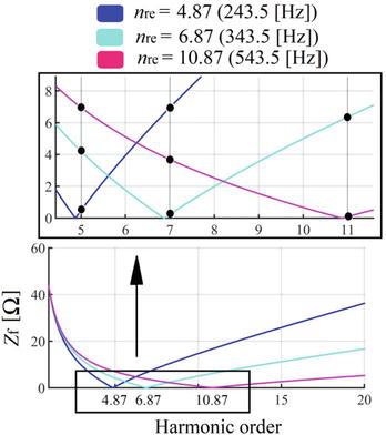
Table 12 presents the electrical grid and SHAPF passive part equivalent impedances of the 5th, 7th, and 11th harmonics. The grid equivalent impedances for the 5th and 7th harmonics are smaller than the ones of the SHAPF passive part and concerning the 11th harmonic, the situation is contrary (see Table 12). The passive part impedance versus frequency characteristics are presented in Figure 19.

${\mathit{Z}}_{\mathbf{S}\left(\mathbf{5}\right)}$ [mΩ]	${\mathit{Z}}_{\mathbf{\text{SHAPF}}\left(\mathbf{5}\right)}$ [mΩ]	${\mathit{Z}}_{\mathbf{S}\left(\mathbf{7}\right)}$ [mΩ]	${\mathit{Z}}_{\mathbf{\text{SHAPF}}\left(\mathbf{7}\right)}$ [mΩ]	${\mathit{Z}}_{\mathbf{S}\left(\mathbf{11}\right)}$ [mΩ]	${\mathit{Z}}_{\mathbf{\text{SHAPF}}\left(\mathbf{11}\right)}$ [mΩ]
49.5	490	69.2	243	108.8	96.4

Table 12.

Electrical grid and SHAPF passive part equivalent impedance of the 5th, 7th, and 11th harmonics (the line reactor $L_{\mathrm{SS}}$ is not considered).

Figure 19.

SHAPF passive part impedance versus frequency characteristics.

5.2.3 Simulation results

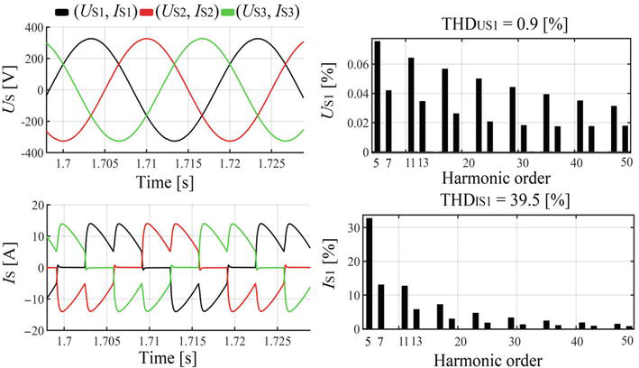
The grid voltage and current waveforms with the spectrums before the SHAPF connection are presented in Figure 20. Because of the electrical grid rigidity (very small inductance), the PCC voltage waveforms are almost not distorted.

Figure 20.

Grid voltage ($U_{\mathrm{S}}$) and current ($I_{\mathrm{S}}$) waveforms with their spectrums before the SHAPF connection.

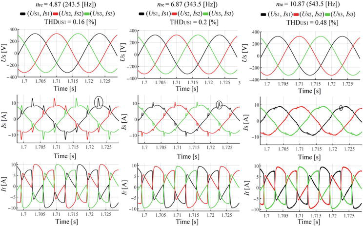
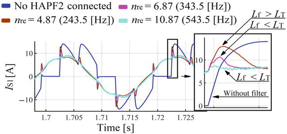
In Figure 21, the waveforms of the grid voltage ($U_{\mathrm{S}}$) and current ($I_{\mathrm{S}}$) as well as SHAPF current ($I_{\mathrm{f}}$) after the SHAPF connection are presented. It can be noticed that the SHAPF with the passive part tuned to the frequency (e.g., 543.5 Hz, 10.87) a bit lower than the frequency of the 11th harmonic presents the best reduction of the grid current ripples at the high rate of current change points (see commutation points on the grid current waveforms ($I_{\mathrm{S}}$) in Figure 21), although it presents the highest PCC voltage THD (Figure 21).

Figure 21.

Waveforms of grid voltage ($U_{\mathrm{S}}$) and current ($I_{\mathrm{S}}$) and SHAPF current ($I_{\mathrm{f}}$) for the PHF tuned to the harmonic component frequency of order 4.87, 6.87, and 10.87.

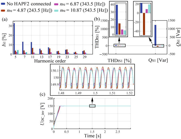
In the comparison spectrum of the grid current presented in Figure 22(a), the SHAPF with the PHF tuned to the harmonic component frequency of 10,87 presents the best reduction of the higher harmonics starting from the 11th (according to the characteristics in Figure 19, the PHF presents the lowest impedance for the higher harmonics) as well as the lowest ${\mathrm{THD}}_{\text{IS}}$(see Figure 19(b)). But it presents the highest 5th harmonic impedance (see Figure 19) and for that reason the 5th harmonic is worst reduced at the grid side (Figure 22(a)).

Figure 22.

(a) Grid current spectrum, (b) grid current THD and fundamental harmonic reactive power, and (c) SHAPF DC voltage.

The SHAPF with the PHF tuning frequency ($n_{\mathrm{re}}=6.87$) around the frequency of the 7th harmonic presents the lowest amplitude of the grid current 5th and 7th harmonics (Figure 22(a). Despite the fact that the grid equivalent impedances of the 5th and 7th harmonics are smaller than the ones of the SHAPF passive part (See Table 12), those harmonics are considerably reduced at the grid side after the SHAPF connection (see spectrum in Figure 22(a)) and this shows that the grid dependency of the PHF work efficiency is eliminated. The inverter through its control system has improved the passive part work efficiency in terms of harmonics filtration.

In Figure 22(b), it can also be noticed that the PCC fundamental harmonic reactive power ($Q_{\mathrm{S}}$) is the best compensated for the SHAPF with the PHF tuned to the harmonic component frequency of 6.87 (near the 7th).

The difference observed in the results of the grid fundamental reactive powers after the SHAPF connection in Figure 22(b) is due to the fact that, for different PHF tuning frequency, the SHAPF has generated different fundamental harmonic reactive power (a bit different than the one used to compute the PHF parameters in Table 11) for the compensation at the PCC (see $Q_{\mathrm{f}\left(1\right)}$ in Table 13).

	No filter	$n_{\mathrm{re}}$ = 4,87	$n_{\mathrm{re}}$ = 6,87	$n_{\mathrm{re}}$ = 10,87
$Q_{\mathrm{S}1\left(1\right)}$[Var]	1234	−48.7	8,16	18,31
$P_{\mathrm{S}1\left(1\right)}$) [W]	1435	1438	1437	1435
$Q_{\mathrm{f}1\left(1\right)}$ [Var]	—	−1283	−1226	−1216
$S_{\mathrm{f}1\left(1\right)}$ [VA]	—	1282,83	1225,70	1217,54
$P_{\text{load}1\left(1\right)}$ [W]	—	1437	1437	1437
$Q_{\text{load}1\left(1\right)}$ [Var]	—	1234	1234	1234

Table 13.

One-phase representation of the fundamental harmonic active, reactive, and apparent powers at the load, SHAPF, and grid side.

In comparison with the SAPF DC voltage (which is around 750 V in Figure 16), the SHAPF inverter DC voltage in Figure 22(c) is five times smaller (150 V).

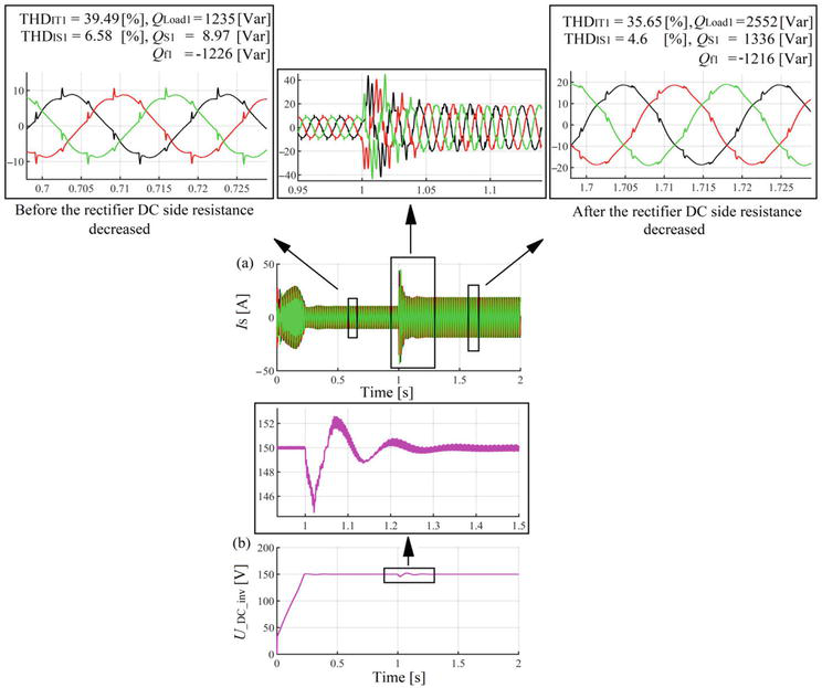
The ability of the SHAPF control system to compensate harmonics after the load change is presented in Figure 23(a) (see grid current waveforms $I_{\mathrm{S}}$). The load DC resistance is changed from 36.5 to 18.25 Ω and the inverter DC voltage is presented in Figure 23(b). Observing the zooms in Figure 23(a), it can be noticed that after the load change, the grid current harmonics are well reduced (${\mathrm{THD}}_{\text{IS}}$ is reduced from 36.65 to 4.6%), but the grid fundamental reactive power ($Q_{\mathrm{S}1}$) is partially compensated (from 2552 to 1336 Var) because of the fixed SHAPF passive part reactive power (1210 Var see Table 11). This is one of the disadvantages of such SHAPF topology.

Figure 23.

(a) Grid current waveforms and (b) SHAPF DC voltage before and after the load change ($\mathrm{R}$dc is changed from 36.5 to 18.25 Ω).

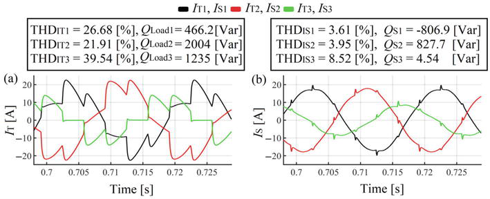
Figure 24(a)(b) presents the grid and load current waveforms respectively during the asymmetry (k5 closed—see Figure 1). It can be noticed that the SHAPF with the proposed control system (see Figure 18) does not have ability to compensate the asymmetry component. This is another disadvantage of such SHAPF topology.

Figure 24.

Unbalance load (k5 closed—see Figure 1): Waveforms of the load current (a) and grid current (b).

The power system impedance versus frequency characteristic observed from the thyristor bridge input is presented in Figure 25. On that characteristic, it can be noticed no resonance phenomena (parallel and series) contrary to the case of the characteristics in Figure 7. The parallel resonance between the PHF (when operating alone) and the electrical gird is eliminated as well as the grid dependency of the PHF work efficiency (when operating alone).

Figure 25.

Frequency impedance characteristic of the power system seen from thyristor bridge input (k1 closed).

Figure 26 presents the grid current waveforms before and after the SHAPF connection. It can be noticed that the ripples at the high rate of current change (see zoom Figure 26) are better mitigated when the passive part is tuned to the frequencies of 243.5 and 543.5 Hz, respectively, near to the frequencies of the 7th and 11th harmonics (see grid current waveforms in Figure 21). Observing Table 11, it can be seen that with those frequencies, the passive part reactor inductance ($L_{\mathrm{f}}$) is smaller than the thyristor bridge input reactor inductance ($L_{\mathrm{T}}$). Therefore, in this case study, the SHAPF passive part tuning frequency should be chosen taking also into account the size of the thyristor bridge input reactor which should be higher for a better ripple mitigation at the commutation points.

Figure 26.

Waveforms of the grid current before and after the SHAPF connection.

The performed studies have shown that when the SHAPF passive part is tuned to the frequency of harmonic higher than the 5th and 7th harmonics: the higher grid current harmonics (e.g., from the 13th) are better reduced because the PHF presents smaller impedance for those harmonics, the 5th and 7th harmonics currents are worse reduced, and the PHF reactor size is smaller therefore low cost. In the case where the passive part reactor size is smaller than the one at the thyristor bridge input, the switching ripple are worst mitigated, but the ripples at the commutation points are better mitigated.

6. Conclusion

The detail investigations on the PHF, SAPF, and HAPF work efficiency have been presented in this chapter. They were performed in the electrical system with six-pulse thyristor-bridge as load. The first investigation concerned the grid dependency of the PHF work efficiency in terms of harmonics mitigation. And it has been recommended the use an additional line reactor between the PCC and the filter to increase the PHF effectiveness in terms of harmonics mitigation.

In the second one, the influence of the thyristor-bridge input reactor size on the SAPF work efficiency was studied. And it has been recommended to choose or compute the SAPF input reactor parameters taking also into account the thyristor bridge input reactor size. According to that investigation, the SAPF input reactor inductance should be equal or smaller than the one at the thyristor bridge input for good work efficiency.

The last investigation was related to the SHAPF, comparing its work efficiency for different tuning frequencies. It has been demonstrated that for a better ripple reduction at commutation points, the passive part tuning frequency should be chosen in such a way that the filter reactor inductance is smaller than the one of the thyristor bridge input reactor. With the inverter connected in series with the PHF, the grid dependency of the PHF work efficiency is eliminated as well as the parallel resonance that could occurred between the grid and PHF. One of the useful advantages in that topology is that the SAPF DC voltage can be considerably reduced in comparison with the case when it is operating alone. The main disadvantages of such topology are that it has fixed compensating reactive power and presents difficulty to compensate asymmetry component.

Conflict of interest

The authors declare no conflict of interest.