The Finite Fractal Distributions as Mean Grain Size Distributions of Granular Matter

Abstract

The grading entropy is the statistical entropy of the finite discrete grain size distribution on N uniform statistical cells in terms of the N sieve cells, consisting of two terms, the base entropy and the entropy increment (depending on N), which have normalized forms as well (basically independent of N). Being the most adequate statistical variables, both physical phenomena and physical model parameters can be best described by their use. Among others, the normalized base entropy A can be used to measure internal stability, being related to erosion, piping and liquefaction phenomena. Its value classifies the grading curves. Each class (with a fixed value of A) has a mean grading curve with finite fractal distribution, the fractal dimension varies from minus to plus infinity. (These mean gradings indicate a unique relation between the four entropy coordinates and four central moments). The internally stable fractal dimensions - between 2 and 3 – are occurring in nature verifying the internal stability rule of grading entropy. The widespread fractal soils are formed by degradation, which has a directional grading entropy path, with different features in terms of non-normalized and normalized grading entropy coordinates.

1. Introduction

The grading curves contain a large amount of data. Hence, definitions and rules based on a few specified particle diameters are used in practice. For example, considering the diameter values (d), the range of gravel is d = 2 to 64 mm, the range of sand is d = 0.06 to 2 mm and the range of silt is d = 0.002 to 0.06 mm. These statistical cell sizes indicate that the probability variable is the logarithm of d (since the sieve hole diameters are doubled).

The coefficient of uniformity (C_U = d₆₀/d₁₀) and the coefficient of curvature (C_C = d₃₀²/(d₆₀d₁₀)) are frequently used. A granular soil is considered well-graded if C_U > 4 and 1 < C_c < 3, otherwise it is poorly graded. These descriptors can provide limited information and these approaches are not valid for gap-graded grain size distributions. The use of these is somewhat controversial, since the grading curve is generally represented in terms of the logarithm of d.

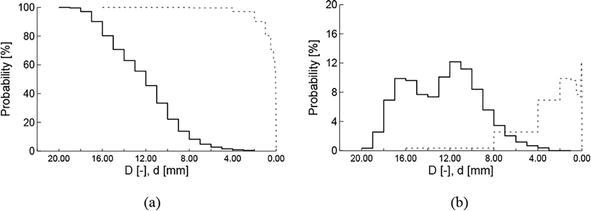
Statistically, the measured grading curve is a finite, discrete distribution curve with N uniform statistical cells in terms of the logarithm of diameter d (N sieves, Figure 1). The distributions are frequently gap-graded or bimodal, and, the four central moments in terms of the logarithm of diameter d are with limited use except the mean. Therefore, the most adequate statistical variables are the grading entropy coordinates.

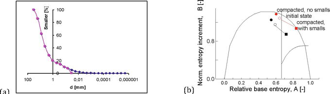
Figure 1.

(a, b): Grain size distribution function and density function in terms of diameter d (dashed line) and in terms of a kind of logarithm of d variable denoted by D (integer variable, solid line).

The grading entropy is the statistical entropy of the finite discrete grain size distribution on N uniform statistical cells in terms of the N sieve cells, consisting of two terms, the base entropy and the entropy increment (depending on N), which have normalized forms as well (basically independent of N). Both physical phenomena and physical model parameters can be best described by their use. Moreover, the four central moments in terms of the logarithm of diameter d are with limited use except for the mean, since the distributions are frequently gap-graded or bimodal. The grading entropy coordinates ([1], see the history in the Appendix) can be used for gap-graded or bimodal mixtures, the represent of the grading curve (path) in the 2-dimensional space, to elaborate the rules e.g., for internal stability, segregation and filtering in the grading entropy diagram [1], to study degradation or soil maturing.

The content of the chapter is as follows: The normalized grading entropy coordinates can be used to classify the grain size distribution curves (on the basis of the internal stability rule and their degradation lifetime), to define a mean grading curve with fractal distribution in each class [2]. The mean grading curves can be used to clarify the mean relationships between the various statistics of the grading curves [3]. The grading entropy coordinates can be used to extend the present liquefaction, erosion and piping rules into a more general form. The grading entropy coordinates can be used to study the degradation or breakage process [4], and to represent the degradation of various rock material tests on the same diagram [5] where the internal stability rules are represented. The results of these tests indicate that there is a unique, material-independent entropy path at a given testing condition with directional properties. The natural soils are internally stable due to the entropy path of the degradation [6].

The grading entropy coordinates have many other uses (not treated here) e.g., in the explanation of dry density of granular matter, for soil classification and in the interpolation of functions between the model parameters and the grading curve, where the fractal grading curves have also importance in the experimental testing since these are mean grading curves.

2. Grading entropy

2.1 Entropy of a statistical distribution

Let us consider M elements in m cells and, M_i elements in the i-th cell. The statistical entropy S_s is [7]:

$$S_s=\mathit{Ms},$$E1

where s is the specific entropy or the entropy of an element given by

$$s=-\sum _{i=1}^m{\alpha }_i{log}_b{\alpha }_i$$E2

In eq. (2), b is the base of the logarithm, and α_i is the relative frequency of the i-th cell, given by

$${\alpha }_i=\frac{M_i}{M}$$E3

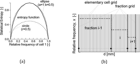
Let us consider two statistical cells, with relative frequencies of α₁ and α₂ = 1-α₁. If the base of the logarithm is set to 2 in Eq. (2) then the maximal specific entropy of this system is equal to 1 at the point α₁ = α₂ = 0.5 (Figure 2(a)). In the following, the base of the logarithm will be considered to be equal to 2. The specific entropy is written as follows, using b = 2, when the maximum ordinate is equal to 1:

Figure 2.

(a) The entropy function of two cells, N = 2. (b) the fractions and the elementary cell grid, assuming uniform distribution within the fractions.

$$s=-\frac{1}{ln2}\sum _{i=1}^m{\alpha }_{i}ln{\alpha }_i$$E4

As it will be shown later on, this function – being similar to a half-ellipse – determines the shape of the boundary lines of the entropy diagram for small N (see Section 3.2).

2.2 Statistical cells for the grading entropy

The statistical entropy of the grading curve is derived [1] from the definition of the entropy of a finite, discrete distribution [2], assuming a double cell system, the N “fractions” (uniform cell system in terms of logarithm of d) are embedded into the uniform elementary cell system in terms of d, defining a smallest diameter value d₀.

The statistical entropy formula is based on a uniform cell system. However, the measurement (using the sieve hole diameters) is made in a cell system uniform in the log d scale. Therefore, a double-cell system is used. The primary statistical cells or fractions are defined by successive multiplication with a factor of 2, starting from an (arbitrary) elementary cell width d₀ [8], the diameter range for fraction j:

$$2^{j+1}{d}_0\ge d>2^j{d}_0$$E5

where d₀ is the elementary cell width (Table 1). Its possible value is equal to the height of the SiO₄ tetrahedron (d₀ = 2⁻²² mm [9]). The number of the fractions N is the difference between the serial numbers of the finest and coarsest fractions as follows:

k	1	..	23	24
Limits	d0 to 2 d0	..	2^22d0to 2^23d0	2^23d0 to 2^24d0
S0k or D [−]	1	..	23	24

Table 1.

Definition of fractions serial numbers and fraction entropies.

$$N=j_{\max }-j_{\min }+1.$$E6

A secondary cell system is defined with equal width of d₀, assuming that the distribution is uniform within a fraction. The number of the elementary cells C_i in fraction i is equal to:

$$C_i=\frac{2^{i+1}{d}_{\min }-2^i{d}_{\min }}{d_{\min }}=2^i$$E7

The relative frequency of an elementary cell in fraction i is equal to:

$${\alpha }_i=\frac{x_i}{C_i}$$E8

where x_i is the relative frequency of fraction i.

2.3 The definition of the grading entropy coordinates

The grading entropy S is the statistical entropy of the grading curve in terms of the elementary statistical cells (the statistical specific entropy of the grading curve in terms of the elementary cells). By inserting the relative frequency of the secondary cell α_i (i.e., Eq. (8)) into Eq. (4), the grading entropy S can be derived:

$$S=-\frac{1}{ln2}\sum _{k=i_1}^{i_N}{x}_{k}ln{x}_k+\sum _{k=i_1}^{i_N}{x}_k\frac{ln{C}_k}{ln2}S=\mathrm{\Delta }S+S_o$$E9

It can be split into the base entropy S₀ and the entropy increment ΔS:

$$S_o=\sum _{i=1}^N{x}_i{S}_{\mathit{oi}}\text{and}\mathit{\Delta S}=-\frac{1}{ln2}\sum _{i=1}^N{x}_{i}ln{x}_i$$E10

$$S_{\mathit{oi}}=\frac{ln{C}_i}{ln2},S_{\mathit{oi}}=\frac{ln{2}^i}{ln2}=i$$E11

where S_0k (=D_k) is the grading entropy of the k-th fraction (Table 1), which is a positive integer, as it can be derived from Eqs. (7) and (10). It is uniquely related to logarithm of d, monotonically increasing with d (being about equal to the sieve or fraction serial number), expressing that the fraction cells are wider with d.

The base entropy S₀ is the mean fraction entropy weighed by the relative frequencies. The normalized base entropy, the so-called relative base entropy A:

$$A=\frac{S_o-S_{\mathit{\text{omin}}}}{S_{\mathit{\text{omax}}}-S_{\mathit{\text{omin}}}},A=\frac{\sum _{i=1}^N{x}_i\left(S_{\mathit{oi}}-S_{omin}\right)}{N-1}=\frac{\sum _{i=1}^N{x}_i\left(i-1\right)}{N-1}.$$E12

The entropy increment ΔS is a smooth, concave function on the open simplex which may continuously be extended to the closed simplex. The normalized entropy increment B is defined as follows:

$$B=\frac{\mathit{\Delta S}}{lnN}$$E13

The range of the entropy coordinates is dependent on N, ΔS varies between 0 and lnN/ln2 and S₀ varies between S_0min and S_0max. The normalized coordinates are independent of the selection of d₀. The normalized coordinate B varies between 0 and 1/ln2 and the relative base entropy A between 0 and 1.

3. The grading entropy map

3.1 The definitions

The spaces of the possible grading curves consist of such finite, discrete grain size distributions, which are composed of the same N consecutive fractions with minimum grain diameter d_min (being larger than or equal to d₀). The sum of the N relative frequencies x_i (i = 1, 2, 3...N) is equal to 1:

$$\sum _{\mathrm{j}=1}^{\mathrm{N}}{x}_j=1,x_j\ge 0$$E14

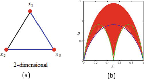
Eq. (14) is the equation of an N-1 dimensional closed simplex (Figure 3(a)), the N-1 dimensional analogy of the triangle or tetrahedron (i.e., the 2- and 3-dimensional instances) and the x_i (i = 1, 2, 3...N). The i-th barycentre coordinate (distance of the face generated by vertices 1…i-1, i + 1…N and the given simple point) is the same as the relative frequency x_i (i = 1, 2, 3...N). There is a one-to-one, isomorphic relationship between the space of the grading curves and the points of an N-1 dimensional closed simplex.

Figure 3.

Normalized entropy map, N = 2. (a) Standard simplex image with dimension 2 (after [10]). (b) the normalized grading entropy diagram for standard 2-dimensional simplex (after [10]).

Four maps can be defined between a grading curve space (or an N-1 dimensional, open simplex with minimum grain diameter d_min (being larger than or equal to d₀)) and the 2-dimensional space of the entropy coordinates: the non-normalized Δ → [S₀,ΔS]; normalized Δ → [A,B]; partly normalized Δ → [A,ΔS] or Δ → [S₀, B]. These are continuous on the open simplex and continuously extend to the closed simplex.

The diagram is compact, having a maximum and a minimum (normalized) entropy increment line which coincides with N = 2 (Figure 3(b)). In the case of the non-normalized map, every continuous subsimplex maps into the different parts of the diagram, following the structure. The normalized case entails nearly coinciding diagrams for every simplex with various N values, however, the upper and lower boundary lines are depending on N as described in the following.

3.2 The boundary lines of the entropy diagrams

The points of the maximum B line of the entropy diagram are the conditional maxima of B assuming the A = constant condition. The normalized entropy increment B is the logarithm of a generalized geometry mean of relative frequencies [11]. Being a symmetric and strictly concave function of the relative frequencies (with negative definite second derivative), it has a unique maximum for each A = constant value. The coordinates of the optimal point/grading curve [1]:

$$x_1=\frac{1}{{\sum }_{j=1}^N{a}^{j-1}}=\frac{1-a}{1-a^N},x_j=x_1{a}^{j-1}$$E15

where a is the single positive root of the following equation:

$$y=\sum _{j=1}^N{a}^{j-1}\left[j-1-A\left(N-1\right)\right]=0.$$E16

If A < 0.5 and the A > 0.5, then parameter a varies continuously between 0 to 1 and 1 to ∞, resp. The optimal points constitute a 1-dimensional line – the so-called optimal line – within the simplex for any N between vertices 1 and N, continuously depending on parameter A.

The optimal grading curves are changing continuously with parameter A, too, the optimal points are uniquely related to optimal grading curves. The optimal grading curves are unimodal, being either concave (if A < 0.5), linear if (A = 0.5) or convex if (A > 0.5), the relative frequencies x_i (i = 1, 2, 3..N) are decreasing, are constant and are increasing with decreasing diameter or fraction serial number, resp. The optimal grading curves have the shortest curve length graphs, among the grading curves with fixed A.

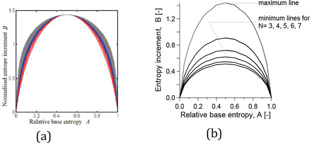
The points of the maximum B line of the entropy diagram slightly depend on N except at the symmetry point, where a = 1, A = 0.5 according to the following equation (Figure 4(a)):

Figure 4.

(a) The maximum B lines, N varies between 2 and 100. (b) the approximate minimum B lines corresponding to the 1-N-edge of the simplex.

$$A=\frac{1-a}{1-a^N}\frac{{\sum }_{i=1}^N{a}^{i-1}\left(i-1\right)}{N-1},a\ne 1$$E17

$$B=-\frac{1}{lnNln2}\left[ln\frac{1-a}{1-a^N}+ln{a}^{-\frac{a}{a-1}\frac{\left(N-1\right)a^N-{\mathit{Na}}^{N-1}+1}{\left(N-1\right)a^N-N+1}\left(N-1\right)}\right].$$E18

The points of the minimum B line of the entropy diagram are the conditional minima of B assuming the A = constant condition. These points map from the vertices and the edges of the simplex (i.e., fractions, two-fraction mixtures (Figure 4(b)). The vertices 1, 2.. N have relative base entropy coordinate A = 0, 1/(N -1), 2/(N -1)… (N -1)/ (N -1) = 1, respectively and zero B coordinate. The points of edge i – j have the following A and B coordinates:

$$A=\frac{x_i\left(i-1\right)-x_j\left(j-1\right)}{N-1}.B=-\frac{1}{lnNln2}\left[x_{i}ln{x}_i+\left(1-x_i\right)ln\left(1-x_i\right)\right].$$E19

In practice, the image of edge 1 – N is used as an approximate minimum B bounding line.

4. Properties of the entropy map

4.1 The inverse image

The inverse image of fixed A and B is the solution of the following system of equations:

$$f_1=\sum _{\mathrm{i}=1}^N{x}_i-1=0,$$E20

$$f_2=A-\frac{{\sum }_{i=1}^N{x}_i\left(i-1\right)}{N-1}=0,$$E21

$$f_3=B--\frac{1}{ln2lnN}\sum _{x_i\ne 0}{x}_{i}ln{x}_i=0.$$E22

The regular values of the entropy map are the inner points of the entropy diagram. It follows from the regular value theorem [12, 13] that the inverse image of a regular value is a manifold, these are disjunct subspaces of the simplex. For N > 2, it is an N-3 dimensional manifold, which is “circle,” situated on the A = constant, N-2 dimensional hyperplane section of the simplex, or in the isomorphic space of the grading curves (Figure 4).

The radius is determined by the difference B_max(A) - B(A). The critical values of the entropy map are the points of the maximum B line. The inverse image of a point of the maximum line of B is a single inner point of the simplex, called the optimal point, following from the concaveness of the normalized entropy increment B (Figures 5 and 6).

Figure 5.

Inverse image of fixed A, B, N = 3, 0-dimensional circles defined by 2 points. (a) in the simplex (b) in the space of grading curves.

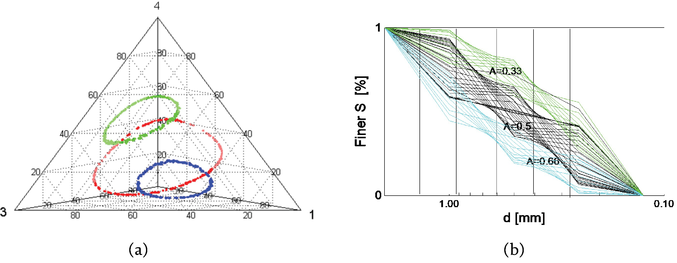
Figure 6.

Inverse image of fixed A, B, N = 4, 1-dimensional circles (a) in the simplex (b) in the space of grading curves.

The grading entropy parameter A is a linear function, the A = constant condition defines parallel hyper-plane sections of the N-1 dimensional simplex, which are related to the level lines of the A function (Figure 7). The grading entropy parameter B is a strictly concave function with a unique maximum for each A = constant value. The B = constant condition defines N-2 dimensional circles of the N-1 dimensional simplex which are related to the level lines of the B function (Figure 8).

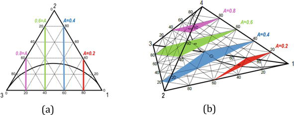
Figure 7.

Inverse image of fixed A in simplex after [10], (a) and (b) N = 3 and 4. (It can be proved that the subgraph area in the grading curves is constant for a given A value).

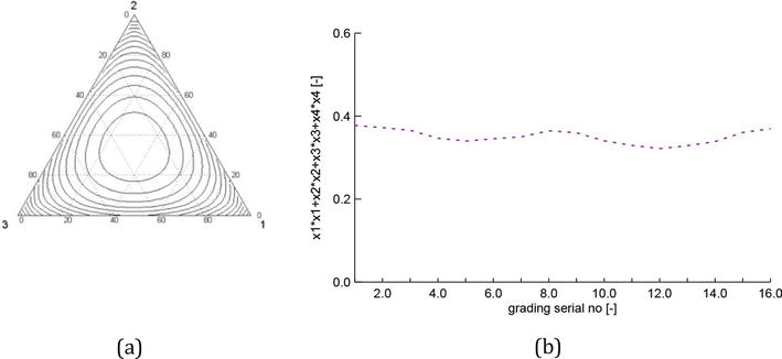
Figure 8.

(a) Inverse image of fixed B in the simplex, N = 3. (b) Sum of squared relative frequencies of the grading curves with A = 2/3, B = 1.2, N = 4 (Table 2).

4.2 Properties of the optimal grading curves

The A = constant condition defines a class of discrete distribution curves with identical subgraph area [2]. It follows from this that the optimal grading curve has a central position such that each grading curve has equal areas above and below the optimal in the same class of the gradings with A = constant.

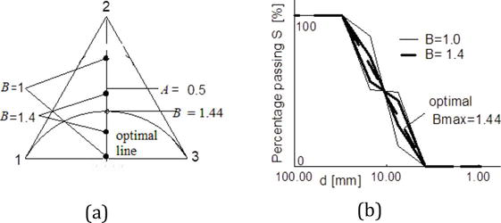
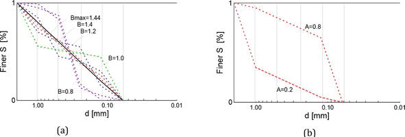
The sum of the differences (x₁ – x_1optimal) + … + (x_N – x_Noptimal) = 0 is zero, the sum of the absolute differences (denoted by delta) is related to the difference between B_max of the optimal grading curve and the B of the actual distribution in the same class (Figures 8(b) and 9(a), Table 2).

Figure 9.

(a) The mean or central position of the optimal grading curve related to fixed A = 0.5, Bmax = B = 1.44 in the class related to A = 0.5. (b) Symmetric grading curves.

	Fractal	General grading curves with A = 2/3, and B = 1.2 (some examples)
x1 [-]	0.42	0.55	0.52	0.39	0.35	0.31	0.28	0.29	0.31	0.33	0.49	0.52
x2 [-]	0.28	0.10	0.20	0.40	0.45	0.50	0.50	0.45	0.40	0.35	0.10	0.08
x3 [-]	0.18	0.14	0.05	0.03	0.05	0.08	0.17	0.23	0.27	0.30	0.32	0.28
x4 [-]	0.12	0.20	0.23	0.18	0.15	0.11	0.05	0.03	0.02	0.02	0.09	0.12
□ x1 [-]	0	0.13	0.1	−0.03	−0.07	−0.11	−0.14	−0.13	−0.11	−0.09	0.07	0.1
□ x2 [-]	0	−0.18	−0.08	0.12	0.17	0.22	0.22	0.17	0.12	0.07	−0.18	−0.2
□ x3 [-]	0	−0.03	−0.13	−0.15	−0.13	−0.1	−0.01	0.05	0.09	0.12	0.14	0.1
□ x4 [-]	0	0.08	0.11	0.06	0.03	−0.01	−0.07	−0.09	−0.1	−0.1	−0.03	0
x1^2 [-]	0.1764	0	0.2704	0.1521	0.1225	0.0961	0.0784	0.0841	0.0961	0.1089	0.2401	0.2704
x2^2 [-]	0.0784	0.01	0.04	0.16	0.2025	0.25	0.25	0.2025	0.16	0.1225	0.01	0.0064
x3^2 [-]	0.0324	0.0225	0.0025	0.0009	0.0025	0.0064	0.0289	0.0529	0.0729	0.09	0.1024	0.0784
x4^2 [-]	0.0144	0.04	0.0529	0.0324	0.0225	0.0121	0.0025	0.0009	0.0004	0.0004	0.0081	0.0144
Sum of squares i		0.30	0.38	0.37	0.35	0.35	0.36	0.36	0.34	0.33	0.32	0.36
Sum positive delta i		0.21	0.21	0.18	0.2	0.22	0.22	0.22	0.21	0.19	0.21	0.2

Table 2.

Numerical example. The A = 2/3, some grading curves with A = 2/3, and B = 1.2, positive delta is the sum of positive difference in the relative frequency with the fractal grading.

The optimal grading curves (and all grading curves) are pair-wise symmetric (Figure 9). If the same relative frequencies x_i (i = 1 … N) are used in reverse order (e.g., x’₁ = x_N, x’₂ = x_N-1 ..) then A’ = 1-A and B′ = B. Two symmetric grading curves are shown in Figure 9(b). The optimal grading curve with A and a is symmetric to the one with A’ = 1-A and a’ = 1/a, such that the same x_i (i = 1, 2, 3..N) occurs in reverse order (the symmetry for the optimal gradings appears by dividing polynomial in Eq. (16) with a^N−1).

4.3 The link of optimal and fractal grading curves

Let us examine the grading curves with N fractions and with finite fractal distribution which is described as follows [14, 15]:

$$F\left(d\right)=\frac{d^{\left(3-n\right)}-{d_{\min }}^{\left(3-n\right)}}{{d_{\max }}^{\left(3-n\right)}-{d_{\min }}^{\left(3-n\right)}}$$E23

where d is particle diameter, and n is fractal dimension. Taking into account that the fraction limits are defined by using the integer powers of the number 2, the relative frequencies of the fractions x_i (i = 1, 2, 3...N) can be expressed as follows:

$$2^{\mathrm{j}}{d}_0\ge d>2^{\mathrm{j}-1}{d}_0,$$E24

$$x_1=\frac{\left(2^{\left(3-n\right)}-1\right){d_{\min }}^{\left(3-n\right)}}{{d_{\max }}^{\left(3-n\right)}-{d_{\min }}^{\left(3-n\right)}},x_j=x_1{a}^{j-1}$$E25

$$a=2^{\left(3-n\right)},n=3-\frac{loga}{log2}$$E26

It follows that there is a one-to-one relation between the fractal dimension n and parameter a. The n varies between 3 and -∞ on the A > 0.5 side and between 3 and ∞ on the A < 0.5 side of the diagram (Figure 10), the optimal grading curves and only these have finite fractal distribution. The relation between n and A:

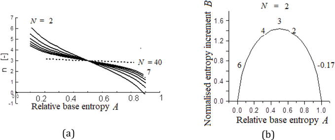
Figure 10.

(a) Fractal dimension n in terms of A and fraction number N. (b) N = 2 and 7, fractal dimension n in coordinates A = 0.1, 0.333, 0.5, 0.666, 0.9.

$$A=\frac{1-2^{3-n}}{1-2^{N\left(3-n\right)}}\frac{{\sum }_{i=1}^N\left(i-1\right)2^{\left(i-1\right)\left(3-n\right)}}{N-1},a\ne 1$$E27

The parameter a and fractal dimension n are dependent on A and N (as shown in Figure 10) except at the symmetry point of the diagram with n = 3 and a = 1 irrespective of N. Some further examples are shown in Tables 3–5 and Figure 11 which illustrates how the points related to the maximum grading entropy S may vary with N, the connecting line has a role in the internal stability.

N [−]	2	3	4	5	6	7
A [−]	0.81	0.86	0.89	0.91	0.92	0.93

Table 3.

The A coordinates for a fixed fractal dimension n = 1 (and a = 4), various N.

N [−]	2	3	4	5	6	7
n [−]	2.00	2.25	2.40	2.49	2.56	2.62

Table 4.

The fractal dimension n in the function of N at fixed A = 2/3.

N [−]	2	3	4	5	6	7	8	15	30	40
A [−]	0.67	0.71	0.76	0,79	0.82	0,84	0.86	0.93	0.97	0.97

Table 5.

The A coordinates for a fixed fractal dimension n = 2 (and a = 2), various N for the optimal point at the global maximum of the grading entropy S.

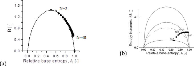
Figure 11.

The maximum grading entropy S points, N varies between 2 and 40. (a) the normalized entropy diagram. (b) Partly normalized diagram.

5. Internal stability rule

5.1 The internal stability rule for fractal soils, the probability of internal stability

The rule of the grading entropy theory [1, 16] was determined as follows. Simple vertical flow tests were designed and executed using artificial mixtures of natural sand grains. The dimensions of the permeameter were 20 cm in height and 10 cm in diameter. It was closed at the bottom by a sieve permeable of grains smaller than 1.2 mm but which retained grains larger than 1.2 mm.

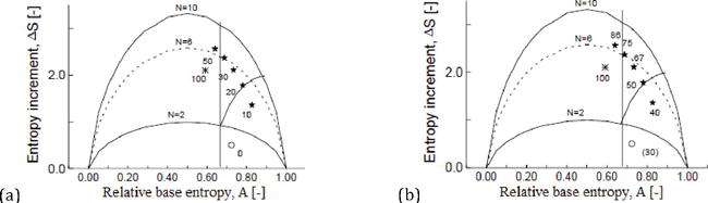
The downward hydraulic gradient i was between 4 and 5. The two parts of the permeameter were separated after the test and the grading curves were determined, the grain movement was detected from these [1]. The results of the vertical water flow (suffosion) test were represented in the partly normalized entropy diagram, in terms of the relative base entropy and the entropy increment coordinates A and ΔS, as shown in Figure 12(a).

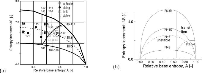
Figure 12.

Internal or grain structure stability criterion in the partly normalized diagrams. (a) Mixtures with N = 6 fractions (on the basis of [1]), with test outcome. (b) N = 6, 10, 40 fraction diagrams, simplified.

According to the results, in Zone I (if A < 2/3) piping occurs which can be interpreted such that no structure of the large grains is present, the coarse particles “float” in the matrix of the fines and become destabilized when the fines are removed by piping. This zone is separated by the 2/3 vertical line. In the Zones II and III (A = 2/3 and A < 2/3), piping cannot occur, the coarse particles gradually form a skeleton, separated by the line connecting the maximum grading entropy S points, N varies (see Figure 11).

The gap-graded grading curves with N fraction – where more than 2 fraction is missing - are found at the lower part of the diagram (indicated by letter b), below the maximum entropy increment line related to N – 2, and in this case suffusion may occur. This follows from the Terzaghi’s filter rule stating that there can be no more than two empty particle size fractions between the filter and the base soil:

$$1\le \frac{D_{\min }}{d_{\max }}\le 4$$E28

where D_min and d_max denote the diameter size of the filter and the diameter size of the base soil.

5.2 The internal stability rule for fractal soils, the probability of internally stable soils

As it was shown in Section 4.3, the fractal dimension n depends on N and A, except A = 0.5 as shown in Figure 10. Table 6 combines the internal stability rule and the fractal dimension. The fractal soil is in the stable Zone III if n < 2, independently of the value of N. The transitionally stable Zone II is between n = 2 and the n related to A = 2/3 varying in the function of N.

A [−]	N = 2	N = 4	N = 5	N = 6	N = 7
0.50	3.00	3.00	3.00	3.00	3.00
0.66	2.00	2.40	2.49	2.57	2.62
0.75	1.37	2.00	2.16	2.28	2.36
0.79	1.09	1.81	2.00	2.13	2.24
0.82	0.82	1.64	1.85	2.00	2.12
0.84	0.58	1.47	1.70	1.87	2.00

Table 6.

Fractal dimension and internal stability.

The geometrical probability of being a fractal soil expressed by the ratio of the volume of the optimal line of the simplex and the volume of the whole simplex, is trivially equal to zero. The geometrical probability of internal stability can be expressed by the ratio of the volume of the simplex of the grading curves where A > 2/3 is met and the volume of the whole simplex which tends to zero as follows.

The ratio of the volume of the simplex (ie., grading curve space) where the internal stability condition is met (A > 2/3), versus the volume of the N-1 dimensional simplex) is the geometrical probability of an arbitrary grading curve with N fractions being internally stable. This probability is decreasing with the fraction number (e.g., for N = 2, it is equal to 1/3, for N = 3, it is equal to 2/9, for N = 10, it is equal to 4/100, for N = 30, it is equal to 8/10000, see Table 7). It decreases with N (Imre – Talata [6]) while most granular soils in nature are internally at least transitionally stable.

N [−]	2	5	10	20	50
P(A > 2 /3)	3E-01	1E-01	4E-02	6E-03	2E-05

Table 7.

Geometrical probability of stability in terms of the fraction number.

6. Examples for the verification of the internal stability rule

6.1 The internal stability criterion and piping problems

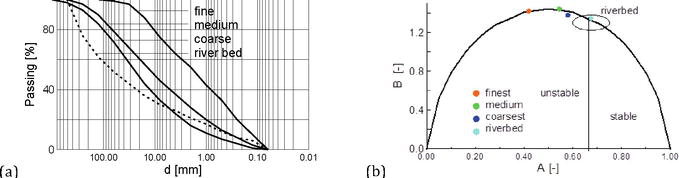
The Gouhou dam was a concrete-faced rock-fill dam 71 in high, directly founded on a sandy gravel of approximately 10 m thick [17]. The dam crest was 265 in long, and 7 m wide. The upstream and downstream slopes were 1:1.61 and 1:1.50, respectively. The damage was a piping breach. According to Figure 13(a), by the testing the rock fill materials in the grading entropy diagram for internal stability, the soils had unstable internal structures. The riverbed was not unstable alone, and all grading curves had fractal-like distribution.

Figure 13.

Piping of Gouhou dam. (a) Gradings of soil for the river bed, the finest (I), medium (II) and coarsest (III) rockfill material. (b) Gradings in the entropy diagram.

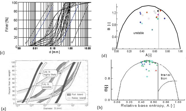
The most frequent damage in the river dyke system of Hungary is piping [18, 19]. The grading curve of the washed-out soils is silty sand and fine sand with no cohesion, with d₁₀ values within two orders of magnitude and with a small uniformity coefficient (∼C_u < 5). Both the entropy-based and classical criteria of [20, 21, 22] prove the potential for these sands to liquefy (Figure 14). According to the result of an analysis, there is a combination of static and dynamic liquefactions leading to piping here [18, 19].

Figure 14.

(a) The liquefaction criterion for washed-out soil gradings at Hungarian piping river sites. (b) the piping soils in the entropy diagram [23, 24]. (c) the liquefaction criterion by ref. [18, 20, 21, 22] for Kobe grading curves. (d) the liquefied soils in the entropy diagram (light blue: Koebe soils).

6.2 The internal stability criterion and liquefaction problems

Several seismic-induced liquefaction case studies were re-analyzed and tested for different susceptibly criteria on seismic-induced liquefaction, some results are shown in Figure 14 [23, 25]. For example, the liquefied soils in the Kobe earthquake were internally unstable, while other criteria did not indicate problematic features [20, 21, 22].

Concerning static liquefaction, some triaxial tests series were made on Houstun sand mixed with various fine contents (Figure 15, [26]) indicating that the mixtures with increasing fine content and decreasing A coordinate the static liquefaction potential increased in the transitionally stable Zone II.

Figure 15.

Static liquefaction of Houstun sand – Fine mixtures. (a) Varying fine content in %. (b) Varying static liquefaction susceptibility in % [19, 25].

7. Fragmentation and degradation paths

The natural granular soils are generally fractal, with the stable fractal dimension between 2 and 3 ([26, 27, 28, 29, 30, 31, 32, 33, 34, 35, 36, 37, 38] (Section 5.2, 6) while the probability of being fractal or internally stable is zero or tends to zero with N (Table 7). This paradox can be resolved by the directional nature of the non-normalized entropy paths and a discontinuity of the normalized entropy coordinates path during degradation of relatively young mixtures (i.e., the minimum grain size or most grain sizes are larger than the few micron-sized comminution limit, see Kendall, [39]).

During fragmentation, the non-normalized entropy path is as follows: The base entropy S₀ decreases (since the mean diameter decreases), and the entropy increment ΔS monotonically increases (Figure 16(a)) (Stabilization with lime has the opposite effect in the entropy path [40]). The discontinuity of the normalized entropy coordinates path is described theoretically and experimentally in this section.

Figure 16.

(a) Non-normalized entropy paths for the laboratory tests treated in section 7. (b) Normalized entropy path of an initially one-fraction soil with the serial number of the crushing treatment, n. legend: 1: Maximum B point. 2: Maximum S point. 3: Approximate minimum B line [4].

7.1 The theoretical entropy path at the appearance of new fractions

We assume that by definition, a possible space of the grading curves consists of such finite, discrete grain size distributions that are composed of the same N consecutive fractions with minimum grain diameter d_min. Being larger than the crushing limit.

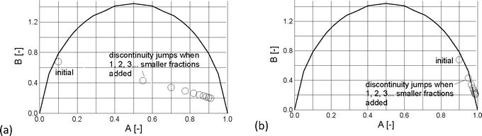
Keeping the value of N constant, the normalized and the non-normalized diagrams have the same structure, since the normalized and non-normalized coordinates are uniquely related. If we change the value of N by adding some zero fractions, the normalized coordinates of grading curve will differ (Figure 17). The difference in the case when i = 1,2 … zero fractions are added from the smaller side for a PSD:

Figure 17.

The normalized entropy diagram, representing the effect of zero smaller fractions. (a) Initially N = 2, A = 0,1. (b) Initially N = 2, A = 0.19.

$$A\left(N+i\right)-A\left(N\right)=\frac{i\left[1-A\left(N\right)\right]}{N+i-1})$$E29

$$B\left(N\right)-B\left(N+i\right)=\mathrm{\Delta }S\left(N\right)\frac{1-\frac{lnN}{lnN+i}}{lnN}$$E30

According to Figure 17, by adding 1,2..i zero fractions from the smaller side, the relative base entropy A will increase, which has some significance at fragmentation.

7.2 The entropy path in laboratory tests

The testing procedure developed to study the particle crushing phenomena was as follows [4, 5, 16]. The crushing treatments were made in a reinforced crushing pot, with the dimensions: diameter: 50 mm; height: 70 mm; wall thickness: 3 mm. Each treatment involved the application of a compressive load of 25,000 N to the sample contained in the crushing pot, using a loading machine. The sample was subjected to a series of crushing treatments (n = 1, 2 …10) then was removed from the crushing pot and the grading curve was determined by sieving. The sample was then returned.

Initially, single fraction quartz sand soil (Figure 16(b)) had an entropy path along the maximum B line, the velocity was decreasing close to the maximum entropy increment point. Theoretically it can be is important, that the fractal grading is ever present, though in case of other initial state, fractal grading would emerge later only [14, 15] as follows. Initially, two-fraction quartz and dolomitic sand mixtures with A < 0.5 [5] had a discontinuous entropy path at the start of the test due to the appearance of finer fractions, which drifted the entropy path into the stable part of the diagram (Figure 18). After the jump, a linear part entropy path occurred until the maximum entropy increment line was reached then the path followed it (Figure 18).

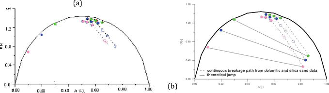
Figure 18.

Multi-compression tests with topology change and with 30 crushing treatments Trang et al. [5]. Normalized entropy path for initially N = 2 soils, every point indicates 10 crushing treatments, open symbol is quartz sand, closed symbol is dolomitic sand, the path is identical. (a) Measured data. (b) the computed jump in solid line and the subsequent path in dashed line, the entropy path is the same.

One-dimensional compression test was made with crushable grains (Light Expanded Clay Aggregate LECA) whose grains break at relatively low stress (see e.g., Casini et al. [41, 42]). The entropy path results are presented in Figure 19 showing a similar pattern as the data in Figure 18.

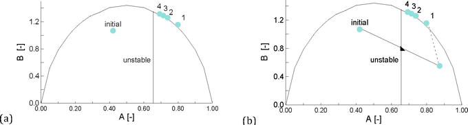
Figure 19.

Multi-compression test (Guida, parallel testing with the shear tests of Casini et al. [41, 42, 43]). (a) The normalized entropy path. (b) The computed jump in solid line the subsequent straight part in dashed line.

7.2.1 Shear - compression type laboratory tests

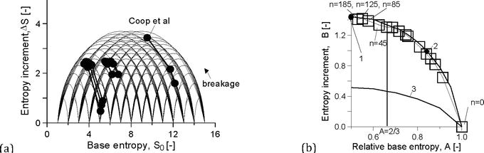
Coop et al. [43] performed a series of ring shear tests to on a carbonate sand. Two test results are shown in Figure 20(a) and Table 8. One starts from a single-fraction, with similar results as Figure 16(b). The other starts from a 3-fraction state on the A > 0.5 side of the normalized diagram, and after a jump where the A increased, a more stable final state with near fractal dimension between 2.4 and 2.8.

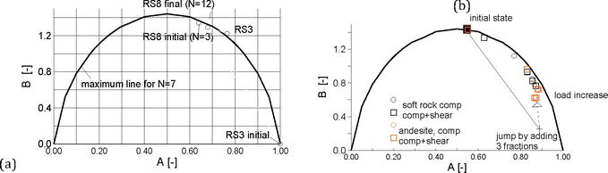
Figure 20.

Shear box test data (a) [43, 44], the initially single fraction and initially 3-fraction paths. (b) [18, 44], hard and soft rock, the computed jump in solid line the subsequent straight part in dashed line.

Sample	Rs3 (Initial grading 0,300–0,425)		Rs8 (Initial grading 0,063–0,425)
State	Initial	final	initial	final
A [−]	1	0,744	0,640	0,66,884
B [−]	0	1224	1361	12,979
S0 [−]	13	10,18	12,28	9,36
ΔS [−]	0	3042	1495	3225
n [−]	- ∞	2,62	2,37	2,76

Table 8.

Shear box test data (N final = 12) in terms of entropy coordinates and the fractal dimension n of the closest optimal point.

Dun [44, 45] performed multistage compression-shear tests on a hard rock (Andesite) and on a soft rock (Siltstone), the starting point was the same (Figure 20(b)). Twenty five samples with particle sizes ranging between 19 mm and 4.75 mm were tested. The duplicate tests seemed to have the same normalized entropy paths for the two rocks.

7.3 In situ soil compaction, in situ maturity of natural soils, soil parameters in terms of grading curve

The results of an investigation of particle disintegration of natural sandy gravel and crushed stone bedding courses due to in situ compaction and the action of construction traffic in a dozen of different sites were re-evaluated in terms of grading curves before and after compaction [46]. According to the results, when the discontinuity formula was used to estimate the normalized coordinates after compaction, assuming Weibull distribution [42, 43] and fines, the normalized entropy path differed from the case when the smalls were neglected. The results presented in Figure 21 show that with fines, the normalized parameters jumped into the transitionally stable region.

Figure 21.

Re-evaluation of compaction test results (after [46]). (a) the result of Weibull model fitting assuming 18 fractions instead of 10 fractions (resulting in about 0.06 difference in ΔS). (b) Initial and final states in the normalized diagram. Open symbol: Before, full symbol: After compaction. Circle: N = 10 and cube: N = 18 with completed fines.

An example on natural degradation is the mine rehabilitation [47], where the concept of grading entropy was applied partly to evaluate the textural evolution of waste rocks at the surface of rehabilitated mine dumps, partly to clarify the internal stability change of the soil. A series of mine-spoil samples collected from topsoils and subsoils at different periods of time.

According to the results (Figure 22), the samples showed similar trends to the soils in many fragmentation problems. The base entropy S₀ decreased (since the mean diameter decreased), and the entropy increment ΔS monotonically increased in topsoil. However, unlike fragmentation by crushing, the largest fragments were not necessarily preserved [47]. The grading curves were with near fractal dimensions between 2.5 and 2.8. The samples plotted in the transitional stability zone, the most stable is the natural sub-soil.

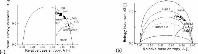
Figure 22.

Degradation of waste rock in open pit mine rehabilitation, the topsoil – Subsoil sample pairs are near fractal (the open/closed symbol: Topsoil layer/ subsoil [46]. (a) Normalized diagram (N = 17). (b) Partly normalized diagram. Topsoil is more degraded.

The use of grading entropy in assessing granular physical properties (eg., soil hydraulic conductivity, dry density, soil water retention model parameters [48, 49, 50, 51] is more and more accepted and the measurements related to the statistical relations are worthy to be made on fractal grading curves.

8. Discussion, conclusions

8.1 The entropy parameters, internal stability law

The grading entropy of a soil mixture is the statistical entropy based on uniform cells applied in terms of the log d (assuming uniform distribution within a statistical cell or on a sieve). It is the sum of two entropy coordinates: the base entropy S₀ and the entropy increment ΔS, with normalized versions (relative base entropy A, normalized entropy increment B) there are four entropy coordinates in this way.

The base entropy reflects the different sizes of the fraction cells and is a kind of mean log diameter, which is the suggested statistical variable of the grain size distribution, denoted by D. The relative base entropy A is a kind of normalized mean log diameter. Expressing the distance from the extremes (as a pseudo-metric), it has the potential to be a grain structure stability measure based on the simple physical fact that if enough large grains are present in a mixture, then these will form a stable skeleton.

The fully experimental internal stability rule of grading entropy [1] expresses that if A > =2/3, then soil is internally stable and if A < 2/3, it is internally unstable. The experimental results indicate that internal stability depends continuously on A at least in the transitional stability zone (Section 6.2). Some DEM studies prove a clear link between internal structure and internal stability, the mechanical coordination number [2] was increasing in terms of A.

8.2 Soil classification on the basis of internal stability, mean grading curves

The normalized grading entropy coordinates – due to their such physical meaning that they express internal stability – may classify well the grading curves with N fractions. The grading curves with fixed A is a class with fixed internal stability, and the grading curves with fixed coordinate pair A and B is a disjunct subclass.

Each class has a unique optimal grading curve with maximum entropy increment, which is a fractal grading curve and a mean grading curve for the given class in the following sense. Every grading curve in the class has an equal subgraph area and deviates from the mean grading curve that equal areas are found above and below the mean grading curve, the difference is dependent on the B coordinate.

The optimal grading curves have a finite fractal distribution. The optimal or fractal grading curves have fractal dimensions between minus to plus infinity. The fractal soil is in the stable Zone III if n < 2, independently of the value of N. The transitionally stable Zone II is between n = 2 and the n related to A = 2/3 varying in the function of N.

The natural granular soils are generally fractal, with the stable fractal dimension between 2 and 3 [26, 27, 28, 29, 30, 31, 32, 33, 34, 35, 36, 37, 38] verifying the internal stability rule of grading entropy.

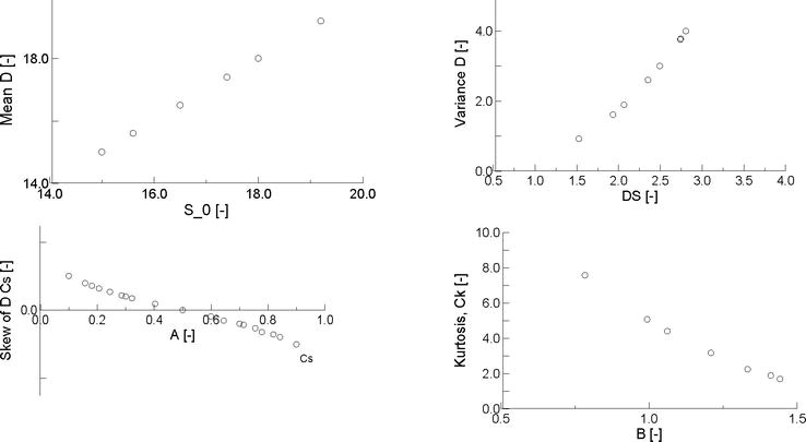
The mean functions constructed from simulated mean or fractal grading curves ([3], Figure 23) showed that entropy coordinates are similar to the four central moments as follows: The base entropy S₀ is identical to the first central moment and the entropy increment ΔS is similar to the variance, both are dependent on N. The relative base entropy A and the normalized entropy increment B are in one-to-one, smooth relation with the skew and the kurtosis, respectively, basically independently of N.

Figure 23.

Numerical experiment on the data of a series of mean, finite, discrete distribution functions with N = 7 statistical cells. (a) To (d): The relationships of the first four central moments in terms of the abstract diameter D [−] and the four entropy coordinates.

The entropy increment is better for the description of the dispersion than variance (i.e., second central moment) for gap-graded [46] and bimodal mixtures (see the Appendix). It measures how much the N fractions influence the soil behavior.

8.3 The entropy path and degradation

The space of the grading curves is isomorphic to an N-1 dimensional simplex, which is the continuous sub-simplex of a larger dimensional simplex. The grading entropy coordinates are smooth function on this simplex, the image of one base entropy and one entropy increment coordinates is called as entropy diagram. Every grading curve plot as a point in the diagram, a degradation process is a path in the diagram.

The natural granular soils are generally fractal, with a fractal dimension between 2 and 3 [26, 27, 28, 29, 30, 31, 32, 33, 34, 35, 36, 37, 38]. Since natural soils are generally within this fractal dimension bounds, the internal stability rule is verified by the nature. However, the probability of being fractal or internally stable is zero or tends to zero with N (Table 7). This paradox can be resolved by two features of the normalized entropy paths, the directional nature and a discontinuity feature of the degradation path.

During fragmentation, the non-normalized entropy path is the same, the base entropy S₀ decreases (since the mean diameter decreases), and the entropy increment ΔS monotonically increases (Figure 16(a)). (Stabilization with lime has the opposite effect in the entropy path [40]).

The fact that the space of the grading curves is isomorphic to an N-1 dimensional simplex, can be used to compute the geometrical probability that an accidental grading curve is fractal or internally stable which is zero and near zero decreasing with the fraction number N [6], respectively. This paradox that natural soils are mostly fractal and internally stable can be explained by the degradation process which is directional and the related non-normalized entropy path contains some discontinuity at the appearance of small fractions drifting the path into the stable domain as follows.

The extension of the grading entropy map onto a larger simplex is technically possible, by completing the original grading curves with zero fractions. The extended map is continuous for the non-normalized coordinates and has a discontinuity for the normalized coordinates. This fact has a practical significance since in nature the degradation results in some new fractions (the N increases), and the internal stability rule is formulated in terms of normalized or relative base entropy A which changes if N increases.

However, by changing the fraction number N, in the case of appearing some smaller fractions, a discontinuity occurs which can be computed. The computed path is a drift toward the more stable region. Then, after the discontinuity, the normalized entropy path under a constant fraction number is as follows. The relative base entropy A decreases and the normalized entropy increment B monotonically increases, until the maximum normalized entropy increment line is reached along a linear path. Then the path proceeds along it, through various fractal distributions with decreasing rates toward the symmetry points of the diagram. The path seems to be independent of the material, which may serve as a basis of some rock qualification or compaction control tests.

Acknowledgments

Thanks for the communications on particle breakage with Professor Itai Einav. The help of the Laboratories of the Department of Engineering Geology BME in the testing is acknowledged. This publication contains the work of PhD Student Phong Quoc Trang. Thanks for the contribution of dr. István Talata, dr. James Leak, dr. Daniel Barreto.

A. Historical background (some pieces)

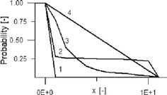
The Shannon entropy was first used for soils by Harrop-Williams, 1983 [52] using d as a statistical variable instead of log d. By a numerical example on gap-graded grading curves, the entropy was found to be better for the dispersion than variance. There is an example in Figure A1 and Table A1. The variance is a maximum of the gap-graded grading curve, it is not maximal in terms of entropy, the gap-graded grading curves with N fractions plot below the N-2 maximum entropy increment line (see Figure 12(a).

Figure A1.

Various distributions.

	distribution	1	2	3	4
mean	1	3.49	2.91	6
variance	0	17.83	4.76	10
entropy	0	1220	2559	3459

Table A1.

Mean, variance and entropy increment of distributions on 11 cells, varying from 1 to 11.

Lőrincz [1] elaborated the full theory, the relation with dry density and made the experiences for the grading entropy based rules. For the d₀, for the elementary cell width (Table 1), the height of the SiO₄ tetrahedron was suggested by Imre et al. (d₀ = 2⁻²² mm [9, 53]). The first DEM applications were made eg. in [2], the first applications of the rules were made eg., by [9, 20, 25, 46, 52, 53].

The finite fractal distribution (by mass) formula was derived by Einav [14, 15]. The identity of the optimal grading curves of grading entropy (defined by Lőrincz [1]) and the finite fractal grading curves was revealed by Imre (published in Imre-Talata [6]). It was shown that the relations of the mean grading curves are mean relations (Imre et al. [3]).

Talata [40] revealed that the probability of internally stable mixtures decreases with N (Imre-Talata [6]). By using the simplex analogy [2], the probability of fractal mixtures is zero. In nature, the fractal gradings with fractal dimension 2 to 3 are very frequent (Section 6, [27, 28, 29, 30, 31, 32, 33, 34, 35, 36, 37, 38, 39]). The paradox is solved by the normalized grading entropy path [6]. The breakage process was related to grading entropy first by [1, 5]. The interpolation of model parameters in terms of the grading curve started by e.g., [1, 54, 55, 56].

List of notations

A	relative base entropy
B	normalized entropy increment
CU	uniformity coefficient given by the following expression d60/d10.
dh	harmonic mean diameter
d10	diameter of which 10% of the particles are finer
d60	diameter of which 60% of the particles are finer
Ss	statistical entropy
S0	base entropy
ΔS	entropy increment
M	Number of elements in statistical cell
Mi	Number of elements in the ith cell
m	Number of equivalent cells
s	Specific entropy
α	Frequency of elementary cells elements in the sieve cell
S	Total grading entropy
x	Relative frequency of PSD
N	is the number of fractions

References

1.Lőrincz J. Grading Entropy of Soils Doctoral Thesis. BME, Budapest (in Hungarian): Techn Sciences; 1986
2.Imre E, Talata I, Barreto D, Datcheva M, Baille W, Georgiev I, et al. Some notes on granular mixtures with finite, discrete fractal distribution. Periodica Polytechnica. Civil Engineering. 2022;66(1):179-192
3.Imre E, Hortobágyi ZS, Illés ZS, Nagy L, Talata I, Barreto D, et al. Statistical parameters and grading curves. In: Proceedings of the 20th International Conference on Soil Mechanics and Geotechnical Engineering. (20th ICSMGE). Sydney: Australian Geomechanics Society; 2022. pp. 713-718
4.Lõrincz J, Imre E, Gálos M, Trang QP, Rajkai K, Fityus S, et al. Grading entropy variation due to soil crushing. International Journal of Geomechanics. 2005;5(4):311-319
5.Trang PQ, Kárpáti L, Nyári I, Szendefy J, Imre E, L?rincz J. Entropy concept to explain particle breakage and soil improvement. In: Proc of the Young Geo Eng Conf. Alexandria, Egypt; 2009. pp. 87-90
6.Imre E, Talata I. Some comments on fractal distributions and the grading entropy theory. In: Proceedings of the MAFIOK. Budapest: Szent István University; 2017. pp. 123-130
7.Korn GA, Korn TM. Mathematical Handbook for Scientists and Engineers: Definitions, Theorems, and Formulas for Reference and Review. Courier Corporation; 2000
8.Imre E. Characterization of dispersive and piping soils. In: Proceedings of the European Conference on Soil Mechanics and Foundation Engineering. (XI. ECSMFE), Copenhagen, 1995. 2. 49-55
9.Imre E, Lõrincz J, Rózsa P. Characterization of some sand mixtures. In: Proc. of 12th IACMAG; October 2008. Goa, India; 2008. pp. 2064-2075
10.Singh VP. Entropy Theory in Hydraulic Engineering: An Introduction. American Society of Civil Engineers. ASCE; 2014. p. 656
11.Imre E, Kabey D. An extension of Thales' theorem-based geometric interpretation of the arithmetic-geometric means. Eng. Symposium in Bánki. 2022. pp. 157-163. Available from: https://bgk.uni-obuda.hu/esb/in_Hungarian.
12.Milnor J, Weaver DW. Topology from the Differentiable Viewpoint. Princeton university press; 1997
13.Hirsch MW. Differential Topology. Graduate Texts in Mathematics 1973 GTM, Volume 33 Hardcover ISBN: 978–0–387–90148-0 Copyright Information. New York: Springer-Verlag
14.Einav I. Breakage mechanics—Part I: Theory. Journal of the Mechanics and Physics of Solids. 2007;55(6):1274-1297
15.Einav I. Breakage mechanics—Part II: Modelling granular materials. Journal of the Mechanics and Physics of Solids. 2007;55(6):1298-1320
16.Lőrincz J, Imre E, Fityus S, Trang PQ, Tarnai T, Talata I, et al. The grading entropy-based criteria for structural stability of granular materials and filters. Entropy. 2015;17(5):2781-2811. 31 p
17.Zhang LM, Chen Q. Seepage failure mechanism of the Gouhou rockfill dam during reservoir water infiltration. Soils and Foundations. 2006;46(5):557-568
18.Tsuchida H. Prediction and counter measure against the liquefaction. Seminar in the Port and Harbor Research Institution. 1970;3(1-3):33
19.Rahemi N. Evaluation of Liquefaction Behavior of Sandy Soils Using Critical State Soil Mechanics and Instability Concept. PhD Thesis. Civil and Environmental Engineering Ruhr-University Bochum; 2017
20.Barreto, Gonzalez D, Leak J, Dimitriadi V, McDougall J, Imre E, et al. Grading entropy coordinates and criteria for evaluation of liquefaction potential. In: Proceedings of the 7th International Conference on Earthquake Geotechnical Engineering. London: CRC Press; 2019. pp. 1346-1353
21.Ishihara K. Terzaghi oration: Geotechnical aspects of 1995 Kobe earthquake. 1999. 14th ICSMFE
22.Numata A, Mori S. Limits in the gradation curves of liquefiable soils. In: World Conf Earthquake Eng Vancouver, No. 1190. 2004
23.Nagy L. The grading entropy of piping soils, Zbornik Radova Gradevinskog Fakukteta 20. In: Universitet u Novum Sadu Gradevinski Fakultet. Subotica; 2011. pp. 33-46. ISSN 0352-6852
24.Imre E, Lorincz J, Trang PQ, Barreto D, Goudarzy M, Rahemi N, et al. A note on seismic induced liquefaction. In: XVII ECSMGE - Reykjavík, Iceland 1–6 of Sept 2019. IGS; 2019. pp. 979-988
25.Imre E, Nagy L, Lorincz J, Rahemi N, Schanz T, Singh VP, et al. Some comments on the entropy-based criteria for piping. Entropy. 2015;17(4):2281-2303. 23 p
26.Palmer AC, Sanderson TJO. Fractal crushing of ice and brittle solids. Proceedings of the Royal Society of London. Series A, Mathematical and Physical Sciences. 1991;433(1889):469-477
27.Steacy SJ, Sammis CG. An automaton for fractal patterns of fragmentation. Nature. 1991;353:250-252
28.Roberts JE, de Souza JM. The compressibility of sands. Proceedings of ASTM. 1958;58:1269-1277
29.Hagerty MM, Hite DR, Ulrich CR, Hagerty DJ. One-dimensional high-pressure compression of granular material. Journal of Geotechnical Engineering. 1991;119(1):1-18
30.Okada Y, Sassa K, Fukuoka H. Excess pore pressure and grain crushing of sands by means of undrained and naturally drained ring-shear tests. Engineering in Geology. 2004;75(3–4):325-334
31.Sadrekarimi A, Olson SM. Particle damage observed in ring shear tests on sands. Canadian Geotechnical Journal. 2010;47(5):497-515
32.Ho TYK, Jardine RJ, Anh-Minh N. Large displacement interface shear between steel and granular media. Geotechnique. 2011;61(3):221-234
33.Pál G, Jánosi Z, Kun F, Main IG. Fragmentation and shear band formation by slow compression of brittle porous media. Physical Review E. 2016;94:053003
34.Kun F. Breakage of particles, session introduction. In: P&G Conference, Montpellier, 2017. 2017
35.Sammis CG, King G, Biegel R. Kinematics of gouge deformations pure. Applied Geophysics. 1987;125:777-812
36.Airey DW, Kelly RB. Interface Behaviours from Large Diameter Ring Shear Tests Proceedings of the Research Symposium on the Characterization and Behaviour of Interfaces. Atlanta, GA, USA; 2008. pp. 1-6
37.Imre B, Laue J, Springman SM. Fractal fragmentation of rocks within sturzstroms: Insight derived from physical experiments within the ETH geotechnical drum centrifuge. Granular Matter. 2010;12(3):267-285
38.McDowell GR, Bolton MD, Robertson D. The fractal crushing of granular materials. Journal of the Mechanics and Physics of Solids. 1996;44(12):2079-2101
39.Kendall K. The impossibility of comminuting small particles by compression. Nature. 1978;272(5655):710-711
40.Harrop-Williams K. Some geotechnical applications of entropy. In: Proc. of the 4th ICASP. Vol. 2. 1983
41.Casini F, Giulia M, Viggiani B, Springman SM. Breakage of an artificial crushable material under loading. Granular Matter. 2013;15:661-673. DOI: 10.1007/s10035-013-0432
42.Guida G, Bartoli M, Casini F, Viggiani GMB. Weibull distribution to describe grading evolution of materials with crushable grains. Procedia Engineering. 2016;158:75-80
43.Coop MR, Sorensen KK, Bodas Freitas KK, Georgoutsos G. Particle breakage during shearing of a carbonate sand. Geotechnique. 2004;54(3):157-163
44.Dun R. The Importance of Particle Breakage for Shear Strength Measured in Direct Shear. Undergraduate honours thesis. The School of Engineering. The University of Newcastle (unpublished); 2014
45.Fityus S, Imre E. The significance of relative density for particle damage in loaded and sheared gravels powders and grains 2017. In: 8th International Conference on Micromechanics on Granular Media. 2017. DOI: 10.1051/epjconf/201714007011. 4 p
46.Imre E, Lõrincz J, Trang PQ, Casini F, Guida G, Fityus S, et al. Reanalysis of some in situ compaction test results. In: Proc of the XVII ECSMGE-2019. Reykjavík; 2019. Paper: 0989. DOI: 10.32075/17ECSMGE-2019-0989
47.Imre E, Fityus S. The use of soil grading entropy as a measure of soil texture maturity and internal stability. In: Proceedings of the (XVI. DECGE). Macedonia; 2018. pp. 639-644
48.Feng S, Vardanega PJ, Ibraim E, Widyatmoko I, Ojum C. Permeability assessment of some granular mixtures. Géotechnique. 2019;69(7):646-654. DOI: 10.1680/jgeot.17.T.039
49.O’Kelly BC, Nogal M. Determination of soil permeability coefficient following an updated grading entropy method. Geotechnical Research. 2020;7(1):58-70, 13 p. DOI: 10.5772/intechopen.69167
50.Imre E, Firgi T, Baille W, Datcheva M, Barreto D, Feng S, et al. Soil parameters in terms of entropy coordinates. In: E3S Web of Conference. Vol. 382. UNSAT; 2023. p. 25003. DOI: 10.1051/e3sconf/202338225003
51.Imre E, Barreto D, Datcheva M, Singh VP, Baille W, Feng S, et al. Minimum dry density in terms of grading entropy coordinates. In: Proceedings of the 17th Asian Regional Conference on Soil Mechanics and Geotechnical Engineering; 14-18 August 2023; 17th ARC, Astana, Kazakhstan. London, UK: CRC Press; 2023. pp. 402-406, 5 p. DOI: 10.1201/9781003299127-42
52.Imre E, Lörincz J, Szendefy J, Trang PQ, Nagy L, Singh VP, et al. Case studies and benchmark examples for the use of grading entropy in Geotechnics. Entropy. 2012;14:1079-1102
53.Talata I. A volume formula for medial sections of simplices. Discrete & Computational Geometry. 2003;30:343-353. DOI: 10.1007/s00454-003-0015-6
54.Imre E, Lőrincz J, Trang QP, Fityus S, Pusztai J, Telekes G, et al. A general dry density law for sands. KSCE Journal of Civil Engineering. 2009;13(4):257-272
55.Imre E, Rajkai K, Genovese E, Fityus S. The SWCC transfer functions of sands. In: Proceedings of 4th Asia-Pacific Conference on Unsaturated Soils. 2009. pp. 791-797, 7 p
56.Imre E, Rajkai K, Genovese E, Jommi K. A SWCC transfer functions of sands. In: Proc. of 5th Int. Conf. on Unsaturated Soils. 2010. pp. 453-459, 7 p
Written By
Emőke Imre and Vijay Pal Singh
Submitted: 29 August 2023Reviewed: 18 September 2023Published: 08 April 2024
Open access peer-reviewed chapter