Computer Simulation of Mechanisms to Reduce the Metabolic Costs of Running While Taking into Account the Individual Characteristics of the Athlete

Abstract

Previous research demonstrates the relationship between the biomechanical characteristics of running and running economics (RE). An increase in results in cycle-based sports is connected with the improvement of motion biomechanics tailored for individual athletes. The purpose of the chapter is to conduct a computer simulation of the use of biomechanical mechanisms of the lower limb muscles during running, leading to a decrease in metabolic costs. Eight biathletes took part in the experiments: all from the top 30 world ratings at the time of the study. For experiments, we used a Qualisys motion capture system, a power plate (Tredmetrix) mounted on a treadmill, a Biodex-3 complex, and a Metamax-3 gas analyzer (Cortex). OpenSim software allows modeling based on collected experimental data. This study describes the methodology of an individual approach to the process of training elite-level athletes based on computer modeling. In particular, we studied the possibility of reducing metabolic costs when working above the anaerobic limit, that is, similar to the actual competitive speed for biathlon and cross-country skiing. The results of the model experiment clearly demonstrated that one of the potential ways to reduce metabolic costs during running is the individualization of the use of biomechanical mechanisms for performing repulsion in a running step.

1. Introduction

Constant improvement in achievements in sport drives the necessity to search for new ways of increasing efficiency. There are on-going discussions on how to improve the way the world’s top athletes perform in cyclic sports, including athletic running.

Running economy (RE) is typically defined as the amount of energy used to run at a certain speed without reaching maximum capacity. It is measured by observing the oxygen consumption and the Respiratory Exchange Ratio in a steady-state.

It is becoming increasingly clear that aerobic capacity training is not the only means of improving endurance performance [1]. The performed study demonstrates the relationship between the biomechanical characteristics of a run and its RE [2, 3, 4, 5, 6]. An increase in results in cycle-based sports is connected with the improvement of motion biomechanics tailored for individual athletes.

First of all, the training process personalization (or individualization) is based on understanding and using athlete’s individual technique for performing the “main competitive exercise”—in our case, it is running. The individual technique is largely dependent on the architectonics of athlete’s muscle groups and their interaction during motion.

Many researchers emphasize on the connection between lowering the energy consumption for COM (Center of Mass) movement and lowering the metabolic cost of muscles in lower limbs [7, 8, 9, 10]. Another important mechanism that allows lowering the running metabolic cost is the use of elastic-viscous properties of muscles and the ability to store the elastic strain energy (ESE) in specific cases [11, 12, 13, 14].

The analysis of elite-level athletes’ movement specialties is possible by using an individual approach. The athletes have very different anthropometry and physical abilities (including force characteristics). Each sportsman has his/her own style of movement based on years and years of training. The research question should provide recommendations for a specific athlete, as it is almost near to impossible experimentally study the differences between elite-level athletes. This is largely due to the lack of option to have a statistically controlled environment: well performing athletes and those who are not doing well, different classification groups of athletes, the impact of different training methods used by different groups, etc.

But to some extent, these questions can be answered using individual computer modeling. In this case, the search for the most efficient “style” or technique is performed using multiple simulations on the same model with different control parameters that affect the end result.

OpenSim software [15] allows running simulation based on experimental (recorded) data and modeling the change of the running style while changing key influencing factors for the selected athlete. As a result, there is a way to quantify and analyze the differences in various running options for a specific athlete.

The purpose of the chapter is to conduct a computer simulation of the use of biomechanical mechanisms of the lower limb muscles during running, leading to a decrease in metabolic costs. It is assumed that a decrease in metabolic costs can occur due to the optimization of muscle activity over time.

This study is aimed to provide usable results which can be embedded in the training process of professional athletes. Most training programs for sportsmen include strength exercises, but for top level athletes these need to be proven effective given their individual features and characteristics. The results of this research allow the development of individual training plans, including force-based training aimed at specific muscle groups in order to “correct” the running style for lower energy consumption.

2. Methods

To solve the goal set in the work, eight male athletes were selected from the athletes of the national teams of Russia in biathlon (age 25 ± 3.4 years; height 1.82 ± 3.8; weight (76 ± 4.1 kg). The athletes are in the top-30 of world ratings at the moment of the study.

To control the training process in the biathlon national teams of Russia, athletes are tested before each stage of sports training. Testing involves running a test with incremental velocity to determine the aerobic and anaerobic limits of the studied athletes, as well as estimating the maximal oxygen consumption VO₂max metric using Metamax-3 (Cortex, Germany) gas analyzer system. The recorded parameters were used to calculate the rates of O₂ consumption and CO₂ excretion, respiratory quotient, ventilation equivalents of O₂ consumption and CO₂ excretion. These indicators were calculated automatically by the program included in the “Metamax-3”. The same program was used to determine the level of the anaerobic threshold using the V-slope method [16].

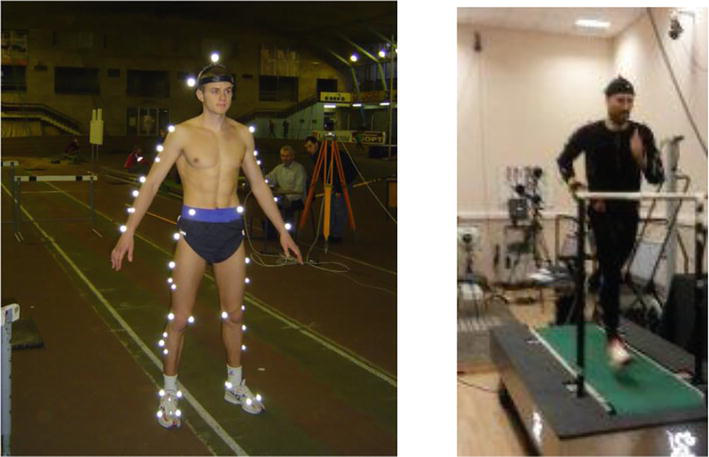
For the experimental part of the study we used a motion capture system involving 18 high-speed Oqus 3+ cameras (Qualisys, Sweden)) with the frame rate of 400 frames per second. The running exercise was performed on a treadmill-mounted force plate (Tredmetrix, USA). The data obtained from the force platform made it possible to obtain indicators of the longitudinal and vertical reaction of the ground reaction, as a resultant vector, as well as the coordinates of its application [13]. Cameras and force plate sensors were synchronized using a specific adapter. A total of 54 reflecting markers (1 cm in diameter) were mounted on the study subjects according to Figure 1. Athletes were also tested using force-study complex Biodex 3 (Biodex, USA). The strength indicators (peak torque) of athletes were assessed during flexion-extension of the knee joint in the isokinetic mode at low speed (60 deg./s) according to the method [17]. In this study, subjects were running at speeds of 3 m/s and 5.1 m/s, respectively. The sequence of testing athletes was carried out as follows. After a standard warm-up lasting 5–8 minutes, the athletes tested their strength capabilities. Flexion-extension test in the knee joint was performed five times with each leg for each movement, in accordance. After that, 8–10 minutes were allotted for attaching markers to the body of athletes for shooting and a gas analyzer. Then the athlete performed a warm-up run at an arbitrary speed for 3–5 minutes on the treadmill. When ready, the athlete ran at a speed of 3 m/s. After the athlete reached his individual aerobic threshold, kinetic and kinematic data were recorded for 10 s. Subsequently, the speed of the treadmill increased to 5.1 m/s. After 10 s after obtaining the values of the anaerobic threshold according to the gas analyzer “Metamax-3”, kinetic and kinematic data were recorded for 10 s.

Figure 1.

Placement of the markers on the subject and the procedure for carrying out the test.

With respect to the first method of increasing repulsive power, it is known that the pre-stretch of the muscle-tendon complex (MTC) enhances its subsequent contraction. It is manifested in various locomotions [11, 18, 19, 20]. Thus, they can increase or decrease muscle stiffness [14, 21, 22, 23]. Accordingly, it becomes possible to use the mechanism of elastic deformation in the muscles. Such a mechanism is sometimes called a “catapult” [24].

The second way to increase the power of a take-off is based on energy transfer through biarticular muscles. This process involves processes which occur in the musculotendinous unit (MTU) and is supported by the fact that the powerful monoarticular gluteus muscles, mainly the gluteus maximus (GM), play a significant role in hip extension, thus increasing hip joint angle. The energy transfer from GM to the knee joint occurs via the biarticular RF muscle. This muscle produces the greatest power output when contracting slowly and working in nearly isometric conditions. Additionally, the knee joint is extended by RF and a collection of monoarticular m.vastus (VA) muscles [25]. The triceps muscle of the calf is the primary muscle involved in this movement. It works in conjunction with the gastrocnemius muscle (GA) to transfer energy and create a reinforcing contraction. This is known as the “Energy Transfer Model” and is described in detail in the study “Knee Extension and Plantar Flexion: Energy Transfer Model” [19].

Athletes were divided into two groups in accordance with the use of two different mechanisms of muscle work during repulsion in a running step. Athletes’ data and parameters can be found in Table 1.

Group	Height, m	Weight, kg	VO2 max	Strength of knee flexion in the isokinetic mode with 60 degrees/s/kg
Group A (n = 4)	1.83 ± 3.4	82.3 ± 2.1	71.9 ± 4.3	2.7 ± 0.8
Group B (n = 4)	1.81 ± 4.1	71.7 ± 1.8	74.6 ± 3.5	2.0 ± 0.6

Table 1.

Key characteristics of studied athletes.

According to available studies, it is assumed that an athlete uses only one type of mechanism in different locomotion [13, 14], which determines the individuality of the technique for performing competitive exercises.

2.1 Data processing approach

Kinematic and dynamic calculations were conducted using the full-body model proposed in the Hamner and Delp paper [1]. This simulation enabled a deeper understanding of the body’s behavior with regards to the kinematic and dynamic calculations, and provided a more comprehensive evaluation of the motion. We used a three-dimensional musculoskeletal model with 29 degrees of freedom, 92 lower extremity and torso muscles, and arms driven by torque actuators, which has been used previously to study how each muscle contributes to accelerating the body’s center of mass during running [1, 26]. In order to perform the analysis of metabolic costs during the running experiment a group of key muscles was selected: PSO (psoas), GMAX (superior, middle, and inferior gluteus maximus), BF (biceps femoris long head), SEM (semimembranosus and semitendinosus), RF (rectus femoris), VAS (vastus medialis), GAS (lateral compartments of gastrocnemius), SOL (soleus) and TIB (tibialis anterior). We first simulated five running cycles for each subject at each speed, following the methods described by Hamner and Delp [1]. The running cycle has two phases: the stance, or support phase and the flight phase (transfer of the fly leg). The stance phase is the push of the foot, the first contact of the foot with the ground. The beginning and end of the support phase in the running cycle was carried out according to the appearance and disappearance, respectively, of the vertical force according to the power platforms of the treadmill verification of the model we built for each athlete was carried out by comparison with identical models of athletes [1] located in the repository https://github.com/modenaxe/awesome-biomechanics#running-running

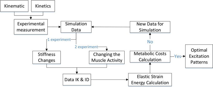
The flow chart of the organization of research and model experiments is presented in Figure 2. Our process of simulation started by adjusting the measurements of the generic musculoskeletal model to fit the body proportions of each of our subjects, accomplished by using the OpenSim Scale Tool. Additionally, we also modified the maximal isometric strength of the muscles by using a regression equation based on the mass and height of each subject [27].

Figure 2.

Flow chart summarizing computational and experimental approaches for evaluating the energetics of locomotion.

In order to calculate the joint angles at each time in the model, the “inverse kinematics” tool in OpenSim was used. The marker locations on the model were then optimized to match the trajectories of the corresponding markers measured on the subject, so the sum of the squared distances between the two marker sets was minimized, resulting in the optimal set of joint kinematics. The “inverse dynamics” tool in OpenSim was used to determine the net joint moments. The ground reaction forces were applied to the feet of the model, and the equations of motion were solved to calculate the joint moments. The “static optimization” tool in OpenSim was then used to calculate the net joint moments. This procedure was used to solve a minimization problem, the aim of which was to reduce the sum of the squares of all muscle activations, that is, to reduce total muscle stress. Constraints were applied to the optimization solution, which needed to fit the force-length-velocity surface of each muscle.

Each muscle produces mechanical power by multiplying the musculotendon force and the musculotendon velocity. The mechanical work is found by calculating the area beneath the power-time curve. Concentric contractions signify the energy generated by the muscle (positive work), while eccentric contractions represent the energy consumed (negative work).

The quantification of lower-limb muscle function was accomplished by computing each muscle’s contribution to the ground reaction force and lower-limb joint accelerations derived from the experiment. This was achieved using the “pseudo-inverse induced acceleration analysis” and a custom plugin from OpenSim (available at https://simtk.org/home/tims_plugins).

The isolated muscle force was applied to the model one at a time. This force was then transmitted to all of the body segments, causing: (1) a ground reaction force at the foot; and (2) angular accelerations in all body joints. This technique for computing the muscle’s contributions to ground reaction forces and lower-limb joint accelerations has already been validated using running data .

We used OpenSim’s Computed Muscle Control (CMC) Tool [28] to generate muscle-driven motions based on the recorded experiments, with the single adjusted model and the adjusted kinematics. CMC calculates the muscle stimulation required to generate the perceived running motion, while decreasing the total of squared muscle activations at standard intervals in the motion. Precisely, the objective function J of CMC consists of an effort term J_effort and a term associated with modeling and measurement mistake J_error:

$$J=J_{\text{effort}}+J_{\text{error}},$$E1

$$J_{\text{effort}}=\sum _{i\in M}{a}_i^2,$$E2

$$J_{\text{error}}=\sum _{i\in R}{\left(\frac{f_i}{w_{f,i}}\right)}^2.$$E3

The effort term (Eq. (2)) depends only on the activation of the corresponding muscle group. Eq. (3) penalizes the force or moment f delivered by the set of reserve and residual actuators R, in accordance with [28]. Reserve actuators supply minor joint moments to make up for unmodeled passive structures (such as ligaments) and potential muscle weakness, while residual actuators apply any residual forces. The weighting factor w_f,i is adjusted to make the reserves and residuals much more expensive to use in comparison to the muscles; in OpenSim, this factor is referred to as the actuators’ optimal force property.

2.2 Elastic strain energy (ESE) calculation

During the analysis we attempted to calculate the possible amount of storing and utilizing the elastic strain energy (ESE) according to the methodology suggested by Prilutsky et al. [13, 14].

Mechanical energy can be transferred between the joints of the leg in five main ways (Table 2).

No.	Pj(t)*	Pj^c(t)	∑jP^m(t)	The rate and direction of energy transmission through the two-joint muscles	The roles of the muscles that serve the jth joint
1	>0	>0	≥0	To the jth joint at a rate of ⸡Pj(t)⸠ from the side of the (j − l)th and/or (j + I)th joints	Generate energy at a rate of ⸠Pj^c(t)⸠ − ⸠Pj(t)⸠
2	<0	≥0	>0	From the jth joint at a rate of -Pj(t)⸠ to the (j − 1)th and/or (j + 1)th joints	Generate energy at a rate of ⸠Pj^c(t)⸠ + ⸠Pj(t)⸠
3	>0	≤0	<0	To the jth joint at a rate of ⸡Pj(t)⸠ from the side of the (j − 1)th and/or (j + 1)th joints	Absorb energy at a rate of -[⸠Pj^c(t)⸠ + ⸠Pj(t)⸠]
4	<0	<0	≤0	From the jth joint at a rate of ⸺⸡Pj(t)⸠to the Cj − 1)th and/or (j + 1)th joints	Absorb energy at a rate of -[⸠Pj^c(t)⸠- ⸠Pj(t)⸠]
5	=0	≥0, <0	≥0, <0	(a) Energy is not transferred through two-joint muscles. (b) Energy is delivered to the jth joint at a rate of ⸠Pj(t)⸠ [e.g., from the side of the (j + 1)th joint] and transferred from it at a rate of -⸠Pj(t)⸠ [e.g., to the (j − l)th joint]	Generate energy at a rate of ⸠Pj^c(t)⸠ or absorb energy at a rate of -⸠Pj(t)⸠

Table 2.

Variations of mechanical energy exchange between the two-joint muscles [13].

^*

At any given time t, Pj(t) is the energy transferred between two-joint muscles at the jth joint. The power developed by the joint moment at the jth joint is P_j^c(t), while ∑_jP^m(t) is the sum of the powers developed by all the muscles serving the jth joint.

Five major pathways for energy transfer are listed in Table 2 [13].

2.3 Metabolic costs calculation

To evaluate metabolic energy consumption from the simulations, we used a modified version of the metabolic model developed by Umberger et al. [29] and Verkhoshansky and Verkhoshansky [30]. This model was implemented in OpenSim v3.3 using the Umberger2010MuscleMetabolicsProbe.

In accordance with the calculation method, we added up the energy consumption rate of all muscles, as well as a basal rate (1.2 W/kg) [31], then incorporated the total rate in the running cycle and divided by the length of time the athlete’s supporting leg was on the support. This process was used to estimate the running cycle. To calculate the average whole body metabolic rate for simulations obtained from the trials, we took the mean of the instantaneous whole-body rate over half a running cycle. To evaluate the influence of this approximation on our results, we also computed an average rate for five evenly distributed half-running cycles across the available data. We observed that there was a negligible distinction between using the mean of those five average rates and using a solitary half- running cycle.

2.4 Leg stiffness calculation

Calculation of leg stiffness (K_leg), which is given by the ratio of the maximum vertical ground reaction force normalized to body weight, F_max, to the variation in leg length during stance phase, normalized to leg length at foot contact, l₀:

$$K_{\mathrm{leg}}=\frac{F_{\max }}{\left(l_{\mathrm{o}}-l_{\min }\right)/l_{\mathrm{o}}},$$

where $l_{\min }$ is the minimum leg length during stance phase of the running cycle, l₀—leg length at rest, F_max—peak vertical ground reaction force. Leg length was estimated as the distance between the center-of-pressure [32] and the center of the pelvis in a model constructed from the musculoskeletal model described by Delp et al. [33].

2.5 Ethical approval

The study was approved by the Local Human Research Ethics Committee (Protocol #2/21 LHREC VNIIFK), and all participants provided their written informed consent before testing. Every human testing procedure followed complied with the rules stated in the Declaration of Helsinki.

3. Results

3.1 Characteristics of the running step of the subjects

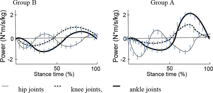
The data in Figure 3 show the difference in the manifestation of the joint power of the lower limb during the stance phase in a running step at a speed of 3 m/s for groups A and B, which can characterize the individual style of the running technique. The calculation of the joint power was carried out according to the described algorithm [13], summing the power produced by each muscle in the model serving the corresponding joint (the sign of the direction is taken into account),

Figure 3.

Patterns of joint power for the ankle, knee, and hip joints during the ground contact phase in running 3 m/s.

Table 3 and Figures 4 and 5 outline the kinematic, dynamic and energy data observed for the two groups for the speeds of 5.1 and 3 m/s.

Subject/speed		Peak moment, N m/kg	Peak power, N m/s/kg	Stiffness	Energy transfer from hip to knee, %	Energy transfer from knee to ankle, %	Summary metabolic power consumed, W/kg
Group A	5 m/s	1.72	0.304	13.1	0.52	1.19	9.76
	3 m/s	0.63	0.790	14.1	1.28	1.58	8.76
Group B	5 m/s	1.52	0.44	12.5	2.41	0.58	9.75
	3 m/s	1.32	0.28	9.8	5.5	0.5	4.77

Table 3.

Initial experimental data.

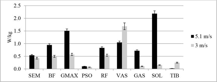
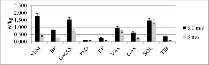
Figure 4.

Comparison of metabolic power consumed (W/kg) for running at 3 and 5.1 m/s (group A) (by Umberger et al. [29, 30] with some modifications [10]).

Figure 5.

Comparison of metabolic power consumed (W/kg) for running at 3 and 5.1 m/s (group B) (by Umberger et al. [29] and Verkhoshansky and Verkhoshansky [30] with some modifications [10]).

Figures 4 and 5 show data characterizing the metabolic power of the main muscles involved in the running step for different running speeds. Расчет metabolic power consumed for muscles in the model was carried out by Umberger et al. [29] and Verkhoshansky and Verkhoshansky [30] with some modifications [10].

3.2 Modeling the change in running technique by modifying the stiffness

From the practical point of view, for the purposes of improvement the running technique and control, one of the key parameters K_leg is the amplitude of knee flexion during the stance phase of a running step. This was achieved by increasing or decreasing the l₀.

To conduct the modeling in this case, we made an assumption of stiffness changing to have an effect on RE. For that purpose, the studied models were changed by increasing or decreasing the leg stiffness by 5% driven by changing the knee angles.

The results in Table 4 demonstrate that increasing stiffness by decreasing the knee angle amplitude for the subjects from group A leads to elevated impact of elastic energy when transferring energy from hip to knee (15%) and from knee to ankle (6.6%). Similar result is observed when decreasing the stiffness—the corresponding changes are 10.4% and 3.3%, respectively.

		Maximum moment, N m/kg	Maximum power, N m/s/kg	Stiffness	Energy transfer from hip to knee, %	Energy transfer from knee to ankle, %	Summary metabolic power consumed, W/kg
Group A	Stiffness increased	1.39	2.0	13.8	0.61	1.23	9.74
	Stiffness decreased	1.59	1.50	12.45	0.58	1.26	9.79
Group B	Stiffness increased	2.15	0.49	13.2	3.18	0.59	9.09
	Stiffness decreased	2.36	0.38	11.85	2.50	0.60	9.82

Table 4.

Modeling data obtained by increasing or decreasing leg stiffness.

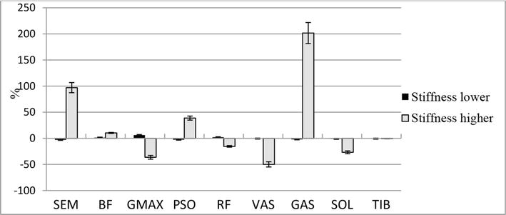
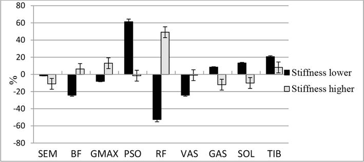
Figures 6 and 7 show changes in the metabolic power of the muscles in the running step with increasing and decreasing stiffness of the leg according to the results of computer simulation.

Figure 6.

The difference (in %) between the values of consumed metabolic power of muscles during the simulation of the stiffness of the supporting leg in group A athletes. Stiffness lower—reduction in leg stiffness by 5%, Stiffness higher—increase in leg stiffness by 5%.

Figure 7.

The difference (in %) between the values of consumed metabolic power of muscles during the simulation of the stiffness of the supporting leg in group B athletes. Stiffness lower—reduction in leg stiffness by 5%, Stiffness higher—increase in leg stiffness by 5%.

3.3 Changing the muscle activity while running toward reducing metabolic costs

In accordance with conducted analysis of experimental data, the second part of the study was targeted for individual editing of muscle excitation patterns for muscles in the lower limbs. This is achieved by using a specific OpenSim tool—Excitation Editor. This is a mandatory step when modeling using the Forward Dynamics approach [15, 33].

For the model experiment, one athlete from each group was selected: the subject SA from group A, the subject PD from group B.

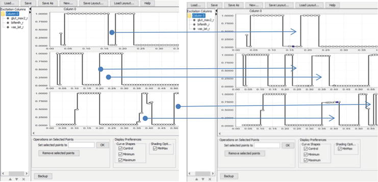
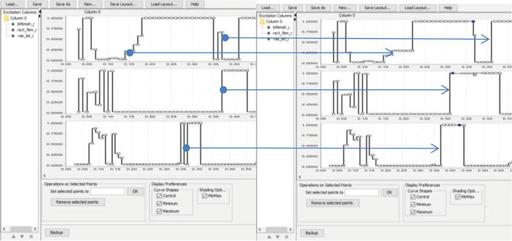
For the PD subject (Figure 8), the muscle activation change was aimed toward a sequential involvement of joints while push-off: first, the hip flexion started, and only later—the knee flexion.

Figure 8.

Example of excitation editor for PD subject from group B. Muscles top to bottom—BF (biceps femoris long head), RF (rectus femoris), VAS (vastus medialis); on the left—simulating muscle activity before making changes; on the right—simulation of muscle activity after making changes. Arrows show changes in muscle activity.

Making changes to the muscle activity patterns (Figures 8 and 9) leads to changes in the results of output indicators (Table 5). An increase in muscle coactivation in an SA athlete leads to an increase in the stiffness of the supporting leg by 1.5%. At the same time, an increase in leg stiffness reduces the value of torque and maximum power by 5.3 and 3.3%, respectively. Also, the SA athlete has reduced energy transfer between joints by 7.7% from hip to knee and by 5.3% from knee to ankle. A different situation is observed in the PD athlete, in whom conditions were created in the model to increase the time of work of the biarticular muscles. As a result of such changes, in the PD athlete, the stiffness of the muscles of the supporting leg, in contrast to the SA athlete, decreases by 2.4%. Accordingly, there is an increase in both torque and maximum power by 6.2% and 4.4%, respectively. Noteworthy is the increase in ESE between the joints by 67.2% from hip to knee and by 81.9% from knee to ankle. Such a relationship in running between leg stiffness, moment of force and power is noted by other authors [24]. Despite the opposite changes in the output data of both athletes, the total metabolic costs are reduced in the SA athlete by 9.3% and by 5.5% in the PD athlete.

Figure 9.

Example of excitation editor for SA subject from group A. Muscles top to bottom—BF, RF, VAS; on the left—simulating muscle activity before making changes; on the right—simulation of muscle activity after making changes. Arrows show changes in muscle activity.

		Maximum moment, N m/kg	Maximum power, N m/s/kg	Stiffness	Energy transfer from hip to knee, %	Energy transfer from knee to ankle, %	Summary metabolic power consumed, W/kg
SA	Before (original)	1.72	0.304	13.1	0.52	1.19	9.76
	Modeled (changed)	1.63	0.291	13.3	0.48	1.23	8.86
PD	Before (original)	1.52	0.44	12.5	2.41	0.58	9.75
	Modeled (changed)	1.62	0.46	12.2	7.34	4.78	8.24

Table 5.

Modeling data obtained when increasing or decreasing the leg stiffness for subject.

4. Discussion

Experimental laboratory testing of athletes revealed the features of the running step technique, dividing them into groups A and B (Figure 3). The difference in running technique is based on the results of earlier studies [13, 14, 25, 34]. Athletes in group A in running use the “catapult” mechanism, in which the transfer of energy between the joints is carried out with the help of biarticular muscles. When performing repulsion while running, athletes of group B use the effect of accumulation and release of elastic deformation energy.

The data in Table 3 show that group A during the 5.1 m/s run had low peak power (the sum of hip, knee and ankle joint powers of the leg that contacts with the surface) while having a high peak moment in the same group of joints. For the 3 m/s run the same subject demonstrates high aggregated joint moment, while the aggregated power is significantly decreasing. Both speeds have similar muscle metabolic costs and stiffness.

These data suggest a significant change of running style for the two speeds. Subject from group A has strong isometric force capabilities for the knee muscles (Table 1). For the lower speed the subject uses his force abilities and demonstrates high stiffness of the leg touching the surface. The stiffness is driven by the large amounts of work performed by the muscles on the back side of the leg—SEM, BF, GMAX and SOL (Figure 3). The subject, however, does not use elastic strain energy. The muscle usage drives high metabolic costs and is linked to the usage of “catapult” mechanism. The “catapult” is explained by the energy transfer via bi-articular muscles. Strong monoarticular gluteus muscles, in particular, m. gluteus maximus (GMAX), play a major role in hop extension. Power from GMAX is transferred to a knee joint via a bi-articular m. rectus femoris (RF); knee joint extension is performed by RF and a group of monoarticular m. vastus (VAS). Extension in a knee joint causes plantar flexion in an ankle joint due to energy transfer via m. gastrocnemius (GAS), thus contributing to contraction of a triceps muscle of calf. This mechanism was described in few studies devoted to examination of biomechanics of running, hopping and vertical jumps [13, 14, 25, 35, 36].

In contrast to the 3 m/s run, while running at 5.1 m/s the subject does not use the “catapult” mechanism, and the excentric mode work is largely performed by the thigh de-flexion muscles (VAS). The GAS and SOL muscles are almost not used in the movement due to their low metabolic outputs (Figure 2), i.e. the “force” push-off option is used.

Compared to group A, for group B we have observed lower peak joint moments and peak powers, as well as lower stiffness while running. However, the usage % of ESE is much higher (Table 2), especially for running at the speed of 3 m/s. This leads to lower metabolic costs at the speed of 3 m/s. At the same time, for the 5.1 m/s experiment, the 2-time decrease of ESE usage leads to almost 2-time increase in the metabolic costs. Group B, compared to group A, does not change the technique from one speed to another, which is proven by the same muscle usage (Figure 3). ESE usage decrease for 5 m/s can be explained by elevated work of the hamstrings (SEM, BF and GMAX), which is connected to lower power capacity of the subject (Table 3). Push-off is performed by lowering the muscle contraction rate, but this leads to increase of the leg stiffness, which, in result, leads to increased metabolic costs.

It is worth mentioning that ESE transfer from joint to joint is achieved using a different mechanism: the mechanism of energy transfer by bi-articular muscles. The mechanism of energy transfer starts working when a bi-articular muscle is operating in concentric regime. However, when it operates in an almost isometric regime (i.e. very low speed of contraction), it can develop a greater force [25]. Furthermore, bi-articular muscles help involve monoarticular muscles into performing in the optimal way in order to achieve the most effective energy usage [37].

This metric can be used to estimate the stiffness of the leg. Intuition tells us that vertical fluctuations have negative effect on energy economy. Dalleau et al. [34], Arampatzis et al. [18] emphasized the importance of neuro-muscular factors and demonstrated that RE depends on the leg stiffness, with higher stiffness leading to better RE. Similarly, Williams and Cavana [38] have shown the tendency (albeit, small) toward smaller vertical fluctuations and better RE.

However, we do not observe a decrease in total muscle metabolic costs, since in absolute values the changes are too small. For running exercise, the change of the stiffness is connected with the increase of required power through increasing the work of two-joint GAS muscle (Figure 5). Presumably, the same fact for lower stiffness can be explained by larger preemptive flexion of muscles in the amortization phase.

For subjects from group B, when we increase stiffness the sum join moment is also increased because of significant bump (24.2%) in ESE component. This model behavior leads to a significant decrease in the overall metabolic cost (7.7%). If we lower the stiffness the metabolic cost is highly increased, because in this case we have to stress the muscles that de-flex knee and hip joints (RF) and additional use the hip flexion muscles (PSO)—see Figure 6.

The stiffness change modeling demonstrated that the metabolic cost impact of these changes is heavily dependent on subject’s individual characteristics. For the subjects from group A, who is better strength capacity and uses the “catapult” energy transfer approach, it is very difficult to change and adapt the running technique. This leads to extra metabolic costs. The subjects from group B, changing the technique leads to a better energy economy.

A forward dynamics (FD) simulation is the integration of the differential equations that define the dynamic behavior of a musculoskeletal model with revised (modified) muscle activation data for predetermined time intervals. In contrast to inverse dynamics, where the motion of the model was known and the forces and torques responsible for the motion were required, FD is a mathematical model that outlines how coordinates and their velocities change due to the application of forces and torques (moments). The modeling for this part of the experiment was performed only for the running speeds of 5.1 m/s aimed to lower the total metabolic cost.

For the two studied cases, the following assumptions were used. For the SA subject (Figure 7), the introduced muscle changes were aimed to increase the leg stiffness by co-activation of “antagonist” muscles when transferring from the concentric muscle regime to eccentric muscle regime.

Calculations for individual muscles demonstrated that the most drastic drop in metabolic cost for SA subject is concentrated in the muscles responsible for body stabilization—PSO, SEM. For PD subject, the calculations outlined that the highest metabolic cost reduction is linked to RF and VAS muscles. This can be explained by the fact that the modeling muscle activation was aimed to decrease the impact of antagonist muscles.

The technology is based on using a regulated testing procedure aimed to discover individual characteristics of an athlete, not only of his/her technique, but also of the related physiological functional systems abilities. Then we use computer modeling with pre-selected criteria for motion optimization in order to achieve the best result. This data allows us to select the options, training method aimed to correct specific areas. During this time the target (end) result is known, which makes it a more structured approach.

Limitations that exist in this study should be noted. Firstly, in a computer simulation experiment, one successful option for calculating the direct dynamics, found by manual selection, is presented. Secondly, we must take into account that the above statements can only be extrapolated to performing cyclic running exercises on a flat surface. At the same time, the biathlon tracks pass through rough terrain. The model presents only a limited number of skeletal muscles and their characteristics of contractile behavior. Potential differences in the functioning of the fast and slow muscle fibers of the contracting muscle are not taken into account. However, the present model can also form the basis of a more complex model, which includes the behavior of other physiological systems (cardiovascular, respiratory). Thus, it can be used to study the contribution to which the variability in the behavior of these systems introduces certain limitations in the use of biomechanical mechanisms to save metabolic costs in running. Future studies can use the developed methodology in this study to determine the individual characteristics of the locomotion technique and use this information to develop special strength and coordination programs to improve athletic performance and reduce the risk of injuries.

5. Conclusion

Despite the limitations of our work, we believe that two important conclusions can be drawn from this study. First, it is defined that top-class athletes in cyclic endurance disciplines tend to use various biomechanical mechanisms for performing movements. Despite the fundamental difference in the organization of these mechanisms, they can equally be used to reduce metabolic costs.

Our second finding is that our model of muscle energy expenditure provides greater insight than simpler measures based solely on raw instrumental data on muscle activation (electromyography data) or measurements of mechanical joint power and/or the Center of Mass from tensometry data. Computer models of muscle energy allow us to study energy consumption with unprecedented accuracy, complementing the indirect calorimetric measurements obtained experimentally at the whole body level.

This research shows that modern hardware and the modern computer technologies can be used to enable ‘pin-point’ engineering approach for training purposes, including constructing highly accurate forecasts for each athlete depending on the suggested training activities—ultimately leading to greater results in professional sport.

References

1.Hamner SR, Delp SL. Muscle contributions to fore-aft and vertical body mass center accelerations over a range of running speeds. Journal of Biomechanics. 2013;46(4):780-787
2.Gleim GW, Stachenfeld NS, Nicholas JA. The influence of flexibility on the economy of walking and jogging. Journal of Orthopaedic Research. 1990;8:814-823
3.Kyrolainen H, Belli A, Komi PV. Biomechanical factors affecting running economy. Medicine & Science in Sports & Exercise. 2001;33:1330-1337
4.Laaksonen MS, Andersson E, Jonsson Kårström M, Lindblom H, McGawley K. Laboratory-based factors predicting skiing performance in female and male biathletes. Frontiers in Sports and Active Living. 2020;2:99. DOI: 10.3389/fspor.2020.00099
5.Luchsinger H, Talsnes RK, Kocbach J, Sandbakk Ø. Analysis of a biathlon Sprint competition and associated laboratory determinants of performance. Frontiers in Sports and Active Living. 2019;1:60. DOI: 10.3389/fspor.2019.00060
6.Wilson AM, Watson JC, Lichtwark GA. Biomechanics: A catapult action for rapid limb protraction. Nature. 2003;421(6918):35-36. DOI: 10.1038/421035a
7.Kram R, Taylor CR. Energetics of running: A new perspective. Nature. 1990;346:265-267
8.Kuo AD. The six determinants of gait and the inverted pendulum analogy: A dynamic walking perspective. Human Movement Science. 2007;26:617-656
9.Margaria R, Cerretelli P, Aghemo P, Sassi G. Energy cost of running. Journal of Applied Physiology. 1963;18:367-370
10.Uchida TK, Hicks JL, Dembia CL, Delp SL. Stretching your energetic budget: How tendon compliance affects the metabolic cost of running. PLoS One. 2016;11:e0150378. DOI: 10.1371/journal.pone.0150378
11.Cavagna GA, Heglund NC, Taylor CR. Mechanical work in terrestrial locomotion; two basic mechanisms for minimizing energy expenditure. The American Journal of Physiology. 1977;233:R243-R261
12.Pandy MG, Zajac FE. Optimal muscular coordination strategies for jumping. Journal of Biomechanics. 1991;24:1-10
13.Prilutsky BI, Zatsiorsky VM. Tendon action of two-joint muscles: Transfer of mechanical energy between joints during jumping, landing, and running. Journal of Biomechanics. 1994;27(1):25-34
14.Prilutsky BI, Petrova LN, Raitsin LM. Comparison of mechanical energy expenditure of joint moments and muscle forces during human locomotion. Journal of Biomechanics. 1996;29(4):405-415
15.Delp SL, Anderson FC, Arnold AS, Loan P, Habib A, John CT, et al. OPENSIM: Open-source software to create and analyze dynamic simulations of movement. IEEE Transactions on Biomedical Engineering. 2007;54(11):1940-1950
16.Beaver W, Wasserman K, Whipp B. A new method for detecting anaerobic threshold by gas exchange. Journal of Applied Physiology. 1986;60(6):2020-2027
17.Seger JY, Westing SH, Hanson M, Karlson E, Ekblom B. A new dynamometer measuring concentric and eccentric muscle strength in accelerated, decelerated, or isokinetic movements. Validity and reproducibility. European Journal of Applied Physiology and Occupational Physiology. 1988;57(5):526-530. DOI: 10.1007/BF00418457
18.Arampatzis A, Knicker A, Netzler V, Brügemann G-P. Mechanical power in running: A comparison of different approaches. Journal of Biomechanics. 2000;33:457-463
19.Cavagna GA. Storage and utilization of elastic energy in skeletal muscle. Exercise and Sport Sciences Reviews. 1977;5:89-129
20.Heglund NC, Fedak MA, Taylor CR, Cavagna GA. Energetics and mechanics of terrestrial locomotion IV. Total mechanical energy changes as a function of speed and body size in birds and mammals. The Journal of Experimental Biology. 1982;97:57-66
21.Hoffer JA, Andreassen S. Regulation of soleus muscle stiffness in premammillary cats: Intrinsic and reflex components. Journal of Neurophysiology. 1981;45(2):267-285. DOI: 10.1152/jn.1981.45.2.267
22.Günther M, Blickhan R. Joint stiffness of the ankle and the knee in running. Journal of Biomechanics. 2002;35(11):1459-1474. DOI: 10.1016/s0021-9290(02)00183
23.Mauroy G, Schepens B, Willems PA. Leg stiffness and joint stiffness while running to and jumping over an obstacle. Journal of Biomechanics. 2014;47(2):526-535. DOI: 10.1016/j.jbiomech.2013.10.039
24.Nummela A, Keranen T, Mikkelsson LO. Factors related to top running speed and economy. International Journal of Sports Medicine. 2007;28:655-661
25.Bobbert MF, van Soest JJ. Two-joint muscles offer the solution, but what was the problem? Motor Control. 2000;4:48-52
26.Hamner SR, Seth A, Delp SL. Muscle contributions to propulsion and support during running. Journal of Biomechanics. 2010;43(14):2709-2716
27.Handsfield GG, Meyer CH, Hart JM, Abel MF, Blemker SS. Relationships of 35 lower limb muscles to height and body mass quantified using MRI. Journal of Biomechanics. 2014;47:631-638
28.Thelen DG, Anderson FC, Delp SL. Generating dynamic simulations of movement using computed muscle control. Journal of Biomechanics. 2003;36:321-328
29.Umberger BR, Gerritsen KGM, Martin PE. A model of human muscle energy expenditure. Computer Methods in Biomechanics and Biomedical Engineering. 2003;6:99-111. DOI: 10.1080/1025584031000091678
30.Verkhoshansky YV, Verkhoshansky N. Special Strength Training: Manual for Coaches. Rome: Verkhoshansky SSTM; 2011
31.Uchida TK, Seth Uchida TK, Seth A, Pouya S, Dembia CL, Hicks JL, et al. Simulating ideal assistive devices to reduce the metabolic cost of running. PLoS One. 2016;11(9):e0163417. DOI: 10.1371/journal.pone.0163417
32.Bullimore SR, Burn JF. Consequences of forward translation of the point of force application for the mechanics of running. Journal of Theoretical Biology. 2006;238:211-219
33.Delp SL, Loan JP, Hoy MG, Zajac FE, Topp EL, Rosen JM. An interactive graphics-based model of the lower extremity to study orthopedic surgical procedures. IEEE Transactions on Biomedical Engineering. 1990;37:757-767
34.Dalleau G, Belli A, Bourdin M, Lacour J-R. The spring-mass model and the energy cost of treadmill running. European Journal of Applied Physiology. 1998;77:257-263
35.de Graaf JB, Bobbert MF, Tetteroo WE, Ingen SG, I. van. Mechanical output about the ankle in countermovement jumps and jumps with extended knee. HMS. 1987;6:333-347
36.Iida F, Rummel J, Seyfarth A. Bipedal walking and running with spring-like biarticular muscles. Journal of Biomechanics. 2007;41(3):656-667. DOI: 10.1016/j.jbiomech.2007.09.033
37.van Leeuwen JL, Spoor CW. On the role of biarticular muscles in human jumping. Journal of Biomechanics. 1992;25(2):207-209
38.Williams KR, Cavanagh PR. Relationship between distance running mechanics, running economy and performance. Journal of Applied Physiology. 1987;63:1236-1245
Written By
Mikhail Shestakov and Alexander Korchagin
Submitted: 24 May 2023Reviewed: 17 June 2023Published: 13 November 2023