Kantowski-Sachs Barrow Holographic Dark Energy Model in Saez-Ballester Theory of Gravitation

Abstract

In this chapter, we have studied a spatially homogeneous and anisotropic Kantowski-Sachs universe in the presence of Barrow Holographic Dark Energy in the background of Saez-Ballester scalar-tensor theory of gravitation. To find the exact solution of the SB field equations, we have assumed that the shear scalar is directly proportional to the expansion scalar. This assumption leads to relation between metric potentials of the models. We have discussed non-interacting and interacting cosmological models. Moreover, we have discussed several cosmological parameters such as energy densities of DM and DE (${\rho }_m$ & ${\rho }_b$), deceleration $\left(q\right)$, equation of state (${\omega }_b$) and skewness ($\alpha$) parameters, squared sound speed ($v_s^2$), ${\omega }_b$-${\omega }_{b^{\prime }}$ plane statefinders and $\mathit{Om}$-diagnostics parameters through graphical representation for both the interacting models. Also, we have observed that the current values of deceleration and EoS parameters of our constructed models coincide with the recent observational data.

1. Introduction

The modern cosmological evidence [1, 2, 3, 4] indicated that there is an accelerated expansion. The responsible cause behind this accelerated expansion is a miscellaneous element having exotic negative pressure termed as Dark Energy (DE). The nature and the cosmological origin of DE are still enigmatic. To describe the phenomenon of DE, several models have been presented. According to several findings, DE should behave like a fluid with ‘negative pressure, counterbalancing the action of gravity, and speeding up the universe’ [5, 6]. The general methodology is to define the dynamics of the universe by assuming the source of DE is represented as a non-zero “cosmological constant $\mathrm{\Lambda }$,” connected to “vacuum quantum field fluctuations” [7, 8]. One proposed solution to DE is the cosmological constant $\mathrm{\Lambda }$. However, there are difficulties related to its theoretically predicted order of magnitude relative to that of the observed vacuum energy [9]. Other solutions [10, 11, 12, 13, 14, 15] go to the idea that cosmic acceleration may be caused by a modification in gravity, perhaps General Relativity (GR) is not valid on cosmological scales.

Hooft [16] has proposed a new dark energy model, known as the Holographic Dark Energy (HDE) model, which was based on the Holographic Principle (HP) and some features of quantum gravity theory. The holographic principle states that the number of degrees of freedom of a gravity-dominated system must vary along with the area of the surface bounding the system [17, 18]. For a system with size $L$, it is required that the total energy in a region of size $L$ should not exceed the mass of a black hole of the same size for the quantum zero-point energy density associated with the UV cutoff, thus $L^2{\rho }_b\le M_p^2$, where ${\rho }_b$ is the vacuum energy density caused by UV cutoff, $M_p$ is the reduced Planck mass given by the relation $M_p\approx \frac{1}{8\mathit{\pi G}}$ and $L$ is the IR cutoff. The HDE model with Hubble horizon as an IR cutoff is not able to explain the current accelerated expansion [19, 20]. However, the HDE models with other IR cutoffs, e.g., particle horizon, event horizon, apparent horizon, etc. describe the accelerated phenomena of the evolution of the Universe and are in agreement with the observational data [21, 22, 23, 24, 25, 26, 27]. Sadri and Khurshudyan [28] have analyzed the HDE model with the Hubble horizon as an IR cutoff in the framework of the flat FRW model while taking into account the non-gravitational interaction between DM and HDE, which is able to explain the current accelerated expansion.

2. Body of the manuscript

Barrow [29, 30] has recently found the possibility that the surface of a black hole could have a complex structure down to arbitrarily tiny due to quantum-gravitational effects. The above potential impacts of the quantum-gravitational space-time form on the horizon region would therefore prompt another black hole entropy relation, the basic concept of black hole thermodynamics. In particular

$$S_B={\left(\frac{A}{A_0}\right)}^{1+\frac{\mathrm{\Delta }}{2}},$$E1

Here $A$ and $A_0$ stand for the normal horizon area and the Planck area, respectively. The new exponent $\mathrm{\Delta }$ is the quantum-gravitational deformation with bound as $0\le \mathrm{\Delta }\le 1$ [29, 30, 31, 32, 33]. The value $\mathrm{\Delta }=1$ gives to the most complex and fractal structure, while $\mathrm{\Delta }=0$ relates to the easiest horizon structure. Here as a special case, the standard Bekenstein-Hawking entropy is re-established and the scenario of Barrow Holographic Dark Energy (BHDE) has been developed. The BHDE models have been explored and discussed by various authors [34, 35, 36, 37, 38] in various other contexts. The energy density of BHDE is expressed as

$${\rho }_b={\mathit{CH}}^{2-\mathrm{\Delta }},$$E2

where $C$ is an unknown parameter and $\mathrm{\Delta }>0$.

Nandhida and Mathew [39] have considered the Barrow Holographic Dark Energy as a dynamical vacuum, with Granda-Oliveros (GO) length as IR cut-off and studied the evolution of cosmological parameters with the best-estimated model parameters extracted using the combined data-set of supernovae type Ia pantheon (SN-Ia) and observational Hubble’s data. Bhardwaj et al. [40] have studied statefinder hierarchy model for the BHDE. Adhikary et al. [41] have constructed a BHDE in the case of non-at universe in particular, considering closed and open spatial geometry and observed that the scenario can describe the thermal history of the universe, with the sequence of matter and DE epochs. Considering BHDE Sarkar and Chattopadhyay [42] reconstruct modified gravity as the form of background evolution and point out that the equation of state can have a transition from quintessence to phantom with the possibility of Little Rip singularity. Saridakis [43] has studied modified cosmology through spacetime thermodynamics and Barrow horizon entropy. Koussour et al. [44, 45] have investigated Bianchi type $I$ BHDE model and the stability analysis in symmetric teleparallel gravity.

Shamir and Bhatti [46] have analyzed anisotropic DE Bianchi type $\mathit{III}$ cosmological models in Brans-Dicke (BD) theory of gravity. Aditya and Reddy [47] have investigated anisotropic new HDE model in the framework of SB theory of gravitation. Jawad et al. [48] have discussed cosmological implications of Tsallis DE in modified BD theory. Santhi and Sobhanbabu [49, 50] have studied anisotropic THDE models in Scalar tensor theories of gravitation. Sobhanbabu and Santhi [51] have investigated anisotropic MHDE models with sign-changeable interaction in a scalar-tensor theory of gravitation. Recently, Sharif and Majid [52] have studied isotropic and complexity-free deformed solutions in self-interacting in a BD theory of gravitation. Very recently, Pradhan et al. [53] have studied FRW cosmological models with BHDE in the background of scalar-tensor theory of gravitation.

3. Metric and SB field equations

We consider a homogeneous and anisotropic KK Universe described by the line-element

$${\mathit{ds}}^2={\mathit{dt}}^2-X^2\left(t\right){\mathit{dr}}^2-Y^2\left(t\right)\left(d{\theta }^2+{sin}^2\mathit{\theta d}{\varphi }^2\right),$$E3

where $X\left(t\right)$ and $Y\left(t\right)$ are functions of cosmic time $t$ only.

We assume that the Universe is filled by a DM without pressure with energy density $\left({\rho }_m\right)$, and BHDE candidate with energy density (${\rho }_b$). Here we take more general Energy Momentum Tensors for DM and BHDE fluid in the following form:

$$T_{\mu }^{\nu }=\mathit{diag}\left[\mathrm{1,0,0,0}\right]{\rho }_m\mathit{\text{and}}{\overline{T}}_{\mu }^{\nu }=\mathit{diag}\left[1,-{\omega }_b,-\left({\omega }_b+\alpha \right),-\left({\omega }_b+\alpha \right)\right]{\rho }_b,$$E4

where ${\omega }_b=\frac{p_b}{{\rho }_b}$ is equation of state (EoS) parameter of BHDE, ${\rho }_m$ is energy density of DM, $p_b$ and ${\rho }_b$ are pressure and energy density of BHDE, respectively, and $\alpha$ is skewness parameter is in devitation from EoS parameter ${\omega }_b$ on $y$ and $z$ axes, respectively. The SB field equations are

$$R_{\mathit{\mu \nu }}-\frac{1}{2}{\mathit{Rg}}_{\mathit{\mu \nu }}-w{\varphi }^n\left({\varphi }_{,\mu }{\varphi }_{,\nu }-\frac{1}{2}{g}_{\mathit{\mu \nu }}{\varphi }_{,\beta }{\varphi }^{,\beta }\right)=-\left(T_{\mathit{\mu \nu }}+{\overline{T}}_{\mathit{\mu \nu }}\right),$$E5

where $T_{\mathit{\mu \nu }}$ and ${\overline{T}}_{\mathit{\mu \nu }}$ are energy-momentum tensors (EMT) for DM and DE, respectively. Scalar field $\varphi$ equation

$$2{\varphi }^n{\varphi }_{,\mu }^{,\mu }+n{\varphi }^{n-1}{\varphi }_{,\beta }{\varphi }^{,\beta }=0,$$E6

and energy conservation equations are

$${\left(T_{\mathit{\mu \nu }}+{\overline{T}}_{\mathit{\mu \nu }}\right)}_{;\nu }=0,$$E7

where $T_{\mathit{\mu \nu }}$ and ${\overline{T}}_{\mathit{\mu \nu }}$ are EMTs for DM and BHDE, respectively.

The SB field Eq. (5), for KK line-element Eq.(3) with the help of Eq.(4), can be written as

$$2\frac{\ddot{Y}}{Y}+\frac{{\dot{Y}}^2}{Y^2}+\frac{1}{Y^2}-\frac{w}{2}{\varphi }^n{\dot{\varphi }}^2=-{\omega }_b{\rho }_b,$$E8

$$\frac{\ddot{X}}{X}+\frac{\ddot{Y}}{Y}+\frac{\dot{X}\dot{Y}}{\mathit{XY}}-\frac{w}{2}{\varphi }^n{\dot{\varphi }}^2=-\left({\omega }_b+\alpha \right){\rho }_b,$$E9

$$2\frac{\dot{X}\dot{Y}}{\mathit{XY}}+\frac{{\dot{Y}}^2}{Y^2}+\frac{1}{Y^2}+\frac{w}{2}{\varphi }^n{\dot{\varphi }}^2=-\left({\rho }_m+{\rho }_b\right),$$E10

$$\ddot{\varphi }+\left(\frac{\dot{X}}{X}+2\frac{\dot{Y}}{Y}\right)\dot{\varphi }+\frac{n}{2}\frac{{\dot{\varphi }}^2}{\varphi }=0.$$E11

We can write the conservation Eq.(7) of the DM and BHDE as

$${\dot{\rho }}_m+\left(\frac{\dot{X}}{X}+2\frac{\dot{Y}}{Y}\right){\rho }_m+{\dot{\rho }}_b+\left(\frac{\dot{X}}{X}+2\frac{\dot{Y}}{Y}\right)\left(1+{\omega }_b\right){\rho }_b+2\alpha \left(\frac{\dot{Y}}{Y}\right){\rho }_b=0,$$E12

where overhead dot (.) denotes ordinary differentiation with respect to cosmic time $t$.

The SB field eqs. (8)–(11) form a system of four (4) non-linear equations with seven (7) unknowns; $X$, $Y$, ${\rho }_m$, ${\rho }_b$, ${\omega }_b$, $\alpha$_, and $\varphi$. In order to solve the field equations explicitly, we need three additional constraints which we will assume in the next section. Now we will know some of the physical and geometric quantities that we will need later.

The average scale parameter of the KK Universe is given by

$$a={\left({\mathit{XY}}^2\right)}^{\frac{1}{3}}.$$E13

The spatial volume of the universe

$$V={\left(a\right)}^3={\mathit{XY}}^2.$$E14

The average Hubble parameter $\left(H\right)$, expansion scalar ($\theta$), and shear scalar (${\sigma }^2$) of KK universe are defined as

$$H=\frac{\dot{a}}{a},\theta =3H,\mathit{\text{and}}{\sigma }^2=\frac{1}{2}\left[{\left(\frac{\dot{X}}{X}\right)}^2+2{\left(\frac{\dot{Y}}{Y}\right)}^2\right]-\frac{{\theta }^2}{6}$$E15

The Deceleration Parameter (DP) $q$ of the KK universe is defined as

$$q=-\frac{a\ddot{a}}{{\dot{a}}^2}$$E16

4. Solution of the field equations and cosmological models

Hence to find the exact solution of the field equations, we have to use some physically viable conditions; The shear scalar (${\sigma }^2)$ is directly proportional to the scalar expansion ($\theta$) which leads to a relationship between metric potentials [54].

$$X=Y^l,$$E17

where $l\ne 1$ is a positive constant and preserves the non-isotropic behavior of the Universe. Also, we assume that the deceleration parameter (DP) $q$ is a function of the Hubble parameter ($H$) [55].

$$q=-1+\mathit{\gamma H},$$E18

where $\gamma$ is an arbitrary constant.

Now using eqs. (16), and (18), we get the exact solution

$$a=e^{\frac{1}{\gamma }\sqrt{2\mathit{\gamma t}+c_1}},$$E19

where $c_2$ is an integration constant and $\gamma$ arbitrary constant. From Eqs. (13), and (19), we found the metric potentials

$$X=e^{\frac{3l}{\gamma \left(l+2\right)}\sqrt{2\mathit{\gamma t}+c_1}},Y=e^{\frac{3}{\gamma \left(l+2\right)}\sqrt{2\mathit{\gamma t}+c_1}}$$E20

From eq. (2), the energy density of BHDE is

$${\rho }_b=C{\left[\frac{1}{\left(2\mathit{\gamma t}+c_1\right)}\right]}^{\frac{2-\mathrm{\Delta }}{2}}$$E21

Thus, the metric corresponding to the metric potentials (20) can be written as

$${\mathit{ds}}^2={\mathit{dt}}^2-e^{\frac{6l}{\gamma \left(l+2\right)}\sqrt{2\mathit{\gamma t}+c_1}}{\mathit{dr}}^2-e^{\frac{6}{\gamma \left(l+2\right)}\sqrt{2\mathit{\delta t}+c_2}}\left(d{\theta }^2+{sin}^2\theta d{\varphi }^2\right)$$E22

From eqs. (10), (11), (20), and (21), we found the skewness parameter ($\alpha$) is

$$\alpha =\frac{1}{C}\left[\frac{9\left(1-l^2\right)H^{-1}+3\gamma \left(l+2\right)\left(l-3\right)}{{\left(l+2\right)}^2{H}^{-\frac{3}{2}}}+\frac{9\left(1-l\right)}{{\left(l+2\right)}^2{H}^{-\frac{1}{2}}}+e^{-\frac{6}{\gamma \left(l+2\right)H}}\right]H^{\mathrm{\Delta }-2}$$E23

The scalar field $\varphi$ is

$$\varphi ={\varphi }_0\left(\frac{n+2}{2}\right)\int e^{\frac{-3}{\gamma }\sqrt{2\mathit{\gamma t}+c_1}}\mathit{dt},$$E24

where ${\varphi }_0$ is an integration constant.

The plot of DP ($q$) against redshift ($z$) is shown in Figure 1. We have observed that the DP ($q$) passes from positive to negative value as the redshift increase and it approaches to $-1$ at $z=-1$. Thus, our model of the Universe goes from an early deceleration region ($q>0$) to a current acceleration region ($q>0$). Also, we have observed that the current values of $q$ is consistent with recent observational data.

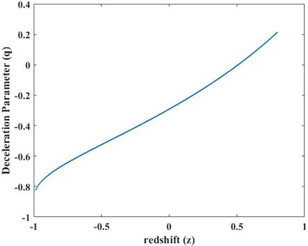
Figure 1.

Variation of deceleration parameter $q$ versus redshift ($z$) for $l=1.995$, $c_2=1$, $w=1000$, and $c_3=1$ of all models.

4.1 Non-interacting BHDE in the SB cosmology

First, we consider that two fluids (DM and BHDE) do not interact with each other. Hence the conversation eq. (14), of the fluids may be conserved separately. The conservation eq. (14) of barotropic fluid leads to

$${\dot{\rho }}_m+3H{\rho }_m=0,$$E25

whereas the conservation eq. (14) BHDE leads to

$${\dot{\rho }}_b+3H\left(1+{\omega }_b\right){\rho }_b+2{\mathit{\alpha \rho }}_b\frac{\dot{Y}}{Y}=0$$E26

From eq. (21) by using eqs. (20), (21), and (23), we get the EoS parameter

$${\omega }_b=-1-\left(\frac{2-\mathrm{\Delta }}{3H^2}\right)\dot{H}-\left(\frac{2}{l+2}\right)\alpha ,$$E27

where $\dot{H}=-\frac{\gamma }{{\left(\sqrt{2\mathit{\gamma t}+c_1}\right)}^{\frac{3}{2}}}$ and $\alpha =\frac{1}{C}\left[\frac{9\left(1-l^2\right)H^{-1}+3\gamma \left(l+2\right)\left(l-3\right)}{{\left(l+2\right)}^2{H}^{-\frac{3}{2}}}+\frac{9\left(1-l\right)}{{\left(l+2\right)}^2{H}^{-\frac{1}{2}}}+e^{-\frac{6}{\gamma \left(l+2\right)H}}\right]H^{\mathrm{\Delta }-2}$.

The evolution of DM and BHDE densities with redshift ($z$) is depicted in Figures 2 and 3 for various values of $\mathrm{\Delta }$, we can see that DM and BHDE densities are positive and increasing functions of redshift $z$ throughout the evolution of the Universe at the present epoch.

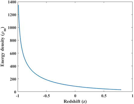
Figure 2.

Variation of energy density (${\rho }_m$) of DM versus redshift ($z$) for $l=1.995$, $c_2=1$, $w=1000$, and $c_3=1$ of all models.

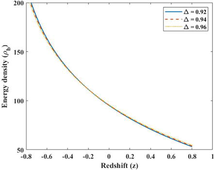
Figure 3.

Variation of energy density (${\rho }_b$) of BHDE versus redshift ($z$) for.

In Figure 4, we have plotted the behavior of skewness parameter ($\alpha$) versus redshift ($z$). It can be seen that the skewness parameter decreasing with an increase in redshift ($z$) but throughout evolution the skewness parameter ($\alpha$) is positive.

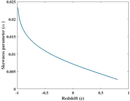
Figure 4.

Variation of skewness parameter ($\alpha$) versus redshift ($z$) for.

In Figure 5, we observed the dynamics of the EoS parameter (${\omega }_b$) against redshift ($z$) for three various values of $\mathrm{\Delta }=0.920.940.96$. The EoS parameter classifies the expansion of the Universe. The EoS parameter ${\omega }_b$ of the BHDE for the non-interacting model completely varies in quintessence region ($-1<{\omega }_b<-\frac{1}{3}$). The current values of ${\omega }_b$ are consistent with Planck observational data.

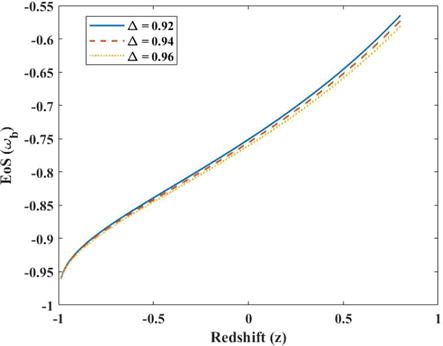
Figure 5.

Variation of equation of state parameter ${\omega }_b$ versus redshift ($z$) for.

4.2 ${\omega }_b-{{\omega }_b}^{\text{'}}$ plane

Caldwell and Linder [56] have pointed out that the quintessence phase of DE can be separated into two distinct regions, that is, thawing (${\omega }_{b^{\prime }}>0$, ${\omega }_b<0$) and freezing $({\omega }_{b^{\prime }}<0$, ${\omega }_b<0)$ regions through ${\omega }_b$-${\omega }_{b^{\prime }}$ plane. Applying the derivative of Eq. (22) with respect to $lna$, we have

$${{\omega }_b}^{\text{'}}=\frac{\left(\mathrm{\Delta }-2\right)\left(H\ddot{H}-2{\dot{H}}^2\right)}{3H^4}-\frac{2\dot{\alpha }}{\left(l+2\right)H},$$E28

where $\dot{\alpha }=\frac{1}{C}\left[\frac{1}{{\left(l+2\right)}^2}\left(9\left(l^2-1\right)H^{-\frac{1}{2}}+\frac{3}{2}\left(9\left(1-l^2\right)H^{-1}+3\gamma \left(l+2\right)\left(l-3\right)\right)H^{\frac{1}{2}}\right)+\frac{9\left(1-l\right)}{{\left(l+2\right)}^2}{H}^{-\frac{1}{2}}+\right.$ $\left.\frac{6H}{\gamma \left(l+2\right)}{e}^{\frac{-6}{\gamma \left(l+2\right)H^2}}+\left(\mathrm{\Delta }-2\right)\left(\frac{9\left(1-l^2\right)H^{-1}+3\gamma \left(l+2\right)\left(l-3\right)}{{\left(l+2\right)}^2{H}^{-\frac{3}{2}}}+e^{-\frac{6}{\gamma \left(l+2\right)H}}\right)\right]H^{\mathrm{\Delta }-3}\dot{H}$, and $\ddot{H}=\frac{3{\gamma }^2}{{\left(2\mathit{\gamma t}+c_1\right)}^{\frac{5}{2}}}$.

Figure 6 shows the ${\omega }_b-{\omega }_{b^{\prime }}$ plane for the three various values of $\mathrm{\Delta }$. We have observed that our non-interacting BHDE model lies in the freezing region (${\omega }_b<0$ and ${\omega }_{b^{\prime }}<0$). It is noticed that the Universe‘s cosmic expansion accelerates more fastly in this freezing area.

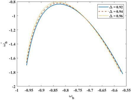
Figure 6.

Variation of ${\omega }_b$ versus ${\omega }_{b^{\prime }}$ of the non-interacting model.

4.3 Stability analysis

We analyze now the stability of the obtained BHDE (non-interacting and interacting) models.

$$v_s^2={\omega }_b+\frac{{\rho }_b}{{\dot{\rho }}_b}{\dot{\omega }}_b$$E29

For our non-interacting BHDE model, squared speed sound $v_s^2$ is given by

$$v_s^2=-1-\left(\frac{2-\mathrm{\Delta }}{3H^2}\right)\dot{H}-\left(\frac{2}{l+2}\right)\alpha +\left(\frac{H\dot{H}}{2-\mathrm{\Delta }}\right){\dot{\omega }}_b$$E30

where ${\dot{\omega }}_b=\frac{\left(\mathrm{\Delta }-2\right)\left(H\ddot{H}-2{\dot{H}}^2\right)}{3H^3}-\frac{2\dot{\alpha }}{l+2},\mathit{\text{here}}\dot{\alpha }=\frac{1}{C}\left[\frac{1}{{\left(l+2\right)}^2}\right.(9\left(l^2-1\right)H^{-\frac{1}{2}}+\frac{3}{2}(9\left(1-1\right)H^{-\frac{1}{2}}+\frac{3}{2}(9\left(1-l^2\right)H^{-1}$

$\left.+3\gamma \left(l+2\right)\left(l-3\right)\left)H^{\frac{1}{2}}\right)+\frac{9\left(1-l\right)}{{\left(l+2\right)}^2}{H}^{-\frac{1}{2}}+\frac{6H}{\gamma \left(l+2\right)}{e}^{\frac{-6}{\gamma \left(l+2\right)H^2}}+\left(\mathrm{\Delta }-2\right)\left(\frac{9\left(1-l^2\right)H^{-1}+3\gamma \left(l+2\right)\left(l-3\right)}{{\left(l+2\right)}^2{H}^{-\frac{3}{2}}}+e^{-\frac{6}{\gamma \left(l+2\right)H}}\right)\right]H^{\mathrm{\Delta }-3}\dot{H}$

For the non-interacting model, Figure 7 shows the evolution of the SSS in terms of redshift ($z$). It is clear that the BHDE non-interacting model is initially unstable $(v_s^2\le 0$) and with cosmic expansion it becomes stable ($v_s^2>0$).

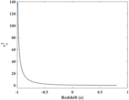
Figure 7.

Variation of squared sound speed $v_s^2$ versus redshift ($z$) of the non-interacting model.

4.4 Interacting BHDE in the SB cosmology

In this case, we focus on the interaction between two dark fluids. Since the nature of both BHDE and DM is still unknown, there is no physical argument to exclude the possible interaction between them. Recently, some observational data shows that there is an interaction between dark sectors [57, 58]. Several authors [59, 60, 61] have investigated the signature of interaction between DE and DM by using optical, $X$-ray, and weak lensing data from the relaxed galaxy clusters. So, it is reasonable to assume the interaction between BHDE and DM in cosmology:

$${\dot{\rho }}_m+3H{\rho }_m=Q,$$E31

whereas the conservation eq. (14) BHDE leads to

$${\dot{\rho }}_b+3H\left(1+{\omega }_b\right){\rho }_b+2{\mathit{\alpha \rho }}_b\frac{\dot{Y}}{Y}=-Q,$$E32

where $Q$ denotes the interaction term between two fluids (DM and BHDE) and we assume the interaction $Q=3\mathit{\beta H}{\rho }_b$, where $\beta$ is coupling parameter:

Now, from eqs. (20), (21), (23), (24), and (32), we found that the EoS parameter is

$${\omega }_b=-1-\beta -\left(\frac{2-\mathrm{\Delta }}{3H^2}\right)\dot{H}-\left(\frac{2}{l+2}\right)\alpha ,$$E33

where $\dot{H}=-\frac{\gamma }{{\left(\sqrt{2\mathit{\gamma t}+c_1}\right)}^{\frac{3}{2}}}$ and $\alpha =\frac{1}{C}\left[\frac{9\left(1-l^2\right)H^{-1}+3\gamma \left(l+2\right)\left(l-3\right)}{{\left(l+2\right)}^2{H}^{-\frac{3}{2}}}+\frac{9\left(1-l\right)}{{\left(l+2\right)}^2{H}^{-\frac{1}{2}}}+e^{-\frac{6}{\gamma \left(l+2\right)H}}\right]H^{\mathrm{\Delta }-2}$

For interacting BHDE model, the EoS parameter (${\omega }_b$) versus redshift $\left(z\right)$ for three various values of $\mathrm{\Delta }$ and $\beta$ are shown in Figures 8–10. We have observed that the EoS parameter starts from the matter-dominated era, then it moves to the quintessence region ($-1<{\omega }_b<-\frac{1}{3}$) and crosses the $\mathrm{\Lambda }\mathit{CDM}$ model (${\omega }_b=-1$), and finally approaches to phantom region (${\omega }_b<-1$). Further, the current values of the EoS parameter (${\omega }_b$) are consistent with recent [62] observational data.

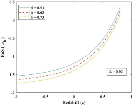
Figure 8.

Variation of ${\omega }_b$ versus redshift ($z$) for interacting model for $\mathrm{\Delta }=0.92$.

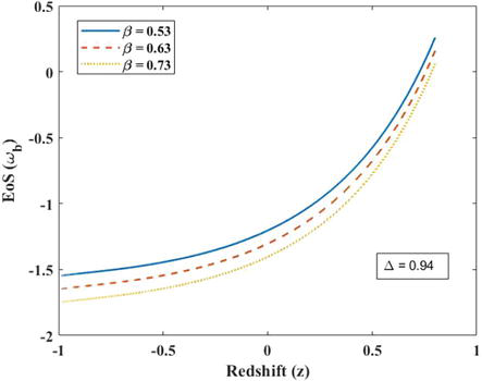
Figure 9.

Variation of ${\omega }_b$ versus redshift ($z$) for interacting model for $\mathrm{\Delta }=0.94$.

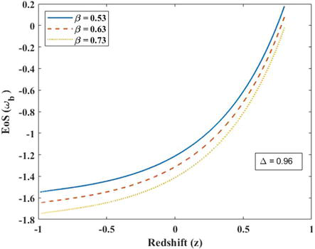
Figure 10.

Variation of ${\omega }_b$ versus redshift ($z$) for interacting model for $\mathrm{\Delta }=0.96.$

Figures 11–13 show the ${\omega }_b-{\omega }_{b^{\prime }}$ plane for the three various values of $\mathrm{\Delta }$ and $\beta$. We have observed that our interacting BHDE model lies in the freezing region (${\omega }_b<0$ and ${\omega }_{b^{\prime }}<0$). It is noticed that the Universe‘s cosmic expansion accelerates more rapidly in this freezing area.

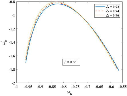
Figure 11.

Variation of ${\omega }_b$ versus ${\omega }_{b^{\prime }}$ of the interacting model.

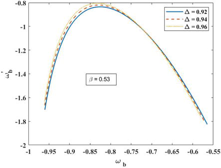
Figure 12.

Variation of ${\omega }_b$ versus ${\omega }_{b^{\prime }}$ of the interacting model.

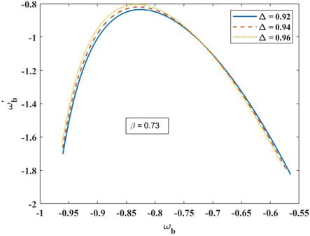
Figure 13.

Variation of ${\omega }_b$ versus ${\omega }_{b^{\prime }}$ of the interacting model.

For our interacting BHDE model, Figure 14 shows the evolution of the SSS in terms of redshift ($z$). It is clear that the interacting BHDE model is initially unstable $(v_s^2\le 0$) and with cosmic expansion it becomes stable ($v_s^2$).

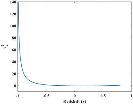
Figure 14.

Variation of squared sound speed ($v_s^2$) versus redshift ($z$) of the interacting models.

4.5 Statefinder diagnostics

In this section, we focus on the diagnosis of the statefinder. The Hubble parameter $H$ represents the Universe’s expansion rate and the deceleration parameter $q$ represents the rate of acceleration or deceleration of the expanding cosmos, which are two well-known geometrical parameters that characterize the Universe‘s expansion history. They only depend on the average scale parameter $a$. This statefinder pairs {r,s} [63, 64] as follows

$$r=\frac{\stackrel{⃛}{a}}{{\mathit{aH}}^3}=\frac{\ddot{H}}{H^3}+3\frac{\dot{H}}{H^2}+1$$E34

$$s=\frac{r-1}{3\left(q-\frac{1}{2}\right)}=\frac{\frac{\ddot{H}}{H^3}+3\frac{\dot{H}}{H^2}}{3\left(q-\frac{1}{2}\right)}$$E35

Figure 15 shows the evolutionary trajectories in $\left\{r,s\right\}$ plane. In the figure, our constructed model lies in the chaplygin gas ($\left\{r>1,s<0\right\}$) model and also meets $\mathrm{\Lambda }$CDM model ($\left\{r=11,s=0\right\}$). Figure 16 depicts that our model lies in Standard Cold Dark Matter (SCDM) region ($\left\{r>1,q>0\right\}$)and also meets $\mathrm{\Lambda }$CDM region ($\left\{r=1,q=0\right\}$).

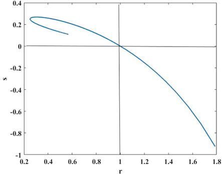
Figure 15.

Variation of statefinder parameters $r$ versus $s$ of the models.

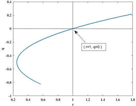
Figure 16.

Variation of statefinder parameters $r$ versus $s$ of the models.

4.6 Om-diagnostic

As a complementary to the statefinder parameters $\left\{r,s\right\}$, a new diagnostic is known as $\mathit{Om}$ studied by some of the researchers [65, 66]. The $\mathit{Om}$ diagnostic parameter for our model is

$$\mathit{Om}\left(x\right)=\frac{h^2\left(x\right)-1}{x^3-1},$$E36

where $x=1+z$ and $h\left(x\right)=\frac{H\left(x\right)}{H_0}$.

The trajectory of Om diagnostics versus redshift (z) is shown in Figure 17. The trajectory reveals that the BHDE model shows initially a positive slope of the trajectory indicating that our model has phantom behavior and the negative slope of the trajectory indicates that our model behavior is quintessence in late time.

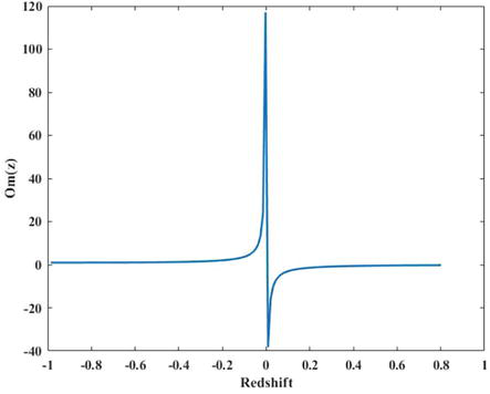
Figure 17.

Variation of statefinder parameters $r$ versus $s$ of the models.

5. Conclusions

In this chapter, we have investigated the accelerated expansion by assuming the BHDE Universe within the framework of SB scalar-tensor theory of gravity. We have investigated various cosmological parameters to analyze the viability of the models and our conclusions are the following:

The deceleration parameter ($q$) passes from positive to negative value as the redshift increase and it approaches to $-1$ at $z=-1$. Thus, our model of the Universe goes from an early deceleration region ($q>0$) to a current acceleration region (Figure 1). The parameter ($q$) of our model consistent with the current observational data are, Capozziello et al. [67], given as

$$q=-0.6401\pm 0.187\left(\mathit{BAO}+\mathit{\text{Masers}}+\mathit{\text{TDSL}}+\mathit{\text{Panthelon}}+H_0\right)$$

$$q=-0.930\pm 0.218\left(\mathit{BAO}+\mathit{\text{Masers}}+\mathit{\text{TDSL}}+\mathit{\text{Panthelon}}+H_z\right).$$

For our non-interacting model, the energy densities of DM and BHDE are positive and increasing function of redshift $z$ throughout the evolution of the Universe at the present epoch (Figures 2 and 3). The skewness parameter decreasing with increase in redshift ($z$) but throughout evolution the skewness parameter ($\alpha$) is positive (Figure 4). The EoS parameter ${\omega }_b$ of the BHDE for non-interacting model completely varies in quintessence region ($-1<{\omega }_b<-\frac{1}{3}$) for three different values of $\mathrm{\Delta }=0.920.940.96$. The current values of ${\omega }_b$ are consistent with Planck [62] observational data (Figure 5). The ${\omega }_b-{\omega }_{b^{\prime }}$ plane for the three various values of $\mathrm{\Delta }$ we observe that our non-interacting BHDE model lies in the freezing region (${\omega }_b<0$ and ${\omega }_{b^{\prime }}<0$). It is noticed that the Universe‘s cosmic expansion accelerates more fastly in this freezing area (Figure 6). The SSS is initially unstable $(v_s^2\le 0$) and with cosmic expansion, it becomes stable ($v_s^2$) for non-interacting BHDE model (Figure 7).

For interacting BHDE model, the EoS parameter starts from the matter dominated era, then it moves to the quintessence region ($-1<{\omega }_b<-\frac{1}{3}$) and crosses the $\mathrm{\Lambda }\mathit{CDM}$ model (${\omega }_b=-1$), and finally approaches to phatom region (${\omega }_b<-1$) for three different values of $\mathrm{\Delta }$ and $\beta$. Also, it is worthwhile to mention here that the present values of the EoS parameter of our BHDE models are in agreement with the modern Plank observational data given by Aghanim et al. [62]. It gives the constraints on the EoS parameter of dark energy as follows:

$$\begin{array}{c}{\omega }_b=-{1.56}_{-0.48}^{+0.60}\left(\mathit{\text{Planck}}+\mathit{TT}+\mathit{\text{lowE}}\right)\\ {\omega }_b=-{1.58}_{-0.41}^{+0.52}\left(\mathit{\text{Planck}}+\mathit{TT},\mathit{EE}+\mathit{\text{lowE}}\right)\\ {\omega }_b=-{1.57}_{-0.40}^{+0.50}\left(\mathit{\text{Planck}}+\mathit{TT},\mathit{TE},\mathit{EE}+\mathit{\text{lowE}}+\mathit{\text{lensing}}\right)\\ {\omega }_b=-{1.04}_{-0.10}^{+0.10}\left(\mathit{\text{Planck}}+\mathit{TT},\mathit{TE},\mathit{EE}+\mathit{\text{lowE}}+\mathit{\text{lensing}}+\mathit{BAO}\right)\end{array}$$

It can be observed from Figures 5, 8–10 that the EoS parameter of our models in both non-interacting and interacting cases lie within the above observational limits which shows the consistency of our results with the above cosmological data. We have observed that our interacting BHDE model lies in the freezing region (${\omega }_b<0$ and ${\omega }_{b^{\prime }}<0$) for the three various values of $\mathrm{\Delta }$ and $\beta$. It is noticed that the Universe‘s cosmic expansion accelerates more rapidly in this freezing area (Figures 11–13). The SSS is initially unstable $(v_s^2\le 0$) and with cosmic expansion it becomes stable ($v_s^2$). It is exactly similar to the non-interacting case (Figure 14).

The behavior of $\left\{r,s\right\}$ and $\left\{r,q\right\}$ planes for our model lies in the chaplygin gas ($\left\{r>1,s<0\right\}$) model and meets $\mathrm{\Lambda }$CDM model ($\left\{r=11,s=0\right\}$). The $\left\{r,q\right\}$ plane lies in SCDM region ($\left\{r>1,q>0\right\}$)and also meets $\mathrm{\Lambda }$CDM region ($\left\{r=1,q=0\right\}$). The trajectory of Om-diagnostics reveals that the BHDE model shows initially our model has phantom behavior and quintessence behavior in late time (Figures 15–17).

Finally, we can state that some of the preceding conclusions in KK BHDE model are good agreement with recent observations.

Conflict of interest

The authors declare that they have no known competing financial interests or personal relationships that could have appeared to influence the work reported in this chapter.

Data availability statement

This chapter has no associated data or the data will not be deposited.

References

- 1.
Riess AG et al. Observational Evidence from Supernovae for an Accelerating Universe and a Cosmological Constant. Astronomy Journal. 1998; 116 :1009 - 2.
Perlmutter S et al. Measurements of Ω and Λ from 42 High-Redshift Supernovae. The Astrophysical Journal. 1999; 517 :565 - 3.
Spergel DN et al. First-Year Wilkinson Microwave Anisotropy Probe (WMAP)* Observations: Determination of Cosmological Parameters. Astrophysical Journal of Supplement. 2003; 148 :175 - 4.
Tegmark M et al. Cosmological parameters from SDSS and WMAP. Physics Review D. 2004; 69 :103501 - 5.
Copeland EJ et al. Dynamics of dark energy. International Journal of Modern Physics D: Gravitation; Astrophysics and Cosmology. 2006; 15 :1753 - 6.
Ade PAR et al. Cosmological parameters. Astronomy and Astrophysics. 2016; 594 :A13 - 7.
Perlmutter S et al. Discovery of a supernova explosion at half the age of the Universe. Nature. 1998; 391 :51 - 8.
Schmidt BP et al. The high-z supernova search: measuring cosmic deceleration and global curvature of the universe using type Ia supernovae. The Astrophysical Journal. 1998; 507 :46 - 9.
Riess AG et al. Type ia supernova discoveries at z > 1 from the hubble space telescope: Evidence for past deceleration and constraints on dark energy evolution. The Astrophysical Journal. 2004; 607 :665 - 10.
Barreiro T et al. Quintessence arising from exponential potentials. Physics Review D. 2000; 61 :127301 - 11.
Caldwell et al. Phantom Energy: Dark Energy with ω < −1: Causes a Cosmic Doomsday. Physical Review Letters. 2003;91 :071301 - 12.
Bagla JS et al. Cosmology with tachyon field as dark energy. Physics Review D. 2003; 67 :063504 - 13.
Armendariz-Picon et al. Essentials of k-essence. Physics Review D. 2001; 63 :103510 - 14.
Cognola G et al. Dark energy in modified Gauss-Bonnet gravity: Late-time acceleration and the hierarchy problem. Physics Review D. 2006; 73 :084007 - 15.
Ferraro et al. Modified teleparallel gravity: Inflation without an inflaton. Physics Review D. 2007; 75 :084031 - 16.
‘t Hooft G. Dimensional Reduction in Quantum Gravity. 1993, arXiv e-prints, pp gr-qc/9310026 - 17.
Susskind L. The World as a Hologram. Journal of Mathematical Physics. 1995; 36 :6377 - 18.
Cohen A et al. Effective Field Theory, Black Holes, and the Cosmological Constant. Physical Review Letters. 1999; 82 :4971 - 19.
Hsu SD. Holographic Bound in Quantum Field Energy Density and Cosmological Constant. Physics Letters B. 2004; 594 :13 - 20.
Li M. The Interacting Generalized Ricci Dark Energy Model in Non-Flat Universe. Physics Letters B. 2004; 603 :1 - 21.
Zhang X, Wu FQ. Constraints on holographic dark energy from type Ia supernova observations. Physics Review D. 2005; 72 :043524 - 22.
Feng C et al. Journal of Cosmology and Astroparticle Physics. 2007; 09 :005 - 23.
Li M et al. Holographic dark energy models: a comparison from the latest observational data:. Journal of Cosmology and Astroparticle Physics. 2009; 06 :036 - 24.
Luongo O. A Thermodynamic Approach to Holographic Dark Energy. Advances High Energy Physics. 2017; 1 : 1424503. DOI: 10.1155/2017/1424503 - 25.
Setare MR. Interacting Dark Fluids in LRS Bianchi Type-II Universe. Physics Letters B. 2007; 654 :1 - 26.
Saridakis EN. Physics Letters B. 2008; 661 :335 - 27.
Singh CP, Srivastava M. European Physical Journal C: Particles and Fields. 2018; 78 :190 - 28.
Sadri E, Khurshudyan M. On An Interacting New Holographic Dark Energy Model: Observational constraints. International Journal of Modern Physics D: Gravitation; Astrophysics and Cosmology. 2019; 28 :1950152 - 29.
Saridakis EN. Barrow holographic dark energy: Physics Review D. 2000; 102 123525 - 30.
Pradhan A et al. A new class of holographic dark energy models in LRS Bianchi Type-I. International Journal of Modern Physics A. 2021; 36 :4 - 31.
Barrow JD. Physics Letters B. 2020; 808 :135643 - 32.
Saridakis SN, Basilakas S. The generalized second law of thermodynamics with Barrow entropy. The European Physical Journal C: 2000; 81 :644 - 33.
Anagnostopoulos FK et al. 2020. DOI: 10.48550/arXiv.2005.10302 - 34.
Barrow JD et al. Big Bang Nucleosynthesis constraints on Barrow entropy. Physics Letters B. 2021: 136134 - 35.
Srivastava S, Sharma UK. Barrow holographic dark energy with Hubble horizon as IR cutoff. International Journal of Geometric Methods in Modern Physics. 2021; 18 :2150014. - 36.
Mamon AA et al. Dynamics of an interacting barrow holographic dark energy model and its thermodynamic implications. The European Physical Journal Plus. 2021; 136 134 - 37.
Abreu EMC, Neto JA. Barrow black hole corrected-entropy model and Tsallis nonextensivity. Physics Letters B. 2020; 810 :135805 - 38.
Abreu EMC, Neto JA. Barrow fractal entropy and the black hole quasinormal modes. Physics Letters B. 2020; 807 :135602 - 39.
Nandhida PK, Mathew TK. Barrow holographic dark energy model with GO cut-off – An alternative perspective. International Journal of Modern Physics D. 2022; 31 :2250107 - 40.
Bhardwaj VK et al. Statefinder hierarchy model for the Barrow holographic dark energy. New Astronomy. 2021; 88 :101623 - 41.
Dudas E, et al. Slow and safe gravitinos. Physics Review D. 2021; 104 :123519 - 42.
Sarkar A, Chattopadhyay S. The barrow holographic dark energy-based reconstruction off (R) gravity and cosmology with Nojiri–Odintsov cutoff. International Journal of Geometric Methods in Modern Physics. 2021; 18 :2150148 - 43.
Saridakis EN. Modified cosmology through spacetime thermodynamics and Barrow horizon entropy. Journal of Cosmology and Astroparticle Physics. 2020; 07 :031 - 44.
Koussour M et al. Bianchi type-I Barrow holographic dark energy model in symmetric teleparallel gravity. International Journal of Modern Physics A. 2022; 37 :2250184 - 45.
Koussour M, Bennai M. Stability analysis of anisotropic Bianchi type-I cosmological model in teleparallel gravity. Classical and Quantum Gravity. 2022; 39 :105001 - 46.
Shamir MF, Bhatti AA. Canadian Journal of Physics. 2012; 90 :2 - 47.
Aditya Y, Reddy DRK. Anisotropic new holographic dark energy model in Saez–Ballester theory of gravitation. Astrophysics and Space Science. 2018; 363 :207 - 48.
Jawad A et al. Cosmological consequences and thermodynamics of modified gravity with extended nonminimal derivative couplings. International Journal of Modern Physics D. 2019; 28 :1950146 - 49.
Vijaya Santhi M, Sobhan Babu Y. Bianchi type-III Tsallis holographic dark energy model in Saez–Ballester theory of gravitation. European Physical Journal C. 2020; 80 :1198 - 50.
Vijaya Santhi M, Sobhan Babu Y. Tsallis holographic dark energy models in Bianchi type space time. New Astronomy. 2021; 89 :101648 - 51.
Sobhanbabu Y, Vijaya Santhi M. Kantowski–Sachs Tsallis holographic dark energy model with sign-changeable interaction. The European Physical Journal C. 2021; 81 :1040 - 52.
Sharif M, Majid A. Isotropic and complexity-free deformed solutions in self-interacting Brans–Dicke gravity. International Journal of Modern Physics. 2022; 31 :2240003 - 53.
Pradhan A et al. FRW cosmological models with Barrow holographic dark energy in Brans–Dicke theory. International Journal of Geometric Methods in Modern Physics. 2022; 19 :2250106 - 54.
Collins B et al. Exact Spatially Homogeneous Cosmologies. General Relativity and Gravitation. 1980; 12 :805 - 55.
Tiwari RK et al. Cosmological models with viscous fluid and variable deceleration parameter. European Physical Journal Plus. 2017; 132 :1 - 56.
Caldwell RR, Linder EV. The Limits of Quintessence. Physical Review Letters. 2005; 95 :141301 - 57.
Bertolami O et al. Dark energy–dark matter interaction and putative violation of the equivalence principle from the Abell cluster A586. Physics Letters B. 2007; 654 :165 - 58.
Bertolami O et al. The Abell cluster A586 and the detection of violation of the equivalence principle. General Relativity and Gravitation. 2009; 41 :2839 - 59.
Abdalla E et al. Signature of the interaction between dark energy and dark matter in galaxy clusters. Physics Letters B. 2009; 673 :107 - 60.
Abdalla E et al. Astrophysical uncertainties of dark matter direct detection experiments. Physical Review D. 2010; 82 :023508 - 61.
Sobhanbabu Y, Vijaya Santhi M. Anisotropic new agegraphic dark energy model with sign-changeable interaction in a scalar-tensor theory. The European Physical Jounal Plus. 2022; 137 :753 - 62.
Alam U et al. Exploring the Expanding Universe and Dark Energy using the Statefinder Diagnostic. Monthly Notices of the Royal Astronomical Society. 2003; 344 :1057 - 63.
Sahni V et al. Statefinder—A new geometrical diagnostic of dark energy. JETP Letters. 2003; 77 :201 - 64.
Aghanim N et al. Planck 2018 results. VI. Cosmological parameters. arXiv:1807.06209v2. 2018 - 65.
Zunckel C. Consistency Tests for the Cosmological Constant. Physical Review Letters. 2008; 101 :181301 - 66.
Shahalam M et al. Om diagnostic applied to scalar field models and slowing down of cosmic acceleration. Monthly Notices of the Royal Astronomical Society. 2015; 448 :2948 - 67.
Capozziello S. Model-independent constraints on dark energy evolution from low-redshift observations. Monthly Notices of the Royal Astronomical Society. 2019; 484 :4484