Orthogonal Polynomials Based Operational Matrices with Applications to Bagley-Torvik Fractional Derivative Differential Equations

Abstract

Orthogonal polynomials are the natural way to express the elements of the inner product spaces as an infinite sum of orthonormal basis sets. The construction and development of the many important numerical algorithms are based on the operational matrices of orthogonal polynomials including spectral tau, spectral collocation, and operational matrices approach are few of them. The widely used orthogonal polynomials are Legendre, Jacobi, and Chebyshev. However, only a few papers are available where the Hermite polynomials (HPs) were exploited to solve numerically the differential equations. The notable characteristic of the HPs is its ability to approximate the square-integrable functions on the entire real line. The prime objective of this chapter is to introduce the two new generalized operational matrices of HPs which are developed in the sense of the Riemann-Liouville fractional-order integral operator and Hilfer fractional-order derivative operator. The newly derived operational matrices are further used to construct a numerical algorithm for solving the Bagley–Torvik types fractional derivative differential equations (FDDE). Moreover, the results obtained by using the proposed algorithm are compared with the results obtained otherwise to demonstrate the efficiency and accuracy of the proposed numerical algorithm. Some examples are solved for application purposes.

1. Introduction

It’s a proven fact that every vector space $V$ generated by a finite set of vectors has a basis [1]. But what’s the situation if $V$ is not finitely generated? For example $C\left(\left[0,1\right]\right)$, the vector space of all real-valued continuous functions defined on the compact interval $\left[0,1\right]$; $P\left(\mathbb{R}\right)$, the vector space of all real-valued polynomials defined on $\mathbb{R}$; and ${\mathbb{R}}^{\infty }$, the vector space of infinite sequences $\left({\beta }_1,{\beta }_2,\cdots ,\right)$ of real numbers. Do these spaces have bases? If they have then how can we construct them? The case for $P\left(\mathbb{R}\right)$ is so obvious because every $f\in P\left(\mathbb{R}\right)$ can be expressed as a finite linear combination of the infinite set of polynomials $\left\{1,x,x^2,x^3,\cdots ,x^n,\cdots \right\}$. However, the case for ${\mathbb{R}}^{\infty }$ is so surprising because there is no general way to add together infinitely many vectors in a vector space. So what about the basis of ${\mathbb{R}}^{\infty }$? Since ${\mathbb{R}}^{\infty }$ is a natural generalization of ${\mathbb{R}}^n$, therefore, consider the set $S=\left\{e_1,e_2,e_3,\cdots ,e_n,\cdots \right\}$ which generalizes the standard basis for ${\mathbb{R}}^n$. Clearly, $S$ is linearly independent but it does not span ${\mathbb{R}}^{\infty }$ because every finite linear combination of the $e_i$’s is a vector having only finitely many components nonzero. For example, the vector $u=\left\{1,1,\cdots ,\right\}\in {\mathbb{R}}^{\infty }$ can not be expressed as linear combination of the vectors $e_i=\left\{0,0,\cdots \mathrm{,0,1,0}\cdots \right\}$. Therefore, the set $S$ together with vector $u$ must be a linearly independent set, so that if it spans ${\mathbb{R}}^{\infty }$ then it must be a basis set. But unfortunately, it does not span ${\mathbb{R}}^{\infty }$ because the vector $v=\left\{\mathrm{1,2,3},\cdots \right\}$ can not be written as a linear combination of the vectors $u$ and $e_i$’s. Continuing in the same way, one can enlarge the set $S$ to a maximal linearly independent set, such that, it generates ${\mathbb{R}}^{\infty }$. But will this process eventually be terminated, and produces the basis for ${\mathbb{R}}^{\infty }$? Actually, we are unable to construct any countable set of vectors in ${\mathbb{R}}^{\infty }$ that may span it. Although, Zorn’s Lemma can be applied to show that every $V$ has bases, see [2, 3, 4]. However, it does not explain the procedure of how to actually construct these bases if $V$ is not finitely generated. So, the construction of bases for infinite dimensional vector spaces is a serious problem that requires some alternative ideas where the sum of infinitely many vectors makes some sense.

One might claim that the vector $u\in {\mathbb{R}}^{\infty }$ can be uniquely expressed as an “infinite linear combination” of the elements of $S$, such that, $u={\sum }_{j=1}^{\infty }{\beta }_j{e}_j$. But the generally infinite sum of vectors does not convey any sense due to many reasons. For instance, can we make some sense by adding the vectors $\left(1,1,\cdots \right)$, $\left(2,2,\cdots \right)$, and $\left(3,3,\cdots \right)$? Even algebraic manipulations with this infinite sum will lead to some serious problems. Might be some certain infinite sums in certain vector spaces, like ${\mathbb{R}}^{\infty }$ make some sense but they can not be generalized to other settings. So, we have to come up with alternative ways where the idea of infinite sums conveys some sense in general settings.

The only technique that can provide sense to adding infinitely many vectors is to consider the sequence of partial sums, $P_k={\sum }_{j=1}^k{u}_j$, $k=1,2,\cdots ,$ provided that it converges. There the convergence means that the sequence $\left\{P_k\right\}$ is getting closer and closer to some fixed $P$ as $k\to \infty$, i.e., the distance between $\left\{P_k\right\}$ and $P$ is getting smaller and smaller with increasing $k$. Therefore, we need the notion of defining the distance in vector spaces to provide sense to an infinite sum of vectors ${\sum }_{j=1}^{\infty }{u}_j$. However, the distance can be defined as those vector spaces for which we have an inner product. Consequently, the inner product spaces are the natural way to give sense to infinite sums of vectors.

Now our question of finding the basis set for infinite dimensional vector spaces turns into finding an orthonormal set $\left\{u_n\right\}$ such that it spans whole space $V$. If it happens then the set $\left\{u_n\right\}$ is called the orthonormal basis for $V$. This idea is very useful in many applications of mathematics, particularly in approximation theory, see [5, 6, 7, 8, 9, 10, 11, 12].

Orthogonal polynomials are the best alternative way that provides a meaningful sense of an infinite sum of vectors, provided that this sum converges to some fixed vector $f$ in Hilbert spaces which are the complete inner product spaces. These polynomials provide an orthonormal basis that generates the $L^2$ spaces which are the prototypical examples of Hilbert spaces. The elements of $L^2$ spaces are the square-integrable functions, i.e., all functions $f$ either defined on finite, semi-infinite, or infinite intervals must have ${\int }_{\text{lower\hspace{0.17em}limit}}^{\text{upper\hspace{0.17em}limit}}{f}^2\mathit{dx}$ finite. it is worth mentioning that the $L^2$ spaces provide the $L^2$ convergence or “convergence in mean” rather than point-wise convergence. The most frequently used orthogonal polynomials are Legendre, Jacobi, Chebyshev, Laguerre, Chelyshkov, and HPs, see [13, 14, 15, 16, 17, 18].

The aforementioned polynomials have widespread implications for solving a wide range of problems in Mathematics and its related disciplines. Numerous problems in science and engineering which contain differential and integral equations have been solved by using these polynomials, see [8, 10, 17, 18, 19]. The frameworks of many important numerical methods are dependent on the orthogonal polynomials, for instance, but not limited to spectral tau method, spectral collocation method, and operational matrices approach, see [7, 8, 15, 16].

Motivated by the aforementioned studies, our prime objective is to reveal the applicability of the HPs for solving the Bagley–Torvik types FDDE where the fractional-order derivatives are considered in the sense of Hilfer. These polynomials are very practical for solving those problems in which the solution is defined on the entire real line. Additionally, these polynomials have widespread applications in various areas of Physics, Economics, and Biology. For instance, in the problems of meteorology and coastal hydrodynamics, see [20]; in the problems of biological and epidemiological sciences where the HPs were employed to reduce the multi-dimensional system of ordinary differential equations into a system of algebraic equations, see [21]; in the problems of Economics, where the HPs method was used to express the behavior of financial variables, see [22]. In addition, HPs have been extensively used in the modeling of non-Gaussian excitations that reflect models of numerous phenomena surrounding us, see [23, 24].

We consider the following Bagley–Torvik types FDDE [25].

$$\begin{array}{l}{\lambda }_3{x^{\prime }}^{\prime }\left(t\right)+{\lambda }_{1\mathrm{H}}{\mathcal{D}}^{\alpha ,\beta }x\left(t\right)+{\lambda }_{2}x\left(t\right)=y\left(t\right),t\in \left(-\infty ,\infty \right),\\ x\left(0\right)=c_1,x^{\prime }\left(0\right)=c_2,\end{array}$$E1

where $c_1$, $c_2$, ${\lambda }_1$, ${\lambda }_2$, and ${\lambda }_3$ are arbitrary real constants with ${\lambda }_3\ne 0$. The fractional-order derivative is in the sense of Hilfer, and $y\left(t\right)$ is the source term. The analytical solution of the problem (1) for $c_1=c_2=0$ can be computed by solving the following integral equation

$$x\left(t\right)={\int }_0^{t}G\left(t-z\right)y\left(z\right)\mathit{dz},$$E2

where $G$ is a green function given as under

$$G\left(t\right)=\frac{1}{{\lambda }_3}\sum _{l=0}^{\infty }\frac{{\left(-1\right)}^l}{\mathrm{\Gamma }\left(l+1\right)}{\left(\frac{{\lambda }_2}{{\lambda }_3}\right)}^l{t}^{2l+1}{E}_{1/2,2+3l/2}^{\left(l\right)}\left(-\frac{{\lambda }_1}{{\lambda }_3}\sqrt{t}\right),$$E3

The expression $E_{\gamma ,\delta }^{\left(l\right)}$ is the $\mathit{lth}$ derivative of the two parametric Mittagg-Leffler function, given as ([26], 8.26)

$$E_{\gamma ,\delta }^{\left(l\right)}\left(t\right)=\sum _{i=0}^{\infty }\frac{\mathrm{\Gamma }\left(i+l+1\right)t^i}{\mathrm{\Gamma }\left(i+1\right)\mathrm{\Gamma }\left(\mathit{\gamma i}+\mathit{\gamma l}+\delta \right)},l=0,1,\cdots .$$E4

The analytical solution (2) of the problem (1) involves the convolution integral that consists of Green’s function which is hard to compute for the generalized functions due to the involvement of the infinite sums of the derivatives of the Mittag-Leffler function. That complication motivated the development of the numerical methods for solving (1).

In the literature, various numerical methods have been used to obtain the approximate solution of the problem (1). A few of them are listed there: in [27], the author solved (1) by introducing the exponential integrators; in [28], the authors developed the collocation–shooting technique to solve (1); in [29], the authors introduced the Taylor matrix method to approximate the solution function of (1); in [25], the authors developed the alternative numerical schemes to solve (1) by introducing its discretization which is based on fractional linear multistep methods; in [30], the author proposed the Bessel collocation method to solve numerically the problem (1); in [31], the authors approximated the solution function of (1) by using the basis of the second kind Chebyshev wavelet; in [32], the authors solved (1) by proposing an analytical technique based on the variational iteration method and the Adomian decomposition method; and in [33], the authors proposed the analytical solution of (1) by using the Adomian decomposition technique. For more study on the analytical and approximate techniques developed for obtaining the solution of the problem (1), we refer the reader to study ([26], p. 230), ([34], Thm. 4.1), cf. ([26], Eqs. (8.26) and (8.27)), [35, 36, 37, 38].

We introduced an operational matrices approach for computing the approximate solution to the problem (1). The framework of the proposed approach is based on the fractional-order integral and fractional-order derivative operational matrices of HPs. The fractional-order derivative is considered in the sense of Hilfer. By means of the operational matrices, the problem (1) is transformed into Matrix Equations which are then solved by using the Matlab built-in function, lyap. Finally, the solution of (1) is approximated by using the basis of HPs. The proposed approach is easier to use than spectral Tau and spectral collocation methods when the solution is approximated as the basis of HPs. Because HPs provide the approximation of the solution function on the entire real line, thus involve the improper integrals to compute the series coefficients and to determine the residual functions as the case of the spectral Tau method, see ([39], Eq. (29)). So generally, it’s hard to compute the improper integral for the generic functions by using the analytical techniques of integrations. We have to approximate those integrals numerically which may compromise the accuracy. However, the proposed approach is independent of computing the residual functions and the choice of suitable collocation points. Additionally, the proposed approach transforms the problems into Sylvester equations that involve an unknown vector determined by using the Matlab built-in function, lyap. The unknown vector is then used to approximate the solution functions of the problems. It’s worth mentioning that we introduce the new generalized derivative operational matrix developed in the sense of Hilfer. Also, the problem (1) is not yet to be solved with Hilfer fractional-order derivatives.

2. Fractional calculus

The scholarly discussion between two great names of the nineteenth century, L’Hospital and Leibniz opened the discussion on the urge and development of noninteger-order derivatives and integral operators. For many years, the subject of Fractional calculus (FC) had been considered as an abstract mathematical idea without having applications in physics and engineering sciences. However, the notable contributions of some renowned scientists, Euler, Laplace, Fourier, Abel, Liouville, Grunwald, Letnikov, Riemann, Laurent, Heaviside, Weyl, Hardy, Riesz, Caputo, Samko, Srivastava, Oldham, Osler, Mainardi, Love, Spanier, Ross, Bagley, Torvik, Baleanu, Atangana, and Katugampola provide the wings to FC, and now it’s soaring in the sky due to its immense applications in every field of sciences, see [26, 40, 41, 42, 43, 44, 45, 46, 47, 48, 49, 50].

The fractional derivative operators can not be uniquely defined like integer-order derivative operators. Scientists developed various types of fractional derivative operators to observe nature in a precise way. So expressing the physical phenomena with a single derivative can not capture their various attributes because nature is not constant, it’s evolving and developing in every second. Therefore, there is a strong need for generalized operators that should have abilities to demonstrate the generic behavior of the physical phenomena, see ([51], Chap. 5,7, and [15, 52, 53]). The most commonly used fractional derivative operators are the Riemann–Liouville and Caputo expressed in the following way [26]:

$${}_{\mathrm{RL}}{J}_{b^{+}}^{\alpha }x\left(t\right)=\frac{1}{\mathrm{\Gamma }\left(\alpha \right)}{\int }_b^t{\left(t-y\right)}^{\alpha -1}x\left(y\right)\mathrm{d}y,t>b,\alpha >0.$$E5

Thus the fractional-order derivative operators in Riemann–Liouville and Caputo senses can be expressed as

$$\begin{array}{c}{\mathrm{RL}}_{}{\mathcal{D}}_{b^{+}}^{\alpha }x\left(t\right)=D_{\mathrm{RL}}^n{J}_{b^{+}}^{n-\alpha }x\left(t\right)\\ =\frac{1}{\mathrm{\Gamma }\left(n-\alpha \right)}\frac{{\mathrm{d}}^{\mathrm{n}}}{\mathrm{d}{t}^n}{\int }_b^t{\left(t-y\right)}^{n-\alpha -1}x\left(y\right)\mathrm{d}y,t>b,\\ {\mathrm{C}}_{}{\mathcal{D}}_{b^{+}}^{\alpha }x\left(t\right)={}_{\mathrm{RL}}{J}_{b^{+}}^{n-\alpha }{D}^{n}x\left(t\right)\\ =\frac{1}{\mathrm{\Gamma }\left(n-\alpha \right)}{\int }_b^t{\left(t-y\right)}^{n-\alpha -1}{x}^{\left(n\right)}\left(y\right)\mathrm{d}y,t>b,\end{array}$$E6

respectively, where $n-1<\alpha <n,n\in \mathbb{N}$, and $\alpha >0$. The following results about Riemann–Liouville fractional-order integral and Caputo fractional-order derivative operators are very useful in computing the operational matrices, see ([7], Thm. 4.7) and ([39], Thm. 1).

$$\begin{array}{l}{}_{\mathrm{RL}}{J}_{b^{+}}^{\alpha }{\left(t-b\right)}^l=\frac{\mathrm{\Gamma }\left(l+1\right)}{\mathrm{\Gamma }\left(l+1+\alpha \right)}{\left(t-b\right)}^{l+\alpha },\\ \text{and}\\ {}_{\mathrm{C}}{\mathcal{D}}_{b^{+}}^{\alpha }{\left(t-b\right)}^l=\frac{\mathrm{\Gamma }\left(l+1\right)}{\mathrm{\Gamma }\left(l+1-\alpha \right)}{\left(t-b\right)}^{l-\alpha },l\in {\mathbb{R}}_{+},\&l\ge ⌈\alpha ⌉.\end{array}$$E7

Generalization is a very useful process that allows researchers to make inferences for a wide class of problems. Mathematicians are always curious about developing generalized results that allow them to recognize the similarities in results acquired in one circumstance and cover many useful results as special cases. So Hilfer proposed a generalized fractional-order derivative operator that treats (6) as special cases, see [46].

Definition 1. The generalized fractional-order derivative in Hilfer’s sense is defined as

$$\begin{array}{c}{\mathrm{H}}_{}{\mathcal{D}}_{b^{+}}^{\alpha ,\beta }x\left(t\right)=\left(I_{b^{+}}^{\beta \left(n-\alpha \right)}\frac{d^n}{{\mathit{dt}}^n}{I}^{\left(1-\beta \right)\left(n-\alpha \right)}x\right)\left(t\right)\\ =\left(I_{b^{+}}^{\delta -\alpha }\frac{d^n}{{\mathit{dt}}^n}{I}_{b^{+}}^{n-\delta }x\right)\left(t\right),t\in \left[b,c\right],\end{array}$$E8

where $n-1<\alpha <n$, $0<\beta <1$, $\delta =\mathit{n\beta }+\alpha \left(1-\beta \right)$, and $\frac{d^n}{{\mathit{dt}}^n}$ is in classical sense.

Remark 2.1.

1. If $\beta =0$, then Definition 1 is the expression for Riemann–Liouville fractional-order derivative.

2. If $\beta =1$, then Definition 1 is the expression for Caputo fractional-order derivative.

Lemma 2.2. [54] For $0<\alpha <1$, $0<\beta <1$, and $l\in \mathbb{N}$, we have the following result

$${}_{\mathrm{H}}{\mathcal{D}}_{b^{+}}^{\alpha ,\beta }{\left(t-b\right)}^l=\frac{\mathrm{\Gamma }\left(l+1\right)}{\mathrm{\Gamma }\left(l+1-\alpha \right)}{\left(t-b\right)}^{l-\alpha },l\in {\mathbb{R}}_{+},\&l\ge ⌈\alpha ⌉.$$

Lemma 2.3. If $l-2\left(s+r\right)+j+r\in \mathbb{N}$, then we have the following result

$${\int }_{-\infty }^{\infty }{t}^{l-2\left(s+r\right)+j+r}exp\left(-t^2\right)\mathrm{d}t=\mathrm{\Gamma }\left(\frac{l-2\left(s+r\right)+j+r+1}{2}\right).$$E9

Proof. Substituting $t^2=u$ and integration by parts provide the required result. □

3. Hermite polynomials

HPs are the classical orthogonal polynomials that have the ability to approximate any square-integrable function on the entire real line. These polynomials have widespread applications in many areas of applied sciences, including Physics, Economics, and Biolog, see [20, 21, 22, 23, 24]. This section is devoted to illustrating some useful properties of HPs.

HPs can be defined using the following analytical expression, see [55].

$$H_j\left(t\right)=\sum _{r=0}^{⌊\frac{j}{2}⌋}\frac{{\left(-1\right)}^r\mathrm{\Gamma }\left(j+1\right){\left(2t\right)}^{j-2r}}{\mathrm{\Gamma }\left(r+1\right)\mathrm{\Gamma }\left(j-2r+1\right)},j=\mathrm{0,1,2},\cdots ,t\in \left(-\infty ,\infty \right),$$E10

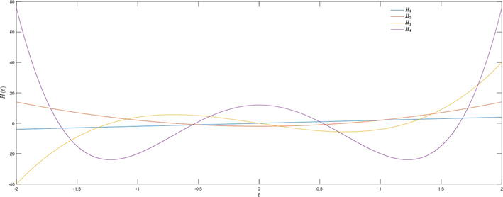
where the notation $⌊j⌋$ is the floor function that takes input as a real number $j$ and exhibits as output the greatest integer less than $j$. Using (10), one may compute the following HPs for $j=0,1,\cdots ,4$ as

$$H_j\left(t\right)=\left\{\begin{array}{ll}1,& \text{for}j=0,\\ 2t,& \text{for}j=1,\\ 4t^2-2,& \text{for}j=2,\\ 8t^3-12t,& \text{for}j=3,\\ 16t^4-48t^2+12,& \text{for}j=4.\end{array}\right.$$E11

The orthogonality conditions for HPs with respect to the weight function, $w\left(t\right)=\mathit{exp}\left(-t^2\right)$ are listed there

Figure 1.

Hermite polynomials plots for various $j$.

$${\int }_{-\infty }^{\infty }w\left(t\right)H_j\left(t\right)H_i\left(t\right)\mathrm{d}t=\left\{\begin{array}{ll}0,& \text{for}i\ne j,\\ \sqrt{\pi }{2}^j\mathrm{\Gamma }\left(j+1\right)& \text{for}i=j.\end{array}\right.$$E12

3.1 Useful properties of HPs

In this section, we list some interesting properties of HPs that are useful to construct integer-order derivative and integer-order integral operational matrices of HPs.

The following are the HPs recurrence relations, see [56].

$$H_j^{\left(1\right)}\left(t\right)=2{\mathit{jH}}_{j-1}\left(t\right),\text{for}j\ge 1.$$E13

$$H_{j+1}\left(t\right)=2{\mathit{tH}}_j\left(t\right)-2{\mathit{jH}}_{j-1}\left(t\right),\text{for}j\ge 1.$$E14

Any square-integrable function, i.e., $x\left(t\right)\in L^2\left(-\infty ,\infty \right)$ can be uniquely expressed as the basis of HPs in the following way

$$x\left(t\right)=\sum _{j=0}^{\infty }{h}_j{H}_j\left(t\right),$$E15

where $h_j$ are the series coefficients that can be computed using (12) as

$$h_j=\frac{1}{\sqrt{\pi }{2}^j\mathrm{\Gamma }\left(j+1\right)}{\int }_{-\infty }^{\infty }w\left(t\right)x\left(t\right)H_j\left(t\right)\mathrm{d}t,j=0,1,\cdots .$$E16

Considering the first $m+1$-terms of HPs, (15) can also be written as

$$x\left(t\right)\simeq \sum _{j=0}^m{h}_j{H}_j\left(t\right)={\chi }^T\mathrm{\Omega }\left(t\right),$$E17

where ${\chi }^T=\left[h_0,h_1,\cdots ,h_m\right]$ and $\mathrm{\Omega }\left(t\right)={\left[H_0\left(t\right),H_1\left(t\right),\cdots ,H_m\left(t\right)\right]}^T$.

4. Operational matrices of HPs

This section deals with the operational matrices of HPs that are constructed by using the analytical form (10) of HPs and Riemann–Liouville fractional-order integral operator and Hilfer fractional-order derivative operator.

Lemma 4.1. ([56], Section 3) The Hermite integer-order integral operational matrix can be determined by using the following integral property

$$\underset{k-\mathit{\text{times}}}{\underbrace{{\int }_0^t{\int }_0^t\cdots {\int }_0^t\mathrm{\Omega }\left(y\right){\left(\mathrm{d}y\right)}^k}}\simeq {\mathbf{P}}^k\mathrm{\Omega }\left(t\right),$$E18

where $\mathbf{P}$ is the $m+1\times m+1$ Hermite operational matrix of integration. For example, for $m=4$, and $k=1$, we have

$$\mathbf{P}=\left(\begin{array}{ccccc}0& \frac{1}{2}& 0& 0& 0\\ \frac{1}{2}& 0& \frac{1}{4}& 0& 0\\ 0& 0& 0& \frac{1}{6}& 0\\ -\frac{3}{2}& 0& 0& 0& \frac{1}{8}\\ 0& 0& 0& 0& 0\end{array}\right),$$E19

$$\mathrm{\Omega }\left(t\right)=\left(\begin{array}{c}1\\ 2t\\ 4t^2-2\\ 8t^3-12t\\ 16t^4-48t^2+12\end{array}\right),$$E20

and

$${\chi }^T=\left(\frac{1}{2}0\frac{1}{4}00\right).$$E21

Using (19)–(21), the approximate integral of $t^2$ is $\frac{t^3}{3}$ that coincides with the analytical integral of $t^2$.

Lemma 4.2. ([57], Thm. 1) The Hermite integer-order derivative operational matrix can be determined by using the following derivative property

$$\frac{d^k}{{\mathit{dt}}^k}\mathrm{\Omega }\left(t\right)={\left({\mathbf{H}}^{\left(1\right)}\right)}^k\mathrm{\Omega }\left(t\right),$$E22

where ${\mathbf{H}}^{\left(1\right)}$ is the $m+1\times m+1$ Hermite operational matrix of derivatives. Defined as.

$${\mathbf{H}}_{p,l}^{\left(1\right)}=\left\{\begin{array}{ll}2p,& \mathit{\text{for}}l=p-1,\\ 0,& \text{otherwise}.\end{array}\right.$$

For example at $m=5$, we have

$${\mathbf{H}}^{\left(1\right)}=\left(\begin{array}{cccccc}0& 0& 0& 0& 0& 0\\ 2& 0& 0& 0& 0& 0\\ 0& 4& 0& 0& 0& 0\\ 0& 0& 6& 0& 0& 0\\ 0& 0& 0& 8& 0& 0\\ 0& 0& 0& 0& 10& 0\end{array}\right),$$E23

$$\mathrm{\Omega }\left(t\right)=\left(\begin{array}{c}1\\ 2t\\ 4t^2-2\\ 8t^3-12t\\ 16t^4-48t^2+12\\ 32t^5-160t^3+120t\end{array}\right),$$E24

and

$${\chi }^T=\left(\begin{array}{cccccc}0.7788& -0.0000& -0.0974& 0.0000& 0.0020& 0.0000\end{array}\right).$$E25

Using (23)–(25), the approximate derivative of $cos\left(t\right)$ is as following

$$\frac{d}{\mathit{dt}}cos\left(t\right)\simeq 4t^4+0.12t^3-0.000000000000000022t^2-0.97t-0.000000000000000010.$$

Lemma 4.3. For $\gamma \in {\mathbb{R}}_{+}$ and $r,j\in \mathbb{N}$, we have the following result

$$\begin{array}{c}{t}^{j-2r+\gamma }\simeq \sum _{l=0}^m{d}_l{H}_l\left(t\right),\\ d_l=\frac{1}{2^{l}l!\sqrt{\pi }}\sum _{s=0}^{⌊\frac{l}{2}⌋}\frac{{\left(-1\right)}^{s}l!2^{l-2s}}{s!\left(l-2s\right)!}\times \mathrm{\Gamma }\left(\frac{l-2\left(s+r\right)+j+\gamma +1}{2}\right).\end{array}$$

Proof. Approximating $t^{j-2r+\gamma }$ by using the $m+1$-terms of HPs as

$$t^{j-2r+\gamma }\simeq \sum _{l=0}^m{d}_l{H}_l\left(t\right).$$E26

The series coefficients $d_l$ can be computed by using (16) as

$$\begin{array}{c}{d}_l=\frac{1}{2^{l}l!\sqrt{\pi }}{\int }_{-\infty }^{\infty }{t}^{j-2r+\gamma }{H}_l\left(t\right)w\left(t\right)\mathrm{d}t\\ =\frac{1}{2^{l}l!\sqrt{\pi }}\sum _{s=0}^{⌊\frac{l}{2}⌋}\frac{{\left(-1\right)}^{s}l!2^{l-2s}}{s!\left(l-2s\right)!}{\int }_{-\infty }^{\infty }{t}^{l-2\left(s+r\right)+j+\gamma }exp\left(-t^2\right)\mathrm{d}t.\end{array}$$E27

Using Lemma 2.3, we can write Eq. (27) as

$$d_l=\frac{1}{2^{l}l!\sqrt{\pi }}\sum _{s=0}^{⌊\frac{l}{2}⌋}\frac{{\left(-1\right)}^{s}l!2^{l-2s}}{s!\left(l-2s\right)!}\times \mathrm{\Gamma }\left(\frac{l-2\left(s+r\right)+j+\gamma +1}{2}\right).$$E28

Consequently, Eqs. (26) and (28) prove the result. □

Lemma 4.4. For $\alpha \in {\mathbb{R}}_{+}$ and $r,j\in \mathbb{N}$, we have the following result

$$\begin{array}{c}{t}^{j-2r-\alpha }\simeq \sum _{l=0}^m{f}_l{H}_l\left(t\right),\\ f_l=\frac{1}{2^{l}l!\sqrt{\pi }}\sum _{s=0}^{⌊\frac{l}{2}⌋}\frac{{\left(-1\right)}^{s}l!2^{l-2s}}{s!\left(l-2s\right)!}\times \mathrm{\Gamma }\left(\frac{l-2\left(s+r\right)+j-\alpha +1}{2}\right).\end{array}$$

Proof. Approximating $t^{j-2r-\alpha }$ by using the $m+1$-terms of HPs as

$$t^{j-2r-\alpha }\simeq \sum _{l=0}^m{f}_l{H}_l\left(t\right).$$E29

The series coefficients $f_l$ can be computed by using (16) as

$$\begin{array}{c}{f}_l=\frac{1}{2^{l}l!\sqrt{\pi }}{\int }_{-\infty }^{\infty }{t}^{j-2r-\alpha }{H}_l\left(t\right)w\left(t\right)\mathrm{d}t\\ =\frac{1}{2^{l}l!\sqrt{\pi }}\sum _{s=0}^{⌊\frac{l}{2}⌋}\frac{{\left(-1\right)}^{s}l!2^{l-2s}}{s!\left(l-2s\right)!}{\int }_{-\infty }^{\infty }{t}^{l-2\left(s+r\right)+j-\alpha }exp\left(-t^2\right)\mathrm{d}t.\end{array}$$E30

Using Lemma 2.3, we can write Eq. (30) as

$$f_l=\frac{1}{2^{l}l!\sqrt{\pi }}\sum _{s=0}^{⌊\frac{l}{2}⌋}\frac{{\left(-1\right)}^{s}l!2^{l-2s}}{s!\left(l-2s\right)!}\times \mathrm{\Gamma }\left(\frac{l-2\left(s+r\right)+j-\alpha +1}{2}\right).$$E31

Consequently, Eqs. (29) and (31) prove the result. □

4.1 New Hermite generalized operational matrices

In this section, we introduce new operational matrices of HPs that are used to approximate the derivative terms of the problem (1). The operational matrices are constructed in the senses of the Riemann–Liouville fractional-order integral operator and Hilfer fractional-order derivative operator.

Theorem 4.5. If $\mathrm{\Omega }\left(t\right)$ is the Hermite function vector as defined in Eq. (17), then

$${}_{\mathrm{RL}}{J}_{0^{+}}^{\gamma }\mathrm{\Omega }\left(t\right)\simeq {\mathbf{P}}^{\left(\gamma \right)}\mathrm{\Omega }\left(t\right),$$E32

where ${\mathbf{P}}^{\gamma }$ is the Hermite generalized integral operational matrix of order $\gamma \in {\mathbb{R}}_{+}$ and dimensions $m+1\times m+1$ that can be computed using the following expression

$${\mathbf{P}}^{\left(\gamma \right)}=\sum _{l=0}^m\left(\sum _{r=0}^{⌊\frac{j}{2}⌋}{\mathrm{\Psi }}_{j,l,r}\right),j=0,1,\cdots ,m,l=0,1,\cdots ,m,$$E33

where

$$\begin{array}{c}{\mathrm{\Psi }}_{\left(j,l,r\right)}=\sum _{s=0}^{⌊\frac{l}{2}⌋}\frac{{\left(-1\right)}^{r+s}j!l!2^{j-2r+l-2s}\mathrm{\Gamma }\left(\frac{l-2\left(s+r\right)+j+\gamma +1}{2}\right)}{r!s!\mathrm{\Gamma }\left(\gamma +j-2r+1\right)2^{l}l!\sqrt{\pi }\left(l-2s\right)!}.\end{array}$$E34

Proof. Applying the Riemann–Liouville fractional-order integral operator of order $\gamma \in {\mathbb{R}}_{+}$ defined in (5) to Eq. (10) and using (7), it yields

$${}_{\mathrm{RL}}{J}_{0^{+}}^{\gamma }{H}_j\left(t\right)=\sum _{r=0}^{⌊\frac{j}{2}⌋}\frac{{\left(-1\right)}^{r}j!2^{j-2r}\mathrm{\Gamma }\left(j-2r+1\right)}{r!\left(j-2r\right)!\mathrm{\Gamma }\left(j-2r+1+\gamma \right)}{t}^{j-2r+\gamma }.$$E35

The term $t^{j-2r+\gamma }$ can be approximated by using basis of HPs as

$$t^{j-2r+\gamma }\simeq \sum _{l=0}^m{d}_l{H}_l\left(t\right).$$E36

Using the result of Lemma 4.3, (36) can be written as

$$t^{j-2r+\gamma }=\sum _{l=0}^m\left(\frac{1}{2^{l}l!\sqrt{\pi }}\sum _{s=0}^{⌊\frac{l}{2}⌋}\frac{{\left(-1\right)}^{s}l!2^{l-2s}}{s!\left(l-2s\right)!}\times \mathrm{\Gamma }\left(\frac{l-2\left(s+r\right)+j+\gamma +1}{2}\right)\right)H_l\left(t\right).$$E37

Using Eq. (37) in Eq. (35), we have

$$\begin{array}{l}{}_{\mathrm{RL}}{J}_{0^{+}}^{\gamma }{H}_j\left(t\right)\simeq \sum _{r=0}^{⌊\frac{j}{2}⌋}\frac{{\left(-1\right)}^{r}j!2^{j-2r}\mathrm{\Gamma }\left(j-2r+1\right)}{r!\left(j-2r\right)!\mathrm{\Gamma }\left(j-2r+1+\gamma \right)}\times \\ \sum _{l=0}^m\left(\frac{1}{2^{l}l!\sqrt{\pi }}\sum _{s=0}^{⌊\frac{l}{2}⌋}\frac{{\left(-1\right)}^{s}l!2^{l-2s}}{s!\left(l-2s\right)!}\mathrm{\Gamma }\left(\frac{l-2\left(s+r\right)+j+\gamma +1}{2}\right)\right)H_l\left(t\right).\end{array}$$E38

After simplification, we can write (38) as

$$\begin{array}{c}{\mathrm{RL}}_{}{J}_{0^{+}}^{\gamma }{H}_j\left(t\right)\simeq \sum _{l=0}^m\left(\sum _{r=0}^{⌊\frac{j}{2}⌋}\sum _{s=0}^{⌊\frac{l}{2}⌋}\frac{{\left(-1\right)}^{r+s}j!l!2^{j-2r+l-2s}\mathrm{\Gamma }\left(\frac{l-2\left(s+r\right)+j+\gamma +1}{2}\right)}{r!s!\mathrm{\Gamma }\left(j-2r+\gamma +1\right)2^{l}l!\sqrt{\pi }\left(l-2s\right)!}\right)H_l\left(t\right)\\ =\sum _{l=0}^n\left(\sum _{r=0}^{⌊\frac{j}{2}⌋}{\mathrm{\Psi }}_{j,l,r}\right)H_l\left(t\right),j,l=0,1,\cdots ,m,\end{array}$$E39

where ${\mathrm{\Psi }}_{j,l,r}$ is given in (34). Now (39) in vector form can be written as

$${}_{\mathrm{RL}}{J}_{0^{+}}^{\gamma }{H}_j\left(t\right)\simeq \left[\sum _{r=0}^{⌊\frac{j}{2}⌋}{\mathrm{\Psi }}_{j,0,r},\sum _{r=0}^{⌊\frac{j}{2}⌋}{\mathrm{\Psi }}_{j,1,r},\sum _{r=0}^{⌊\frac{j}{2}⌋}{\mathrm{\Psi }}_{j,2,s}\cdots ,\sum _{r=0}^{⌊\frac{j}{2}⌋}{\mathrm{\Psi }}_{j,m,r}\right]\mathrm{\Omega }\left(t\right).$$E40

Consequently, the required result is proved. □

For example, at $j,l=0,1,\cdots ,3$ and $\gamma =3.5$, we have

$${\mathbf{P}}^{\left(3.5\right)}=\left(\begin{array}{cccc}0.0275& 0.0390& 0.0240& 0.0081\\ 0.0173& 0.0275& 0.0195& 0.0080\\ -0.0350& -0.0433& -0.0206& -0.0033\\ -0.0720& -0.1049& -0.0650& -0.0206\end{array}\right).$$

Theorem 4.6. If $\mathrm{\Omega }\left(t\right)$ is the Hermite function vector as defined in Eq. (17), then

$${}_{\mathrm{H}}{\mathcal{D}}_{0^{+}}^{\alpha ,\beta }\mathrm{\Omega }\left(t\right)\simeq {\mathbf{H}}^{\left(\alpha ,\beta \right)}\mathrm{\Omega }\left(t\right),$$E41

where ${\mathbf{H}}^{\alpha ,\beta }$ is the Hermite generalized derivative operational matrix of order $\alpha$ and dimensions $m+1\times m+1$ that can be computed using the following expression

$${\mathbf{H}}^{\left(\alpha ,\beta \right)}=\sum _{l=0}^m\left(\sum _{r=0}^{⌊\frac{j-⌈\alpha ⌉}{2}⌋}{\mathrm{\Phi }}_{j,l,r}\right),j=⌈\alpha ⌉,\cdots ,m,l=0,1,\cdots ,m,$$E42

where

$$\begin{array}{c}{\mathrm{\Phi }}_{\left(j,l,r\right)}=\sum _{s=0}^{⌊\frac{l}{2}⌋}\frac{{\left(-1\right)}^{r+s}j!l!2^{j-2r+l-2s}\mathrm{\Gamma }\left(\frac{l-2\left(s+r\right)+j-\alpha +1}{2}\right)}{r!s!\mathrm{\Gamma }\left(j-2r+1-\alpha \right)2^{l}l!\sqrt{\pi }\left(l-2s\right)!}.\end{array}$$E43

Proof. Applying the Hilfer fractional-order derivative operator of order $\alpha$ defined in Definition (1) to Eq. (10) and using Lemma 2.2, it yields

$${}_{\mathrm{H}}{\mathcal{D}}_{0^{+}}^{\alpha ,\beta }{H}_j\left(t\right)=\sum _{r=0}^{⌊\frac{j-⌈\alpha ⌉}{2}⌋}\frac{{\left(-1\right)}^{r}j!2^{j-2r}\mathrm{\Gamma }\left(j-2r+1\right)}{r!\left(j-2r\right)!\mathrm{\Gamma }\left(j-2r+1-\alpha \right)}{t}^{j-2r-\alpha },j=⌈\alpha ⌉,⌈\alpha ⌉+1,\cdots ,m.$$E44

The term $t^{j-2r-\alpha }$ can be approximated by using basis of HPs as

$$t^{j-2r-\alpha }\simeq \sum _{l=0}^m{f}_l{H}_l\left(t\right).$$E45

Using the result of Lemma 4.4, Eq. (45) can be written as

$$t^{j-2r-\alpha }=\sum _{l=0}^m\left(\frac{1}{2^{l}l!\sqrt{\pi }}\sum _{s=0}^{⌊\frac{l}{2}⌋}\frac{{\left(-1\right)}^{s}l!2^{l-2s}}{s!\left(l-2s\right)!}\times \mathrm{\Gamma }\left(\frac{l-2\left(s+r\right)+j-\alpha +1}{2}\right)\right)H_l\left(t\right).$$E46

Using Eq. (46) in Eq. (44), we have

$$\begin{array}{l}{}_{\mathrm{H}}{\mathcal{D}}_{0^{+}}^{\alpha ,\beta }{H}_j\left(t\right)\simeq \sum _{r=0}^{⌊\frac{j-⌈\alpha ⌉}{2}⌋}\frac{{\left(-1\right)}^{r}j!2^{j-2r}\mathrm{\Gamma }\left(j-2r+1\right)}{r!\left(j-2r\right)!\mathrm{\Gamma }\left(j-2r+1-\alpha \right)}\times \\ \sum _{l=0}^m\left(\frac{1}{2^{l}l!\sqrt{\pi }}\sum _{s=0}^{⌊\frac{l}{2}⌋}\frac{{\left(-1\right)}^{s}l!2^{l-2s}}{s!\left(l-2s\right)!}\mathrm{\Gamma }\left(\frac{l-2\left(s+r\right)+j-\alpha +1}{2}\right)\right)H_l\left(t\right).\end{array}$$E47

After simplification, we can write (47) as

$$\begin{array}{c}{\mathrm{H}}_{}{\mathcal{D}}_{0^{+}}^{\alpha ,\beta }{H}_j\left(t\right)\simeq \sum _{l=0}^m\left(\sum _{r=0}^{⌊\frac{j-⌈\alpha ⌉}{2}⌋}\sum _{s=0}^{⌊\frac{l}{2}⌋}\frac{{\left(-1\right)}^{r+s}j!l!2^{j-2r+l-2s}\mathrm{\Gamma }\left(\frac{l-2\left(s+r\right)+j-\alpha +1}{2}\right)}{r!s!\mathrm{\Gamma }\left(j-2r-\alpha +1\right)2^{l}l!\sqrt{\pi }\left(l-2s\right)!}\right)H_l\left(t\right)\\ =\sum _{l=0}^m\left(\sum _{r=0}^{⌊\frac{j-⌈\alpha ⌉}{2}⌋}{\mathrm{\Phi }}_{j,l,r}\right)H_l\left(t\right),j=⌈\alpha ⌉,\cdots ,m,l=0,1,\cdots ,m,\end{array}$$E48

where ${\mathrm{\Phi }}_{j,l,r}$ is given in (43). Now (48) in vector form can be written as

$${}_{\mathrm{H}}{\mathcal{D}}_{0^{+}}^{\alpha ,\beta }{H}_j\left(t\right)\simeq \left[\sum _{r=0}^{⌊\frac{j-⌈\alpha ⌉}{2}⌋}{\mathrm{\Phi }}_{j,0,r},\sum _{r=0}^{⌊\frac{j-⌈\alpha ⌉}{2}⌋}{\mathrm{\Phi }}_{j,1,r},\sum _{r=0}^{⌊\frac{j-⌈\alpha ⌉}{2}⌋}{\mathrm{\Phi }}_{j,2,s}\cdots ,\sum _{r=0}^{⌊\frac{j-⌈\alpha ⌉}{2}⌋}{\mathrm{\Phi }}_{j,m,r}\right]\mathrm{\Omega }\left(t\right).$$E49

Consequently, the required result is proved. □

For example, at $j,l=0,1,\cdots ,3$, $\alpha =1.5$, and $\beta =1$, we have

$${\mathbf{H}}^{\left(\mathrm{1.5,1}\right)}=\left(\begin{array}{cccc}0& 0& 0& 0\\ 0& 0& 0& 0\\ 3.1205& 2.3081& 0.3901& -0.0962\\ 9.2325& 9.3615& 3.4622& 0.3901\end{array}\right).$$

5. Applications of Hermite operational matrices

In this section, we develop a numerical algorithm that is based on the Hermite integrals and derivatives operational matrices. The framework of the proposed algorithm transforms the problem (1) to matrix equations of Sylvester types that are easy to handle with any computational software. The matrix equations compute the unknown vector ${\chi }^T$ which leads to the solution of the problem (1).

Suppose the following holds true

$${}_{\mathrm{H}}{\mathcal{D}}^{\alpha ,\beta }x\left(t\right)={\chi }^T\mathrm{\Omega }\left(t\right).$$E50

Integrating the Eq. (50) by applying the Riemann–Liouville fractional-order integral defined in (5) of order $\gamma$, we have

$$x\left(t\right)={\chi }_{\mathrm{RL}}^T{J}^{\gamma }\mathrm{\Omega }\left(t\right)+\sum _{a=0}^1{b}_a{t}^a,1<\gamma \le 2,0<\beta \le 1,$$E51

where $b_a$’s are the constant of integration determined by using the initial conditions (1), we have the following equation

$$x\left(t\right)={\chi }_{\mathrm{RL}}^T{J}^{\gamma }\mathrm{\Omega }\left(t\right)+\sum _{a=0}^1{c}_a{t}^a.$$E52

Using Theorem 4.5 and approximating the term ${\sum }_{a=0}^1{c}_a{t}^a$ with Hermite function vector, Eq. (51) can also be expressed as

$$x\left(t\right)\simeq {\chi }^T{\mathbf{P}}^{\left(\gamma \right)}\mathrm{\Omega }\left(t\right)+B_{\left(1\times m+1\right)}^T\mathrm{\Omega }\left(t\right),$$E53

where ${\sum }_{a=0}^1{c}_a{t}^a=B_{\left(1\times m+1\right)}^T\mathrm{\Omega }\left(t\right)$. The terms of the problem (1) can be computed by using Theorem 4.6 and Eq. (53), we have

$$\left\{\begin{array}{l}{}_{\mathrm{H}}{\mathcal{D}}^{\alpha ,\beta }x\left(t\right)={\chi }^T{\mathbf{P}}^{\left(\gamma \right)}{\mathbf{H}}^{\left(\alpha ,\beta \right)}\mathrm{\Omega }\left(t\right)+B_{\left(1\times m+1\right)}^T{\mathbf{H}}^{\left(\alpha ,\beta \right)}\mathrm{\Omega }\left(t\right),\\ y\left(t\right)=A_{\left(1\times m+1\right)}^T\mathrm{\Omega }\left(t\right).\end{array}\right.$$E54

Using Eqs. (50), (53), and (54) in (1), we have the following matrix equation of Sylvester type with an unknown vector ${\chi }^T$ of dimensions $1\times m+1$.

$$\begin{array}{c}{\chi }^T\mathrm{\Omega }\left(t\right)+{\chi }^T\left({\lambda }_1{\mathbf{P}}^{\left(\gamma \right)}{\mathbf{H}}^{\left(\alpha ,\beta \right)}+{\lambda }_2{\mathbf{P}}^{\left(\gamma \right)}\right)\mathrm{\Omega }\left(t\right)=\left(A_{\left(1\times m+1\right)}^T-{\lambda }_1{B}_{\left(1\times m+1\right)}^T{\mathbf{H}}^{\left(\alpha ,\beta \right)}-{\lambda }_2{B}_{\left(1\times m+1\right)}^T\right)\mathrm{\Omega }\left(t\right)\end{array}$$E55

By introducing the notations, ${\mathrm{\Delta }}_{\left(m+1\times m+1\right)}={\lambda }_1{\mathbf{P}}^{\left(\gamma \right)}{\mathbf{H}}^{\left(\alpha ,\beta \right)}+{\lambda }_2{\mathbf{P}}^{\left(\gamma \right)}$ and ${\mathrm{\Lambda }}_{\left(1\times m+1\right)}=A_{\left(1\times m+1\right)}^T-{\lambda }_1{B}_{\left(1\times m+1\right)}^T{\mathbf{H}}^{\left(\alpha ,\beta \right)}-{\lambda }_2{B}_{\left(1\times m+1\right)}^T$ for the sake of simplifications, Eq. (55) can be written as

$${\chi }_{\left(1\times m+1\right)}^T+{\chi }_{\left(1\times m+1\right)}^T{\mathrm{\Delta }}_{\left(m+1\times n+1\right)}={\mathrm{\Lambda }}_{\left(1\times m+1\right)}.$$E56

By solving (56), we can easily compute the unknown vector ${\chi }_{\left(1\times m+1\right)}^T$ which then substituting in Eq. (53) yields the solution of the problem (1).

6. Examples

In this section, we solve some examples to test the applicability and efficiency of the proposed algorithm discussed in Section 5. The results are displayed in Tables and Plots.

Example 6.1. Consider the following Bagley–Torvik equation with initial conditions

$$\begin{array}{l}{\lambda }_3{x^{\prime }}^{\prime }\left(t\right)+{\lambda }_{1\mathrm{H}}{\mathcal{D}}^{\alpha ,\beta }x\left(t\right)+{\lambda }_{2}x\left(t\right)=y\left(t\right),t\in \left(-10,10\right),\\ x\left(0\right)=c_1,x^{\prime }\left(0\right)=c_2,\end{array}$$E57

where, $y\left(t\right)=1+t$, $1<\alpha <2$, $0<\beta <1$, $c_1=0$, $c_2=1$, and ${\lambda }_1={\lambda }_2={\lambda }_3=1$.

At $m=2$, we

$${\mathbf{P}}^{\left(2\right)}=\left(\begin{array}{ccc}\frac{1}{8}& \frac{5081767996463981}{36028797018963968}& \frac{1}{16}\\ \frac{6775690661951975}{72057594037927936}& \frac{1}{8}& \frac{5081767996463981}{72057594037927936}\\ -\frac{1}{8}& -\frac{6775690661951975}{72057594037927936}& 0\end{array}\right),$$E58

$${\mathbf{H}}^{\left(\mathrm{1.5,1}\right)}=\left(\begin{array}{ccc}0& 0& 0\\ 0& 0& 0\\ \frac{7026736834630197}{2251799813685248}& \frac{5197457860426675}{2251799813685248}& \frac{7026736834630197}{18014398509481984}\end{array}\right),$$E59

$${\chi }^T=\left(\begin{array}{ccc}-\frac{1917597440026193}{2596148429267413814265248164610048}& -\frac{5162427874821681}{10384593717069655257060992658440192}& -\frac{734167200735167}{81129638414606681695789005144064}\end{array}\right),$$E60

$$\mathrm{\Omega }\left(t\right)=\left(\begin{array}{c}1\\ 2t\\ 4t^2-2\end{array}\right).$$E61

Using Eqs. (58)–(61), the approximated solution, $\widehat{x\left(t\right)}$ of the Example 6.1 is $1+t$, which coincides with its exact solution, $x\left(t\right)=1+t$ at $\alpha =\frac{3}{2}$ and $\beta =1$.

Example 6.2. Consider the following Bagley–Torvik equation with initial conditions

$$\begin{array}{l}{\lambda }_3{x^{\prime }}^{\prime }\left(t\right)+{\lambda }_{1e\mathrm{H}}{\mathcal{D}}^{\alpha ,\beta }x\left(t\right)+{\lambda }_{2}x\left(t\right)=y\left(t\right),t\in \left(-2,2\right),\\ x\left(0\right)=c_1,x^{\prime }\left(0\right)=c_2,\end{array}$$E62

where, $y\left(t\right)={\lambda }_2\left(1+t\right)$, $1<\alpha <2$, $0<\beta <1$, $c_1=0$, $c_2=1$, ${\lambda }_1=1.5$, ${\lambda }_2=2.5$, and ${\lambda }_3=1$.

Example 6.3. Consider the following Bagley–Torvik equation with initial conditions

$$\begin{array}{l}{\lambda }_3{x^{\prime }}^{\prime }\left(t\right)+{\lambda }_{1\mathrm{H}}{\mathcal{D}}^{\alpha ,\beta }x\left(t\right)+{\lambda }_{2}x\left(t\right)=y\left(t\right),t\in \left(0,1\right),\\ x\left(0\right)=c_1,x^{\prime }\left(0\right)=c_2,\end{array}$$E63

where, $y\left(t\right)=8$, $1<\alpha <2$, $0<\beta <1$, $c_1=0=c_2$, ${\lambda }_3=1$, and ${\lambda }_1=0.5={\lambda }_2$. The analytical solution of Example 6.3 is given as

$$x\left(t\right)={\int }_0^{t}G\left(t-z\right)y\left(z\right)\mathit{dz},$$E64

where $G$ is a Green function given as under

$$G\left(t\right)=\sum _{l=0}^{\infty }\frac{{\left(-1\right)}^l}{\mathrm{\Gamma }\left(l+1\right)}{\lambda }_2^l{t}^{2l+1}{E}_{1/2,2+3l/2}^{\left(l\right)}\left(-{\lambda }_1\sqrt{t}\right),$$E65

The expression $E_{\gamma ,\delta }^{\left(l\right)}$ is the $\mathit{lth}$ derivative of the two parametric Mittagg-Leffler function, given as ([26], (8.26))

$$E_{\gamma ,\delta }^{\left(l\right)}\left(t\right)=\sum _{i=0}^{\infty }\frac{\mathrm{\Gamma }\left(i+l+1\right)t^i}{\mathrm{\Gamma }\left(i+1\right)\mathrm{\Gamma }\left(\mathit{\gamma i}+\mathit{\gamma l}+\delta \right)},l=0,1,\cdots .$$E66

Example 6.4. Consider the following Bagley–Torvik equation with initial conditions

$$\begin{array}{l}{\lambda }_3{x}^{\left(\gamma \right)}\left(t\right)+{\lambda }_{1\mathrm{H}}{\mathcal{D}}^{\alpha ,\beta }x\left(t\right)+{\lambda }_{2}x\left(t\right)=y\left(t\right),t\in \left(0,2\right),\\ x\left(0\right)=c_1,x^{\prime }\left(0\right)=c_2\end{array}$$E67

where, $y\left(t\right)=0$, $0<\gamma <2$, $c_1=1$, $c_2=0$, ${\lambda }_3=1$, ${\lambda }_1=0$, and ${\lambda }_2=1$. The exact solution of Example 6.4 at $\gamma =2$ is, $x\left(t\right)=cos\left(t\right)$.

7. Discussion

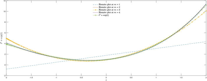
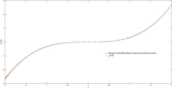
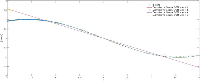
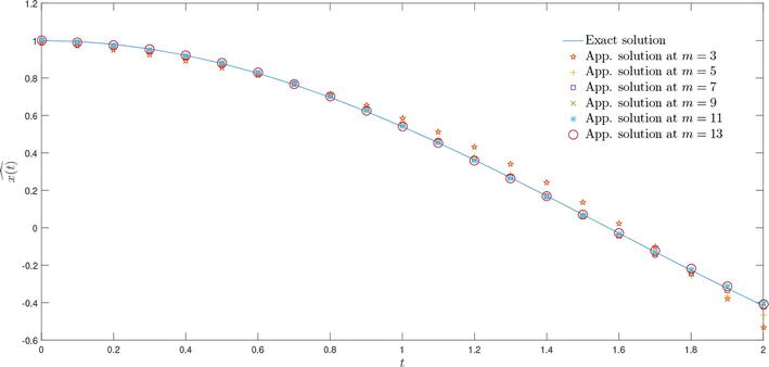
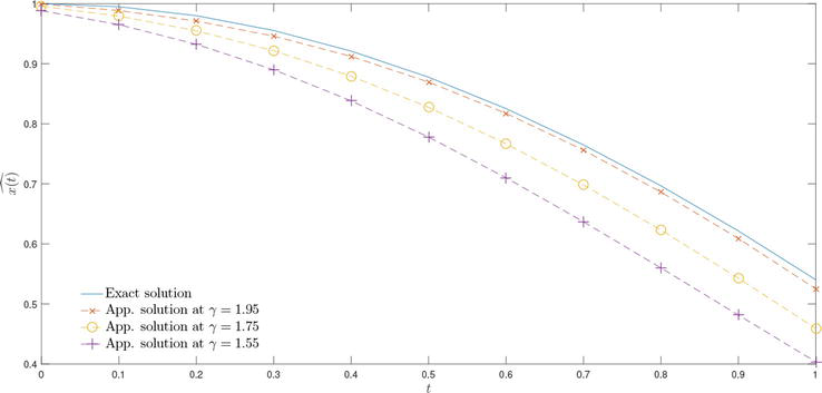
We solved the Bagley–Torvik FDDE by developing the fractional-order derivative operational matrices of HPs. The operational matrices were developed in the sense of Hilfer fractional-order derivative. We observed that HPs’ basis is well fit to approximate any square-integrable function on the entire real line, see Figures 1 and 2. Also, the integrals and derivatives of square-integrable functions were computed by using the Hermite operational matrices had a great resemblance with the results computed by using the analytical techniques of integrals and derivatives, see Figures 3 and 4. Based on the Hermite operational matrices, we introduced a numerical algorithm that is capable to transform the FDDE into a system of matrix equations of Sylvester types that are easy to handle with any computational software. We checked the accuracy and stability of the PNA by solving various Bagley–Torvic types FDDE corresponding to various initial conditions. We observed that the approximate solution obtained by using the PNA coincided with the exact solution by taking only a few terms of HPs, see (Example 6.1, Figure 5) and (Example 6.2, Table 1). We also analyzed the stability of the PNA by computing the approximate solution at various values of $\alpha$ and at various values of $m$, see Figures 6–10, and Table 2. We noted that as $m$ getting large and $\alpha$ was getting closer to $\frac{3}{2}$, the approximate solution approached to the exact solution of the problem. We also computed the amount of the absolute error for Example 6.4 at various values of $m$, and observed that the error decreased significantly for increasing $m$, see Table 3. The numerical accuracy of the results computed by using PNA was also analyzed by comparing the results with the Adomian method. We noted that the PNA prodoced better accuracy as compared to the Adomian method, see (Example 6.3, Table 2).

Figure 2.

Approximation of $t^2+exp\left(t\right)$ using Hermite function vectors (17) at various values of $m$.

Figure 3.

The analytical and approximate integral plots of $t^2$ at $m=4$ by using Hermite integral operational matrix.

Figure 4.

The analytical and approximate derivative plots of $cos\left(t\right)$ at different values of $m$ by using Hermite derivative operational matrices (DOM).

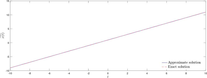
Figure 5.

The graphical view of exact and approximate solutions of Example 6.1 at $m=2$, and $\alpha =1.5$.

$t$	$\widehat{x\left(t\right)}$ at $m=2$	$\widehat{x\left(t\right)}$ at $m=3$	$\widehat{x\left(t\right)}$ at $m=10$	$\widehat{x\left(t\right)}$ at $m=15$	Exact solution
−1	0.0	0.0	0.0	0.0	0.0
−0.8	0.2	0.2	0.2	0.2	0.2
−0.6	0.4	0.4	0.4	0.4	0.4
−0.4	0.6	0.6	0.6	0.6	0.6
−0.2	0.8	0.8	0.8	0.8	0.8
0	1.0	1.0	1.0	1.0	1.0
0.2	1.2	1.2	1.2	1.2	1.2
0.4	1.4	1.4	1.4	1.4	1.4
0.6	1.6	1.6	1.6	1.6	1.6
0.8	1.8	1.8	1.8	1.8	1.8
1	2.0	2.0	2.0	2.0	2.0

Table 1.

Approximate solution of Example 6.2 is computed at various $m$.

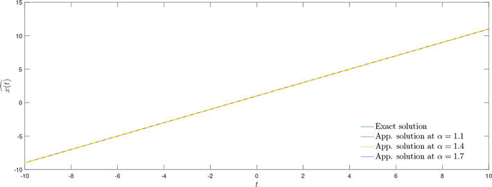
Figure 6.

The graphical view of exact and approximate solutions of Example 6.1 at $m=2$, and various values of $\alpha$.

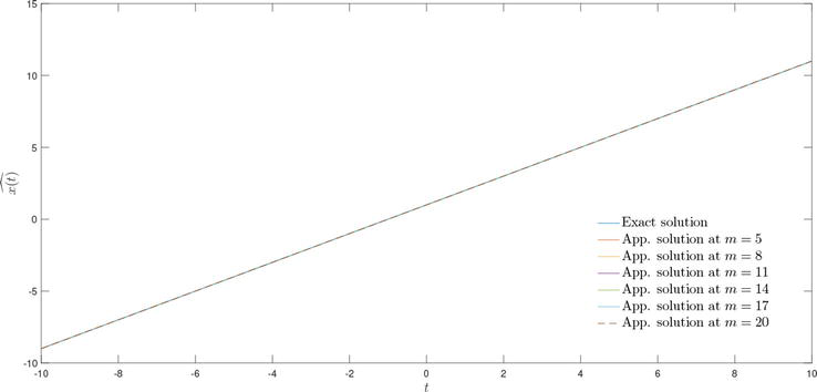
Figure 7.

The graphical view of exact and approximate solutions of Example 6.1 at $\alpha =1.5$, and various values of $m$.

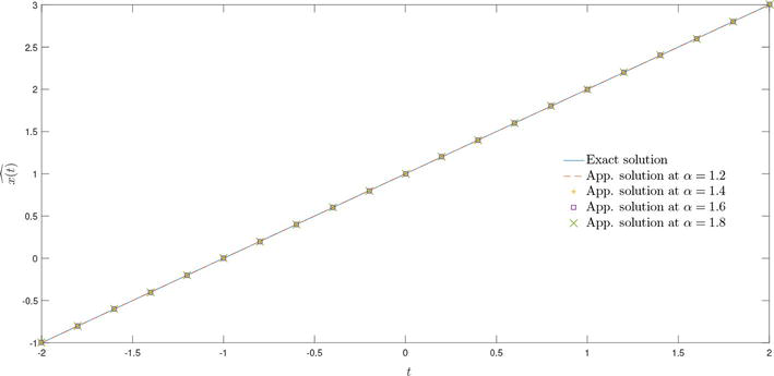
Figure 8.

The graphical view of exact and approximate solutions of Example 6.2 at $m=2$, and various values of $\alpha$.

Figure 9.

The graphical view of exact and approximate solutions of Example 6.4 at various values of $m$.

Figure 10.

The graphical view of exact and approximate solutions of Example 6.4 at $m=12$, and various values of $\gamma$.

$t$	Analytical solution	Adomian method	PNA at $m=16$	PNA at $m=20$
0	0.000000	0.000000	0.000000	0.000000
0.2	0.125221	0.140640	0.168975	0.147779
0.4	0.455435	0.533284	0.509874	0.491041
0.6	0.950392	1.148840	1.0384000	1.024804
0.8	1.579557	1.963033	1.726857	1.693681
1	2.315526	2.952567	2.524754	2.453043

Table 2.

Approximate solution of Example 6.3 obtained using the proposed numerical algorithm (PNA) are compared with the solution obtained using the Adomian method [32].

$t$	Error at $m=5$	Error at $m=7$	Error at $m=9$	Error at $m=15$	Error at $m=30$
0	0.000851555699954	0.000015168258275	0.000038589837968	0.000011170515838	0.000000771779988
0.2	0.013708145743312	0.009294768239541	0.007147462915103	0.003988632129512	0.000055034808212
0.4	0.011893816308316	0.006240104002812	0.003411075508628	0.000010952382595	0.000000030115944
0.6	0.001779738199402	0.001752762045013	0.003127688012188	0.003162961831284	0.000009796683838
0.8	0.010343264247858	0.008577085429824	0.006809926671596	0.002261792740019	0.000000600336283
1	0.018882601807647	0.010311814708410	0.005334232561979	0.000946037042348	0.000000892574348

Table 3.

Absolute error of Example 6.4 is computed at various $m$.

Classification

2020 Mathematics Subject Classification. 65 L05, 26A33, 35R11