Small Area Estimation for Demographic Analysis

Abstract

In this chapter we will introduce recent developments in the application of small area estimation (SAE) such as combining new statistical methods, e.g., multilevel regression and poststratification (MRP) and neighborhood spatial smoothing models (e.g., a modified Besag-York-Mollié, or BYM2), and consider recent applications for demographic processes such as mortality or migration estimation at local levels. We will discuss recent methodological developments and important applications of SAE such as the United Nations COVID-19 national and subnational mortality estimates. Last, we will provide a clear example of SAE using United States ZIP code-level data for core demographic questions relating to mortality and migration.

1. Introduction

Demography is a discipline dependent on the accurate enumeration of population-level processes. The foundational unit of measurement for analyzing many demographic processes is the count of individuals; it allows demographers to derive all other statistical descriptions of population dynamics. Therefore, it is crucial to have reliable population counts of the outcome of interest whether they relate to mortality (e.g., number in the population who died), fertility (e.g., number of births in the population), morbidity (e.g., number who contracted a disease), population-level social attitudes (e.g., measurable responses to a sociological survey), migration (e.g., counts of movement between locations), or otherwise. Unless there is near-perfect enumeration through a census, it is often difficult to establish the count of an outcome in a population. Classic survey methods and modern statistics offer a way to directly estimate these counts. However, when a survey has inadequate sample size, it may not be possible to make reliable direct estimates of the outcome of interest (e.g., counts of people 5–10 years old in Nigeria). Instead, it is often possible to make indirect estimates through methods that are often referred to as small area estimation (SAE). Here, a small area may either refer geographic areas/regions (e.g., counties, states, provinces, census tracts, etc.) or demographic groups (i.e., the various combinations of demographic characteristics present in survey data used to categorize individual participants, including sex, age, race/ethnicity, employment status, etc.) [1]. Small area estimation methods use additional contextual information to produce statistically robust estimates of under- or unobserved subpopulations or geographic units. Classic spatial models used for public health mapping and small area estimation include the Fay-Herriot model [2], the Besag-York-Mollié model [3], and the modified Besag-York-Mollié model (referred to as the BYM2 model) [4]. While SAE may use such spatial models in producing estimates, recent advancements in computational power mean that in many cases these models are only just beginning to be considered as potentially viable additions to more common SAE methods like multilevel regression and poststratification.

2. Small area estimation in demographic research

The building blocks of demographic research are census and survey data. As discussed, sometimes these data are unreliable, incomplete, or not measured in a timely manner. Increasingly, demographers are using SAE methods to attempt to produce more reliable indirect estimates as part of their analytic processes. This is especially true in high- and middle-income countries where data sparseness may exist in some geographic regions or demographic domains, but data quality and presence are otherwise high. While direct methods of SAE may incorporate estimation needs into survey designs, it is frequently also the case that post-hoc SAE is necessary using data not gathered explicitly for the purpose of generating estimates of the outcome of interest. In this case, indirect estimates may be produced using SAE methods applied to either census or survey data.

2.1 Small area estimation and census data

Many census authorities and national statistics offices have begun to use SAE for minor applications focused on tracking population trends during inter-census periods among subpopulations that are difficult to enumerate or underrepresented in inter-census data. For example, the United States Census Bureau has several small projects aimed at incorporating both geographic and temporal SAE methods to generate estimates in response to data user demands for increasingly finer-grain geographic areas like census tracts when complete domain data and/or adequate sample size are not available [5]. The American Community Survey (ACS) is perhaps the most well-known United States-based project that uses SAE methods; every month the ACS samples select households in all counties and produces model-based direct estimates of many outcomes of interest. A significant product of the ACS is indirect estimates of the number of school-aged children living in poverty at the county and school district levels which are published in yearly and five-year aggregates, as are all other ACS estimates. At such a fine-grain geographic level it may be difficult and invasive to directly enumerate the number of children experiencing poverty, but SAE methods allow the researcher to leverage sub-population level demographic data from sampled households to produce indirect estimates in a reasonably unobtrusive yet reliable manner. Similar work has been undertaken to produce indirect estimates for public health surveillance, including estimating disease prevalence such as with cancer cases [6], and health insurance coverage [7].

2.2 Small area estimation and non-census survey data

Just as with census authority work, a survey design or model may be produced to best represent attitudes by demographic characteristics and geographic context of any number of questions from opinion survey responses. In this context, SAE methods may then be used by organizations or groups interested in attitudes or opinions such as in academic contexts (e.g., sociologists, anthropologists, etc.), or business (e.g., market research). While classic use cases regarding public opinion polls are referenced below, some interesting and unique examples of these include estimating forest land ownership for the United States Department of Agriculture National Forest Service [8] and Australian electoral district-level attitudes toward same-sex marriage [9]. However, with these examples there is a presumption of high-quality data and limited “missingness” in terms of even fine-grain geographic coverage. In countries that may have fewer or limited resources for adequate enumeration efforts through a formal census (often low-income countries), additional information may be generated from observed population data using SAE. For example, the UNICEF Under 5 Year Mortality Estimates are a series of regularly produced estimates of small area mortality rates that use national census and survey data, and complex SAE methods for countries of particular concern regarding child survival rates [10]. In this way, SAE offers estimation methods of varying complexity and with varying thresholds of statistical expertise required for implementation but is also a suite of methods that can be applied flexibly to various population enumeration needs given data availability and adequate consideration. However, one SAE method that can be implemented with an accessible threshold level of expertise and is increasingly popular in high- and middle-income contexts is multilevel regression and poststratification.

3. Multilevel regression and poststratification: a basic introduction

Multilevel regression and poststratification (MRP) is a model-based statistical method that uses national/high-level administrative survey or census data¹ to adjust for non-representativeness in subnational surveys using national survey or census estimates, and/or to provide small area estimation (SAE) in areas where subnational survey data are sparse or nonexistent. MRP is computationally inexpensive and able to yield quick, consistent, and accurate estimates. Consequently, it is used for resource allocation and policy planning in settings such as public health administration. Prevailing methods of MRP for SAE borrow strength from other administrative areal data through partial pooling. While this approach is powerful, it does not account for any potential existing “neighborhood” spatial structure in the data. Including spatial specifications in MRP can be a valuable way to better handle spatial relationships and generate more accurate area-level estimates.

3.1 Traditional multilevel-regression and poststratification

The traditional MRP method described initially by Gelman and Little [11], and later expanded upon to consider applications for public opinion polls and surveys (e.g., [11, 12]; see also: [13, 14, 15]), is able to estimate the joint posterior distributions of the outcome of interest according to the survey population structure, and using Bayesian methods² to generate marginal estimates for unobserved subpopulations. It then adjusts these distributions using census or large-scale weighted population survey data to reflect the known population structure. If desired, it is then possible to use the mean posterior estimate (i.e., Bayesian methods) for each subpopulation in addition to the known area-level subpopulation counts from the same census data to predict the number of individuals in each area exhibiting the outcome of interest (the outcome is often assumed to have a binomial distribution, but this is not strictly required).

3.2 Data requirements for model fitting and poststratification

While a relatively straightforward procedure (described more thoroughly below), MRP has strict data requirements. Typically, the multilevel regression model built must only use as covariates the variables present in both the survey data used to train the model, and also the census data used to poststratify the marginal posterior probabilities. These complementary variables must be organized and coded in the exact same way (e.g., if “age” is used as a covariate, then each dataset must either represent age as a continuous variable, or bin age groups in the same manner). The individual-level survey data should contain at minimum two demographic characteristics per observed participant, in addition to good data availability for the outcome of interest to be modeled. For example, in addition to the respondent’s reported value for the outcome of interest, the sex and age; or sex and race/ethnicity; or sex, age and race/ethnicity must be known for each participant, and these characteristics must also be present in the census data. More concretely, if a model is built with the survey data using sex, age and race/ethnicity as the model covariates on which to later poststratify with the census data, then the census data must contain the known number of individuals belonging to each combination of covariate characteristics even if that number is zero (e.g., the number of people in the state of California who are identified as Black, male and aged 18–24; or the number of people in King County, Washington, USA, who are identified as White, female, and aged 25–34, etc., and every possible combination of these demographic characteristics). To this end, there must be a poststratification table that contains only the variables from the census data used to weight the joint posterior estimates and derive an estimated population count of the outcome. Furthermore, to adjust the estimates using the census data contained in the original poststratification table, it is necessary to calculate the inclusion weights of each poststratification level (e.g., the number of individuals in the poststratification level in ZIP code X divided by the total number of individuals in all poststratification levels in ZIP code X; these levels are clarified below).

3.3 Traditional MRP versus MRP using spatial specifications

For the multilevel model aspect of the MRP method, covariates are typically either modeled as fixed effects or random effects and may include interaction terms between fixed effects. The model is also where the traditional MRP method differs from MRP using spatial specifications. Traditional MRP methods may specify a hierarchical model of the probability of some outcome (which can then be extrapolated to estimate the count of individuals exhibiting the outcome in the population) as follows. Imagine we are estimating an outcome within the adult population (18 years and older) of a state, such as California, USA, and we have access to individual-level information about the outcome of interest within the California population; specifically the survey respondents’ ages and their county of residence. Define $N_{\mathit{ij}}$ as the population in age strata j = 1,…7 (where 1 = 18–24 years, 2 = 25–34 years, 3 = 35–44 years, 4 = 45–54 years, 5 = 55–64 years, 6 = 65–74 years, and 7 = 75 years and over) within each county i = 1,…58 (there are 58 counties in this state). The total population in each county in the state of California is $N_i={\sum }_{j=1}^J{N}_{\mathit{ij}}$, whereas the total population in the state of California is $N={\sum }_{i=1}^I{\sum }_{j=1}^J{N}_{\mathit{ij}}$. Let $y_{\mathit{ij}}$ be the number of people who exhibited the outcome out of the total $N_{\mathit{ij}}$ people in county i and age strata J, with $p_{\mathit{ij}}$ the probability of the outcome. We specify the hierarchical model,

$$y_{\mathit{ij}}\mid p_{\mathit{ij}}~\mathit{\text{Binomial}}\left(N_{\mathit{ij}},p_{\mathit{ij}}\right),$$E1

$$\mathit{log}\mathit{it}\left(p_{\mathit{ij}}\right)=\alpha +{\beta }_j+e_i,$$E2

$$\underset{\_}{\beta }=\left[{\beta }_1,\cdots {\beta }_J\right]~\mathit{RW}2\left({\sigma }_{\beta }^2\right),$$E3

$$e_i~\mathit{iid}N\left(0,{\sigma }_e^2\right),$$E4

and α the intercept (to include an intercept, the RW2 model requires a sum-to-zero constraint for identifiability). Here, RW2 is a random walk of the second order on age (perhaps an optimistic assumption with so few age categories, but a good example of a structured random effect one might use in these contexts). In this form, it is possible to specify the geographic area covariate as a random effect for partial local pooling within the context of each of the areas between different categories within a demographic variable (e.g., partial pooling within ZIP code X within different categories of race/ethnicity), but this formulation does not account for spatial structure (i.e., the model does not specify a “neighborhood” spatial structure, and there is no sharing between geographic areas contingent on proximity).

It is possible to use spatial terms in the model if the survey data contain any spatial information also identifiable in the census data (e.g., if the geographic area level of interest is the county level in the context of the United States, these would be United States Census Bureau county FIPS codes which represent each individual county and for which a spatial polygon/shapefile may be easily obtained). While covariates in the model in the traditional MRP method are specified as being independent and identically distributed (IID), the flexible nature of multilevel models can be leveraged such that a spatial random effect may be included in the model (after [16]).

3.3.1 Spatial specifications and poststratification data needs

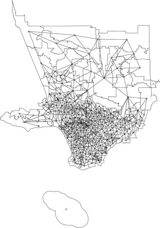
A common spatial model used to specify the spatial random effect is the modified Besag-York-Mollié (BYM2) model [4]. This model uses a spatial grid, or spatial adjacency matrix, generated using the survey data and associated spatial polygons to take advantage of identifiable “neighborhood” structures of the data. Consequently, it also requires all poststratification data to be known for each geographic area of interest (e.g., if the level of geographic interest in the county level in the state of California, then the number of people described by each demographic characteristic combination used in the model in each county in California must be known).³ These are perhaps most simply thought of as poststratification levels (i.e., each possible combination of demographics for each geographic area, such as each county). In this way, while some covariates may be specified as IID, the spatial covariate included in the model is specified as using the modified Besag-York-Mollié (BYM2) model. When this is done, the data smoothing, and pooling is limited such that only information between immediate or “first-order” neighbors⁴ is shared (Figure 1). This is unlike the traditional MRP method that smooths and pools across the entirety of the data of interest even if the model includes a covariate that might seem spatial but is instead handled as an IID random effect (i.e., though a county is a geographic term, in traditional MRP it would not be handled using a spatial model, but instead specified as IID).

Figure 1.

Spatial adjacency queen-style “Neighborhood” structure.

This simple map represents the United States Census Bureau ZIP Code Tabulation Areas (ZCTAs) roughly approximating Los Angeles County, California, USA. Each ZCTA has a point representing its approximate center, and a queen-style adjacency term has been specified to identify first-order neighbors (represented by the network of lines linking these points, called centroids). Note that the rough shape of Santa Catalina Island at the bottom of the figure has no neighbors identified due to it not sharing a border with any other ZCTA. There are methods of handling these instances such as with islands, but this is beyond the scope of this discussion. Image generated in ‘R’ [16] using ‘tidyverse’-based [17] packages including ‘tidycensus’ [18]; additionally, ‘R-INLA’ [19], and also geographic data sourced from the United States Census Bureau Tiger/Line Shapefiles.

3.4 Implementing spatial specifications for multi-level regression and poststratification

In terms of implementation of spatial specifications for MRP, Gao, Kennedy and Simpson [20] proposed a modification to the MRP model, where the spatial random effects in area i, level j are produced by including the the BYM2 model. Take again the example of Californian counties and age data for adult residents of these. Once again, we define $N_{\mathit{ij}}$ as the population in age strata j = 1,…7 (recall that 1 = 18–24 years, 2 = 25–34 years, 3 = 35–44 years, 4 = 45–54 years, 5 = 55–64 years, 6 = 65–74 years, and 7 = 75 years and over) within each county i = 1,…58 (there are 58 counties in this state). The total population in each county in the state of California is $N_i={\sum }_{j=1}^J{N}_{\mathit{ij}}$, whereas the total population in the state of California is $N={\sum }_{i=1}^I{\sum }_{j=1}^J{N}_{\mathit{ij}}$. Let $y_{\mathit{ij}}$ be the number of people who exhibited the outcome out of the total $N_{\mathit{ij}}$ people in county i and age strata J, with $p_{\mathit{ij}}$ the probability of the outcome. We specify the hierarchical model,

$$y_{\mathit{ij}}\mid p_{\mathit{ij}}~\mathit{\text{BetaBinomial}}\left(N_{\mathit{ij}},p_{\mathit{ij}},d\right),$$E5

$$\mathit{log}\mathit{it}\left(p_{\mathit{ij}}\right)=\alpha +{\beta }_j+{\gamma }_i,\mathit{\text{with}}$$E6

$$\underset{\_}{\beta }=\left[{\beta }_1,\cdots {\beta }_J\right]~\mathit{RW}2\left({\sigma }_{\beta }^2\right),$$E7

$$\underset{\_}{\gamma }=\left[{\gamma }_1,\cdots {\gamma }_I\right]~\mathit{BYM}2\left({\sigma }_{\gamma }^2,\varphi \right),$$E8

d the overdispersion parameter for the Betabinomial distribution, and α the intercept (as before with the non-spatial model, to include an intercept the RW2 and BYM2 models require a sum-to-zero constraint for identifiability). This spatial random effect may be placed on any reasonable covariate while still leveraging area spatial adjacency; it may, for instance, be reasonable to assume that specific age categories in neighboring areas are most likely to share similarities, and so specifying a BYM2 random effect on age may ameliorate the model.

3.4.1 Overview of the multilevel regression and poststratification process

When the preferred predictive multilevel model of the outcome of interest has been selected,⁵ the model is fit using Bayesian statistical software to the survey data. The model fit is then used to predict the outcome for each spatial level (e.g., each county) contingent on the population structure represented by the poststratification data.⁶ During this process, through the power of the smoothing and pooling specifications used in the model, joint posterior distributions are also predicted for poststratification levels that are not present in the survey data. Then, one thousand draws are made from the resulting prediction object such that a table of the joint posterior distribution for each poststratification level is produced. For each level in each county, each joint posterior estimate is then multiplied by the inclusion weight previously calculated using the poststratification data from the census to create a distribution of weighted posterior estimates. At this point, the median⁷ of each of these distributions is taken to produce the median weighted probability for each poststratification level in each county. Thus, the first application for MRP is complete: the non-representative survey data have been adjusted using the census data.

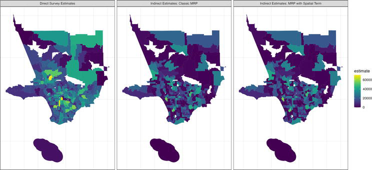
If small area estimates are desired for each geographic area (e.g., each county), the median weighted probability for each poststratification level in each county is then multiplied by the number of known individuals in each county’s matching poststratification level using the poststratification table. These poststratification level-specific outcome estimates are finally grouped by county and summed to create a population-level estimate of the outcome for each county but may be also informative if subpopulation estimates are desired. It is important to note that MRP with a spatial term is not limited to the county level. Figure 2 compares direct estimates of the number of individuals who were vaccinated in the Los Angeles County, California area in September 2020, at the ZIP code (U.S. Census Bureau ZCTA, or ZCTAs) level using traditional survey methods with indirect estimates generated using classic MRP and MRP with a spatial term. While the indirect estimates appear to be virtually identical in this format, and slightly below the direct estimates, when considering aggregated population results in Table 1 it is evident that the spatial term has somewhat improved the estimates, which are closer in total and in variance to the direct estimates. This indicates that using a spatial term for MRP may be an effective way of producing a reliable indirect estimate in the absence of traditional survey weighted direct estimates.

Figure 2.

Comparison of number of vaccinated individuals: Direct survey estimates and indirect estimates (classic MRP and MRP with a spatial term) for ZCTAs in Los Angeles County, California, September 2020.

The direct survey estimates (left) represent the most common approach to generating population estimates of an outcome (in this case, the number of individuals vaccinated in Los Angeles County, California in September 2020 according to survey results from Carnegie Mellon University’s Delphi Group [21]). The direct estimates are slightly higher in certain areas, whereas the indirect estimates appear to be virtually identical in this format. However, when the aggregate estimates are considered (Table 1), it is evident that in this case using MRP with a spatial term subtly improves the estimates. Figure created using ‘ggplot2’ [22] and ‘viridis’ [23] packages in ‘R’.

Method	Estimate (95% confidence interval)	Difference from direct estimate
Direct estimates: survey weights	6807511 (6046260, 7568759)	Baseline
Indirect estimates: classic MRP	6738749 (6119071, 7358432)	18.6% less than baseline
Indirect estimates: MRP with spatial term	6740796 (6118052, 7363537)	18.2% less than baseline

Table 1.

Comparison of direct estimates and MRP estimates: aggregated estimates of the number of vaccinated individuals in ZCTAs approximating Los Angeles County, September 2020.

Table 1 Caption: Direct estimates represent the standard against which to compare the performance of the indirect estimate results. While both indirect estimates from the classic MRP method and the MRP method that uses a spatial term have predicted lower counts of the number of vaccinated individuals in the Los Angeles County, California area in September 2020, it is evident that using MRP with a spatial term has in this instance somewhat improved insofar as the estimate and confidence interval is closer to the direct estimates. While these are small gains, there may be potentially greater gains in analyses where the outcome has even greater spatial dependence.

3.4.2 Spatial data needs and methodological limitations

At this point, it is worth noting that spatial specifications for MRP are only useful if there is spatial structure to the outcome of interest (i.e., the outcome has spatial dependence). Furthermore, it is important to be cautious with the MRP method; whether a spatial term is used, MRP will provide a predicted estimate for every area and every combined demographic category based on the model prediction. It is up to the analyst to determine whether these estimates are reliable or artifacts of predictive modeling using smoothing parameters. Similarly, data availability and richness is important; the spatial model described here requires first-order neighbors, while many missing geographic areas amounting to poor data availability, or else spatial data with little spatial proximity between neighbors (i.e., limited first-order neighbors) will produce unreliable models and potentially incorrect estimates. Consequently, this required data quality and richness is why MRP is often only used in high-income country contexts. If these requirements are ignored, it is possible smoothing parameters may potentially “over-smooth” and create estimates for unobserved areas that are unreliable. Perhaps a reasonable threshold for spatial data missingness is roughly 10%; for example, if we were conducting an analysis of ZCTAs in the whole of the state of California, approximately a maximum of about 10% of the ZCTAs should have missing/unobserved values if we were interested in using spatial specifications, lest the model potentially over-fit the data and produce spurious results.

4. Multilevel regression and poststratification: in application and future developments

Small area estimation procedures have been used to estimate migration patterns (e.g., [24]), homeless population counts (e.g., [25, 26]), and disaster response (e.g., [27]). These applications have had a direct impact on policy and general demographic knowledge. More recently, in collaboration with the World Health Organization [28] Msemburi et al. [29] used SAE methods to understand the impact of COVID-19 in hard to measure parts of the world, including low- and middle-income countries, like India, where health and mortality reporting may not be centralized nor records readily available. They found that between 2020 and 2021, there was a global all-cause excess mortality of 14.9 million people due to the COVID-19 pandemic, with 84% of these deaths in Europe, South-East Asia, and the Americas.

One applied example of MRP using a spatial term for the estimation of difficult-to-measure phenomena is its potential for producing estimates of mortality among under-counted populations, including people experiencing homelessness. In the Seattle, Washington, USA area, deaths among people presumed to have been experiencing homelessness are increasing [30]. While the King County Medical Examiner has collected data pertaining to deaths of individuals presumed to be homeless since 2003, including approximate location of the death and demographic records, these represent only reported and observed deaths. Therefore, the true mortality rate for this vulnerable population is unknown. There may be two ways to estimate the all-cause mortality rate among people experiencing homelessness in Seattle. One way would be to assume the distribution of mortality is similar between the population experiencing homelessness and the total population; people experiencing homelessness are accounted for in the total population mortality. Thus, it would be reasonable to use the records of individual deaths to calculate the percentage of people experiencing homelessness in each demographic stratum in each census tract (i.e., age, sex and race/ethnicity) to fit the model, and use the total population mortality to produce estimates of the percentage of the total population within each demographic stratum in each census tract to poststratify. Another way would be to estimate the percentage of all-cause mortality from the point-in-time (PIT) one-night counts of unhoused people from the Department of Housing and Urban Development [31] to obtain a percentage estimate of mortality for people experiencing homelessness.

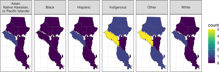
Figure 3 provides a conceptual example of the methods described above. King County Medical Examiner’s Office records for individuals who had died and were presumed to be experiencing homelessness in 2021 [31], as well as Seattle-King County Public Health records for live individuals experiencing homelessness in 2021 [32] were used to produce a binomial logistic regression model of death using only race/ethnicity as a fixed effect, and a BYM2 spatial smoothing term on the city council district (area) in which the individual died or was observed alive. When the city council district was unknown, individuals were randomly assigned to a city council district using population proportions derived from data provided by REACH Evergreen Treatment Services, the largest provider of homelessness stabilization and support services for Seattle-King County Public Health. Poststratification was done based on race/ethnicity in each city council district using data from the United States Department of Housing and Urban Development’s Continuum of Care Point-in-Time counts for Seattle/King County for 2021 [33], and randomly imputing the distribution of each individual by city council district by weighting each area using the proportions from the REACH Evergreen Treatment Services data described above. It was not possible to include both race/ethnicity and age in the MRP process due to a lack of stratum-specific data available. However, it is evident from this figure that there is variation across Seattle city council districts in terms of total mortality as well as race/ethnicity-specific mortality. More demographic strata in the model fitting data, and poststratification data would doubtlessly provide clearer resolution on these trends. Future directions for small area estimation include the use of novel data sources (e.g., geolocated social media posts), extending MRP with spatial terms using in- and out-migration data, and incorporating time components to take advantage of long-term trends among covariates for outcomes of interest.

Figure 3.

Estimated mortality among people experiencing homelessness in Seattle, Washington, USA 2021, poststratified by race/ethnicity and City Council district, using MRP with a spatial term. Indirect estimates of race/ethnicity-specific mortality (counts) among people experiencing homelessness in Seattle, Washington, USA, in 2021 were produced using a binomial logistic regression model of the probability of mortality, with a fixed effect on race/ethnicity category, and a BYM2 spatial smoothing term on city council district (area). Data used for the model included Seattle-King County Public Health records of deaths among individuals presumed to have been experiencing homelessness, as well as data pertaining to observed living persons that included race/ethnicity. Poststratification was achieved using data from the Continuum of Care Point-in-Time counts for Seattle/King County. Figure created using ‘ggplot2’ [22] and ‘viridis’ [23] packages in ‘R’.

5. Conclusion

In this chapter we have reviewed the major importance of small area estimation in demographic and population health fields. Specifically, it is important for demographers and other population scientists to be able to estimate the counts of individuals in arbitrary geographic polygons (e.g., neighborhoods or cities). This is of particular interest for researchers in the Western world interested in non-administrative areas, and those interested in estimating outcomes without high quality census in areas of Africa and parts of Southeast Asia, such as India. Here, we have reviewed the state-of-the-art methods for SAE such as MRP and other statistical smoothing techniques. We have concluded with applications to migration, homelessness and COVID-19.

Acknowledgments

Partial support for this research came from University of Washington Population Health Initiative Grant, a Eunice Kennedy Shriver National Institute of Child Health and Human Development research infrastructure grant, P2C HD042828, and Shanahan Endowment Fellowship, and a Eunice Kennedy Shriver National Institute of Child Health and Human Development training grant, T32 HD101442, to the Center for Studies in Demography & Ecology at the University of Washington. An NSF CAREER Award #2142964 and ARO Award #W911NF-19-1-0407. The content is solely the responsibility of the authors and does not necessarily represent the official views of the NIH, NSF, or ARO.

References

1.Jiang J, Rao JS. Robust small area estimation: An overview. Annual Review of Statistics and Its Application. 2020;7(1):337-360. DOI: 10.1146/annurev-statistics-031219-041212
2.Fay RE, Herriot RA. Estimates of income for small places: An application of James-Stein procedures to Census data. Journal of the American Statistical Association. 1979;74(366):269-277
3.Besag J, York J, Mollié A. Bayesian image restoration with applications in spatial statistics (with discussion). Annals of the Institute of Statistical Mathematics. 1991;43:1-59. DOI: 10.1007/BF00116466
4.Riebler A, Sørbye SH, Simpson D, Rue H. An intuitive Bayesian spatial model for disease mapping that accounts for scaling. Statistical Methods in Medical Research. 2016;25(4):1145-1165. DOI: 10.1177/0962280216660421
5.United States Census Bureau. Small Area Estimation. 2022. Available from: https://www.census.gov/topics/research/stat-research/expertise/small-area-est.html
6.National Cancer Institute. Small Area Estimates for Cancer-Related Measures. 2022. Available from: https://sae.cancer.gov/.
7.United States Census Bureau. Health Insurance. 2022. Available from: https://www.census.gov/topics/health/health-insurance.html
8.Harris V, Caputo J, Finley A, Butler BJ, Bowlick F, Catanzaro P. Small-area estimation for the USDA Forest Service, National Woodland Owner Survey: Creating a fine-scale land cover and ownership layer to support county-level population estimates. Frontiers in Forests and Global Change. 2021;4:1-11. DOI: 10.3389/ffgc.2021.745840
9.Jackman S, Ratcliff S, Mansillo L. Small Area Estimates of Public Opinion: Model-Assisted Post-stratification of Data from Voter Advice Applications [Unpublished Manuscript]. 2019. Available from: https://www.cambridge.org/core/membership/services/aop-file-manager/file/5c2f6ebb7cf9ee1118d11c0a
10.UNICEF. Under-five Mortality. UNICEF DATA; 2023. Available from: https://data.unicef.org/topic/child-survival/under-five-mortality/
11.Gelman A, Little TC. Poststratification into many categories using hierarchical logistic regression. Survey Methodology. 1997;23(2):127-135
12.Gelman A, Lax J, Phillips J, Gabry J, Trangucci R. Using Multilevel Regression and Poststratification to Estimate Dynamic Public Opinion. 2016. p. 2
13.Kastellec JP, Lax JR, Phillips JH. Estimating State Public Opinion With Multi-Level Regression and Poststratification Using R
14.Park DK, Gelman A, Bafumi J. Bayesian multilevel estimation with poststratification: State-level estimates from national polls. Political Analysis. 2004;12(4):375-385
15.Lax JR, Phillips JH. Gay rights in the states: Public opinion and policy responsiveness. American Political Science Review. 2009;103(3):367-386
16.Lax JR, Phillips JH. How should we estimate public opinion in the states? American Journal of Political Science. 2009;53(1):107-121
17.R Core Team. R: A Language and Environment for Statistical Computing. Vienna, Austria: R Foundation for Statistical Computing; 2022. Available from: https://www.R-project.org/
18.Wickham H, Averick M, Bryan J, Chang W, McGowan LD, François R, et al. Welcome to the tidyverse. Journal of Open Source Software. 2019;4(43):1686. DOI: 10.21105/joss.01686
19.Walker K, Herman M. tidycensus: Load US Census Boundary and Attribute Data as ‘tidyverse’ and ‘sf’-Ready Data Frames. R Package Version 1.3.0.9000. 2022. Available from: https://walker-data.com/tidycensus/
20.Rue H, Martino S, Chopin N. Approximate Bayesian inference for latent Gaussian models using integrated nested Laplace approximations (with discussion). Journal of the Royal Statistical Society, Series B. 2009;71(2):319-392. Available from: www.r-inla.org
21.Gao Y, Kennedy L, Simpson D. Treatment effect estimation with multilevel regression and Poststratification. 2021. arXiv preprint arXiv:2102.10003
22.Salomon JA, Reinhart A, Bilinski A, Chua EJ, La Motte-Kerr W, Rönn MM, et al. The US COVID-19 trends and impact survey: Continuous real-time measurement of COVID-19 symptoms, risks, protective behaviors, testing, and vaccination. Proceedings of the National Academy of Sciences. 2021;118(51):e2111454118. DOI: 10.1073/pnas.2111454118
23.Wickham H. ggplot2: Elegant Graphics for Data Analysis. New York: Springer-Verlag; 2016. Available from: https://ggplot2.tidyverse.org
24.Garnier S, Ross N, Rudis R, Camargo PA, Sciaini M, Scherer C. Viridis—Colorblind-friendly color maps for R. 2021 10.5281/zenodo.
25.Hauer M, Byars J. IRS county-to-county migration data, 1990–2010. Demographic Research. 2019;40:1153-1166
26.Almquist ZW, Helwig NE, You Y. Connecting continuum of care point-in-time homeless counts to United States census areal units. Mathematical Population Studies. 2020;27(1):46-58
27.Almquist ZW. Large-scale spatial network models: An application to modeling information diffusion through the homeless population of San Francisco. Environment and Planning B: Urban Analytics and City Science. 2020;47(3):523-540
28.Maas P, Almquist Z, Giraudy E, Schneider JW. Using social media to measure demographic responses to natural disaster: Insights from a large-scale Facebook survey following the 2019 Australia Bushfires. 2020. arXiv preprint arXiv:2008.03665
29.World Health Organization. 14.9 million excess deaths associated with the COVID-19 pandemic in 2020 and 2021 [News release]. 2022. Available from: https://www.who.int/news/item/05-05-2022-14.9-million-excess-deaths-were-associated-with-the-covid-19-pandemic-in-2020-and-2021.
30.Msemburi W, Karlinsky A, Knutson V, Aleshin-Guendel S, Chatterji S, Wakefield J. The WHO estimates of excess mortality associated with the COVID-19 pandemic. Nature (London). 2022;613(7942):130-137. DOI: 10.1038/s41586-022-05522-2
31.King County Medical Examiner’s Office. Homeless Deaths Investigated by the King County Medical Examiner’s Office [Dashboard]. 2022. Available from: https://kingcounty.gov/depts/health/examiner/services/reports-data/homeless.aspx
32.Seattle-King County Public Health. Integrating Data to Better Measure Homelessness. 2023. Available from: https://kingcounty.gov/∼/media/depts/community-human-services/department/documents/KC_DCHS_Cross_Systems_Homelessness_Analysis_Brief_12_16_2021_FINAL.ashx?la=en
33.Department of Housing and Urban Development Exchange. Point-in-Time Count and Housing Inventory Count. 2023. Available from: https://www.hudexchange.info/programs/hdx/pit-hic/
Notes
For the sake of clarity, here “survey data” refers to the unrepresentative data used to build the model, and “census data” are the data representing the known population used to adjust the unrepresentative data and from which population count estimates of the modeled outcome are made. However, it is possible to use large, representative data from the known population such as the American Community Survey 5-year estimates in the United States.
In this case, we have used Integrated Nested Laplace Approximation (INLA), and so more correctly, our example figures are generated using a method that approximates Bayesian processes.
While any geographic level that is present may be used, such as census tract or state, the present discussion will refer to the county level for simplicity.
As determined by the first-order neighborhood structure/grid. First-order neighbor areas share a common geographic boundary, such as immediately neighboring counties.
Typical procedures for building a reasonable model of the outcome of interest may be applied here, including visual interaction checks and model selection processes, but these are beyond the scope of the present discussion.
The present discussion is informed by building a MRP process with spatial specifications using Integrated Nested Laplace Approximation in R (R-INLA) because of INLA’s flexibility in handling spatial models, but similar processes may be undertaken using STAN.
While the mean is often taken for this and subsequent steps in the literature referenced above, perhaps a more Bayesian approach is to take the median.
Written By
Aja M. Sutton and Zack W. Almquist
Submitted: 06 January 2023Reviewed: 15 March 2023Published: 22 June 2023