 Open access peer-reviewed chapter
Abstract
Cancer is one of the most common and deadly diseases worldwide, claiming millions of lives yearly. Despite significant advances in treatment, the overall survival rate remains low, primarily due to late-stage diagnosis. In the high-throughput, high-dimensional omics data era, Biomedical Knowledge should be combined with Data Science best practices for real progress toward precision and personalized medicine. We intuitively and non-technically formulated the main problems or traps and suggested solutions. To illustrate them, we used our Biomedical Data Science platform, i-Biomarker, and its application to circulating miRNA for personalized Multi-Cancer Early Detection and treatment response monitoring, i-Biomarker CaDx. i-Biomarker combines and automates bioinformatics and Explainable AI/ML pipelines. i-Biomarker CaDx works on 32 types of cancer with 99–100% accuracy and is based on more than 30,000 cases.
Keywords
- omics
- Data Science
- Artificial Intelligence
- Multi-Cancer Early Detection
- biomarkers
1. Introduction
Cancer is one of the most common and deadly diseases worldwide, claiming millions of lives yearly. Despite significant advances in treatment, the overall survival rate remains low, primarily due to late-stage diagnosis. Early detection of cancer is critical as it dramatically increases the chance of successful treatment and survival, reducing the overall cost-effectiveness of the treatment (see, e.g., [1, 2]). This underscores the urgent need for more efficient, noninvasive, early cancer detection techniques. Liquid biopsy, a non-invasive procedure that can detect cancer by examining blood samples for cancer-specific markers, has emerged as a promising approach. However, current liquid biopsy tests have several limitations, including modest overall or specific detection rates and robustness (generalizing well to new cases). The main causes, which will be detailed later, are:
The chosen molecular alterations are not informative enough, e.g., circulating DNA methylation for early-stage cancer detection (see [3]).
The size of the inputs is too large relative to the sample size of most clinical studies, which varies between a couple of hundred to a few thousand, for example, more than 1 M nucleosome fragments in cancer early detection [4].
The approach is too simple regarding molecular alterations and/or ML algorithms, for example, combining a cancer type-specific mutation with a known biomarker and modeling with Logistic Regression (see [5]).
Aggressive feature selection often results in models that do not generalize well, for example, trying to reduce the number of biomarkers to just a couple, usually under 10.
Deliberately introducing deviations from Data Science best practice due to some misconceptions, for example, training the model into a cohort and validating it into another one.
In our opinion, in the era of high-throughput, high-dimensional omics data, Biomedical Knowledge should be combined with Data Science best practices for real progress toward
2. Data science issues in biomedical (cancer) test development
2.1 The triad of data science problems
In the realm of Data Science, regardless of the field of application, three primary problems surface universally: classification, regression, and clustering. Each of these problems represents a distinct class of tasks the system needs to solve, their significance extending to a wide array of data-driven fields, including biomedicine.
These three key problems form the foundation for many data science applications in biomedicine, from diagnosing diseases and predicting patient outcomes to stratifying patients for more personalized care. By applying advanced techniques to solve these problems, we can harness the power of data to drive significant advancements in medical science. Using this approach, we built the i-Biomarker™ platform that is agnostic to the disease, omics technology, and biomedical problem and used it to develop the MCED tests (i-Biomarker CaDx).
The natural question is “How can we start with such a general analysis and modeling platform and reach personalized, predictive models that can function as specific tests (e.g., diagnosis or response to treatment prediction) for an individual patient with a particular disease?” The elegant interplay between platform generality and models specificity has the following explanation:
While the platform is general, the data are specific to patients with certain diseases, with their particular measurements and characteristics as inputs.
The clinical outcomes define the particular biomedical problem, for example, diagnosis, prognosis.
Some Explainable AI (XAI) model-agnostic techniques (see e.g., [8]) open the door to personalized prediction explanation.
Armed with highly accurate, personalized biomarkers, Functional Analysis will reveal personalized mechanistic explanations at the molecular level.
Investigating the druggability of altered personalized pathways and molecular networks leads to personalized treatment recommendations.
I-Biomarker has bioinformatic pipelines for the most widely used omics, for example, RNA-seq, Small RNA-seq, Variants (SNP and Indels), Copy Number Variation, Single Cell RNA-seq, CHIP-Seq, Methylation, but here we will focus only on circulating miRNA. The AI/ML i-Biomarker pipelines will be described in another section.
2.1.1 Cancer diagnosis: a classification problem
Cancer diagnosis is essentially a classification problem, where the task is to correctly identify whether a patient has cancer based on a set of input features. This task is often tackled using Artificial Intelligence (AI) and Machine Learning (ML) techniques because they handle complex, high-dimensional data and uncover intricate patterns that traditional statistical methods might miss. A critical aspect of this classification problem, and indeed any data-driven task, is the selection of appropriate input-output pairs. In the realm of biomedicine, and particularly in cancer diagnosis, this selection process can be challenging due to the overwhelming number of potential inputs, or features, that can be measured thanks to advancements in omics technologies. However, it is essential to understand that there must exist a
If the chosen inputs are not informative or relevant to the output, even the most sophisticated AI or ML models, applied with skill, will yield poor accuracy. A common misconception is that simply increasing the number of cases or samples can improve the model’s accuracy. Although a larger sample size can sometimes improve model performance by providing more data to learn from, it cannot compensate for poorly chosen input-output pairs. If the inputs are not informative for the output, adding more samples will not improve the model’s predictive power. For example, the authors of the Grail MCED test, after obtaining an initial detection rate as poor as 16% for stage I and under 50% for stage II cancers, started to perform huge clinical studies, but without any accuracy improvement (see [3]). Therefore, the key to successful AI-driven cancer diagnosis lies in carefully selecting informative and biologically relevant input-output pairs. The right choice can enable AI/ML models to achieve high accuracy, making them valuable tools for early and accurate cancer detection.
2.1.2 Balancing input size and sample size: the curse of dimensionality
One of the key challenges in Data Science, particularly in biomedicine, is the balance between the size of the input data and the number of cases available for analysis. This challenge is commonly called the “curse of dimensionality,” which speaks to the difficulties and complications that arise when dealing with high-dimensional data. In the context of omics data, the input size, or dimensionality, refers to the number of different variables or features that can be measured. For example, about 2500 known miRNAs and 20,000 mRNAs can serve as potential inputs for a model. In contrast, DNA methylation data might include more than 800,000 individual methylation sites, while genomic variant data and fragmentomics [4] can include even more potential inputs. On the other hand, the number of cases, or samples, represents the amount of data available for each of these inputs. In many biomedical research settings, especially those involving rare diseases or specific populations of patients, the number of available samples can be quite limited.
A crucial aspect of model performance is the ratio between the input size and the number of cases. When the number of features (input size) vastly outnumbers the available cases, models can overfit the data, meaning they become too complex and perform well on the training data but poorly on new, unseen data. This issue is further exacerbated when dealing with omics data types with very high input sizes, such as DNA methylation, nucleosome fragmentation, or genomic variants. Here, even with a relatively large number of cases, the sheer number of potential inputs can lead to overfitting, reducing the model’s ability to generalize to new data. Therefore, when working with high-dimensional omics data, it is crucial to carefully balance the input size with the number of available cases. This could involve selecting a subset of the most informative features, using dimensionality reduction techniques, or collecting more data, if possible. By managing this balance effectively, one can mitigate the curse of dimensionality and improve the robustness and generalizability of the model.
However, when the disproportion between the size of the input and the number of cases is huge, for example, nucleosome fragmentation in cancer early detection, having more than 1 M features and a few hundred cases as in Ref. [4], there are serious doubts that using Principal Components Analysis (PCA) for dimensionality reduction solves the problem for several reasons:
Insufficient variability: For PCA to effectively capture the underlying structure of the data, there needs to be sufficient variability across the variables. If you have a small number of cases relative to the high dimensionality of the data, it is likely that the data points will be sparsely distributed in the high-dimensional space. This can result in low variability and make it difficult for PCA to identify meaningful principal components.
Overfitting potential: With a small number of cases, there is a higher risk of overfitting the data when using PCA. Overfitting occurs when the model learns noise or random fluctuations in the data rather than the true underlying patterns. PCA relies on the covariance matrix of the data, and with limited cases, the estimated covariance matrix may not accurately represent the true population covariance structure.
Data standardization challenges: Standardizing the data by subtracting the mean and dividing by the standard deviation is a common preprocessing step in PCA. However, when you have a large number of variables and a small number of cases, calculating reliable means and standard deviations becomes challenging. The estimated mean and standard deviation are more susceptible to being influenced by outliers or extreme values, leading to potentially biased results.
Alternative dimensionality reduction techniques might be more suitable. For example, we could consider methods like sparse PCA, t-SNE (t-distributed Stochastic Neighbor Embedding), or UMAP (Uniform Manifold Approximation and Projection) that are specifically designed to handle these types of data challenges. These methods can offer better results in terms of capturing the underlying structure of the data even with limited cases [9].
2.2 The limitations of traditional biostatistical methods in the age of high-throughput data and AI
Traditional biostatistical methods have provided valuable tools for experimental design and analysis in biomedical research, including formulas to calculate sample size and statistical power. These formulas are designed to ensure that a study is adequately powered, that is, has a sufficient number of cases or samples, to detect a statistically significant effect if one truly exists. However, these traditional methods were developed in a different era of biomedical research, where input size was typically small, the number of available patient data points was limited, and only a handful of statistical algorithms were available to model them. In the era of high-throughput data and AI, the landscape of biomedical research has changed drastically. We now routinely deal with extremely high-dimensional data and have at our disposal a wide range of sophisticated ML algorithms capable of modeling complex relationships. An example of a traditional formula for sample size calculation in a simple comparison of means is as follows:
The sample size (
where:
However, in this formula, there is no explicit consideration for the input size, that is, the dimensionality of the data. This means that the formula might recommend the same sample size, whether your input consists of a few tens of features or hundreds of thousands. The oversimplification here is that traditional formulas assume that each data point is independent of the others, which is often not the case in high-dimensional data, where correlations between features are common. Moreover, they do not account for the “curse of dimensionality” and potential overfitting in the model when the number of features far exceeds the number of cases. In this new era, the traditional biostatistical methods for calculating sample size and power are, therefore, questionable and often inadequate. They fail to capture the complexity and unique challenges of working with high-throughput data and AI models.
As a result, new methods and approaches are required to ensure that we can accurately estimate sample size and power in the context of high-dimensional biomedical data. The so-called learning curves could offer such new solutions, but they need adequate data. There is a large study, TCGA (The Cancer Genome Atlas) [10]), performed on 33 cancer types from over 20,000 primary cancer and matching normal samples using multi-omics techniques (e.g., DNA Methylation, Copy Number Variation, Mutation, miRNA-Seq, and RNA-Seq), which can be used for this purpose.
The above molecular alterations are measured from tissue biopsies (not liquid biopsies), but they can be considered as a proxy, and the data can be used to explore learning curves (unpublished work in progress). As we found that miRNA is the most informative molecular alteration for cancer diagnosis (using TCGA data), of special interest is the evolution of the performance metrics (e.g., accuracy and AUC) versus the sample size and the number of miRNAs. We used this approach in Refs. [11, 12] for TCGA miRNA data and Ensemble of Decision Trees algorithms like Random Forest and XGBoost. We iteratively increase the sample size, run the algorithm, and register the corresponding performance. Moreover, we tried different curve-fitting techniques to find that power laws are the best (see Figures 1 and 2).
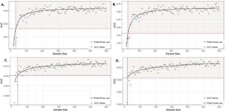
Figure 1.
A and B represent the AUC (area under the curve) and ACC (accuracy) learning curves for random Forest (RF). The corresponding power-low equations, allowing the calculation of the sample size (SS) for a given performance (95% is shown with red dashed lines), are:
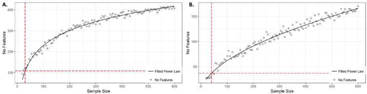
Figure 2.
A. and B. show that the number of features (No features; miRNA here) considered relevant by random Forest (RF) and XGBoost (XGB), respectively, or biomarkers, increase with the sample size (SS), following these formulas:
It is important to note that the learning curves presented do not use hyperparameter tuning. With fine tuning, the highest achievable accuracy is higher, and the number of cases and miRNAs required to reach it is smaller (results not shown).
2.3 The importance of biomarker relationships in predictive models
In the field of biomedicine, biomarkers play a crucial role in the detection, diagnosis, and treatment of diseases. They offer tangible and measurable indicators of physiological or pathological processes or responses to therapeutic intervention. As such, considerable effort is often dedicated to identifying lists of biomarkers associated with specific diseases or conditions. However, in the era of high-throughput data and advanced AI and ML models, the simple identification of a list of biomarkers is no longer sufficient. Rather, the relationship between these biomarkers and the output variable (e.g., disease diagnosis) is of paramount importance. It is perfectly feasible that, given the same list of biomarkers, the best or worst possible predictive model could be developed. This is because the model’s performance does not depend solely on the presence or absence of certain biomarkers. Instead, it is heavily influenced by how these biomarkers interact and relate to the output variable. In essence, it is the intricate patterns and relationships among biomarkers and between biomarkers and the output that provides the predictive power. A performant predictive model does not only consider biomarkers in isolation; it considers their interconnections, their mutual influence, and their collective impact on the output variable. Hence, in the realm of modern biomedicine, we need not only biomarker lists but also performant predictive models that can accurately capture and exploit the complex relationships among these biomarkers. This shift in focus toward model performance and relationship understanding will facilitate more accurate and efficient disease diagnosis, ultimately leading to better patient outcomes.
2.4 Balancing biomarker list size: understanding functional redundancy
One of the ongoing debates in biomedical research revolves around the optimal number of biomarkers for disease detection or prediction. There is a prevalent idea that a minimal set of biomarkers, say less than 10, could offer a cost-effective and highly informative solution. However, this notion often overlooks the complexity of biological systems and their inherent functional redundancy. Evolution has favored designs where information and functionality are distributed among many genes. Even in cases where a few genes act as hubs in complex networks, there are usually other genes involved, contributing to the overall function. This is a concept known as functional redundancy, where the same cellular function can be implemented in multiple alternative ways. Functionally redundant systems provide a buffer against genetic mutations or environmental changes, ensuring the survival and adaptation of organisms.
However, this redundancy presents unique challenges when it comes to biomarker discovery. If multiple interchangeable sets of genes can perform a disease-related function, it implies that no single biomarker or even a small set of biomarkers will be universally indicative of that function. In other words, different patients may have different sets of biomarkers for the same disease due to the functional redundancy of their genetic makeup. Therefore, aggressive feature selection to identify a minimal set of biomarkers could lead to models that perform well on the training set but fail to generalize to new, unseen cases. These models might be overly specific to the particular combinations of biomarkers in the training set and miss other equally valid combinations in the test set.
Consequently, it is essential to strike a balance when determining the size of the biomarker list. While a smaller set of biomarkers might be more practical and cost-effective, a larger set can capture the inherent functional redundancy of biological systems, leading to models that generalize better and are more robust to variability among individual patients.
2.5 Differentially expressed genes: a means to an end, not the end itself
In the domain of omics studies, the identification of differentially expressed genes (DEG) or omics has traditionally been a major focus. DEGs, which show significant differences in expression levels between two or more conditions, can provide valuable insights into the molecular mechanisms underlying these conditions. Thus, many investigators consider the list of DEGs as the end result of a costly omics study.
However, it is critical to understand that identifying DEGs is essentially an Exploratory Data Analysis (EDA) step and not the final goal. The ultimate objective should be to construct robust predictive models that can use these DEGs, among other features, to make accurate predictions about a medical condition such as cancer.
AI and ML methods, especially those with built-in feature selection, are particularly adept at identifying and prioritizing informative features from high-dimensional omics data. In essence, these algorithms are likely to disregard features that are not DEGs, as these features do not show significant differences between the conditions being studied and are thus less likely to be informative. However, the converse is not necessarily true— not all DEGs are equally informative for prediction. AI/ML algorithms typically identify a subset of DEGs that are most relevant for the predictive task at hand. Thus, while DEGs can provide a useful starting point, the final goal should be to develop robust predictive models that effectively utilize these DEGs. In conclusion, although identifying DEGs remains an important step in omics research, it should not be considered the end goal. Instead, the focus should be on using these DEGs to build performant predictive models to inform and improve biomedical decision-making.
3. i-biomarker the Most accurate multi-cancer early detection tests
As we mentioned, i-Biomarker™ is our AI-powered Biomedical Data Science platform [13]. It deals with the entire life cycle of predictive models, illustrated for our MCED test (see Figure 3):
Data Gathering . We collected more than 30,000 cases from freely available international clinical studies that measure circulating miRNA in 32 types of cancer and match normal individuals, using microarray, Next Generation Sequencing (NGS), Polymerase Chain Reaction (PCR), and Nanostring.Data Integration and Cleaning . First, as mentioned above, circulating miRNA profiling can use different technologies and platforms and different miRBase versions. Integrating data from these technologies is beyond the scope of this chapter. Different versions of miRBase have different numbers of miRNAs. In addition to new miRNA discoveries, some miRNAs have disappeared or have been renamed. Thus, we are mapping the miRNA of each study to the last miRBase, which automatically leads to missing values. If an older study is significant regarding the number of cases, its integration limits the number of miRNAs to that known at the corresponding time.Feature Engineering . Besides the usual log2 transformation, we prefer standardization, which transformed the data to mean equal zero and standard deviation equal one. All machine and deep learning algorithms work better with standardized data, which are also easy to interpret—a positive number means increased, while a negative one means decreased. We usually avoid feature selection to better cope with functional redundancy. Also, many of the classification algorithms used in the downstream analysis have built-in feature selection. Additionally, we found that combining features in various ways does not positively impact performance but negatively impacts model interpretability.Model Selection . Usually, we use 12 to 15 classification algorithms (e.g., Random Forest, XGBoost, Support Vector Machines, Deep Learning) on the same training/validation/testing data and compare their performance in terms of either accuracy (the percent of correctly classified cases) or ROC AUC. Figure 4 presents a diagram with the performance of different models, with some, using model amalgamation, reaching performance 1 (100%; maximum) We can select either the best model or the first three or five if we want to combine them.Hyper-parameter Optimization . All classification algorithms have their own parameters. It is possible that with their default values, they do not reach the highest possible accuracy. While i-Biomarker implements many methods, most of the time, random search is a good compromise between the required computational resources and performance.Ensemble . Individual algorithms like Random Forest or Gradient Boosting are already ensembles of decision trees. However, we can pick the best models (even if they are ensembles) and integrate them with different learnable weights in a single model. This is beyond the scope of this chapter but can further increase the accuracy and robustness.Validation . There are some differences in using the validation term in Data Science in general and in biomedical studies. To keep things simple, we will refer shortly only to clinical validation. As we mentioned, one of the problems to be avoided and monitored in Data Science isdata drift . It occurs when the statistics of the new cases are different from the statistics of the data used to build the model. As a result, the accuracy of the model in production alters accordingly. This is a difficult problem, but following the prevailing misconception in the biomedical community, it is deliberately introduced, requiring the model to be trained and validated in different cohorts. Loosely speaking, we want the model to learn as much as possible from the variability existing in the whole population. This can be done by mixing all available cohorts before partitioning the data into train/validation/test sets. Clinical validation is related to regulatory issues to be solved for CE Mark and FDA approval.
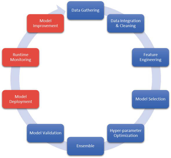
Figure 3.
i-biomarker AI/ML pipeline deals with the entire life cycle of the predictive models as explained in the text.
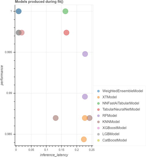
Figure 4.
All models have performance (accuracy) greater than 95%. Some models have performance greater than 99%. Two models detect cancer with 100% accuracy. One of them is a model amalgamation—It integrates other models with different, learnable weights.
The next steps, Model Deployment, Run-time Monitoring, and Model Improvement, are related to production or serving tests like i-Biomarker CaDx to customers (Software as a Service) and will not be addressed in this chapter.
Explainable AI or XAI . Recently, XAI has become increasingly important, especially for clinical decision support systems. We adapted some XAI model-agnostic techniques to enable us to explain the predictions (diagnoses) of both populations (cohort) and individualized models in terms of the corresponding biomarkers.
Population and individual diagnoses are explained as a ranked hierarchy of relevant biomarkers. miRNA biomarkers that support the diagnosis are shown together with those that do not support it and their impact on predictions (see Figure 5).
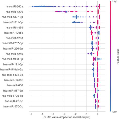
Figure 5.
SHAP values of top features. On the left vertical axis, there is a truncated list of population circulating miRNA discovered by a model amalgamation that detects cancer with 100% precision, ranked by their impact on prediction (relevance). On the right color legend, red/blue indicates a high/low miRNA expression level. On the horizontal axis, we have the SHAP value representing the impact on diagnosis. The sign of the impact indicates the sign or direction of the impact on the cancer diagnosis (not Normal). For example, low values (blue) of hsa-miR-663a have a strong negative impact on cancer diagnosis. Please note that the first four miRNAs have the strongest impact on the cancer diagnosis, while the rest have a decreasing impact. This long-tailed distribution is related to functional redundancy. Each point represents a case; when more than one case has the same SHAP value for the same miRNA, they are stacked vertically.
There is a category of Data Science tools called “What If?” that allows one to alter the values of the relevant features and see how the predictions and the model confidence in them are changing. We modified these tools to monitor the response to treatment, as we realized that any treatment modifies the circulating miRNA values. More precisely, we used a Lung Cancer dataset where, for a subset of cases, we have the circulating miRNA profiles before surgery and after 6 weeks. By giving the new post-operative values of the personalized miRNA biomarkers to the individual predictive model, we can see if the diagnostic and/or its confidence changed (see Figure 6). In fact, by repeating the i-Biomarker CaDx test, we can monitor the patient’s “trajectory” corresponding to all possible evolution under treatment (e.g., progression, recurrence) months before Computed Tomography can detect them.
Population and personalized molecular mechanisms . By using Functional Analysis, we map the population biomarkers discovered onto signaling and metabolic pathways and protein-protein interaction (PPI) to further explain the predictions at the molecular level. We do the same for personalized biomarkers, as they are subsets of the population ones. Thus, personalized molecular mechanisms are revealed. Please note that the accuracy of mechanism identification depends on the precision of personalized predictive models and their corresponding biomarkers. In other words, a low-accuracy predictive model means poor biomarker identification. As these are mapped on the biological networks, it means that mechanisms identification is poor too.Personalized treatment recommendations . By using Network Pharmacology i-Biomarker and its CaDx subsystem can recommend personalized treatment recommendations, based on the druggability of the personalized biological networks alterations.
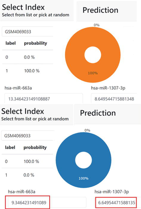
Figure 6.
Personalized response to treatment monitoring. In the upper part, a patient is diagnosed by i-biomarker CaDx with lung cancer, with 100% confidence. An explanation of the diagnosis is given in terms of personalized miRNAs biomarkers values (truncated due to space constraints). In the bottom, the test is repeated 6 weeks after surgery. i-biomarker diagnosed the treated patient as Normal, with 100% confidence and the diagnostic is explained in terms of the new values of the personalized biomarkers (truncated).
4. Conclusions
In the High-throughput and AI Era, developing highly performant diagnoses, prognoses, and responses to treatment prediction tests becomes possible. However, in addition to high-quality informative data, an intuitive understanding of biomedical data science and AI-related problems and their solutions is required. This is enough for the use of platforms like i-Biomarker that combine and automate bioinformatics and AI/ML pipelines. As a proof of concept, we used it to develop the most performant non-invasive multi-cancer early detection and treatment response monitoring test.
Abbreviations
next generation sequencing | |
polymerase chain reaction | |
t-distributed stochastic neighbor embedding | |
uniform manifold approximation and projection | |
the cancer genome atlas | |
exploratory data analysis | |
differential gene expression | |
area under the curve | |
accuracy | |
protein-protein interaction |
References
- 1.
Siegel RL, Miller KD, Fuchs HE, Jemal A. Cancer statistics, 2022. CA: A Cancer Journal for Clinicians. 2022; 72 (1):7-33. [Internet]. Available from:https://onlinelibrary.wiley.com/doi/10.3322/caac.21708 - 2.
GLOBOCAN - Cancer Statistics. 2020. Available from: https://gco.iarc.fr/today/data/factsheets/cancers/39-All-cancers-fact-sheet.pdf - 3.
Pons-Belda OD, Fernandez-Uriarte A, Diamandis EP. Can circulating tumor DNA support a successful screening test for early cancer detection? The grail paradigm. Diagnostics. 2021; 11 (12):2171 [Internet]. Available from:https://www.mdpi.com/2075-4418/11/12/2171 - 4.
Cristiano S, Leal A, Phallen J, Fiksel J, Adleff V, Bruhm DC, et al. Genome-wide cell-free DNA fragmentation in patients with cancer. Nature. 2019; 570 (7761):385-389 [Internet]. Available from:https://www.nature.com/articles/s41586-019-1272-6 - 5.
Cohen JD, Li L, Wang Y, Thoburn C, Afsari B, Danilova L, et al. Detection and localization of surgically resectable cancers with a multi-analyte blood test. Science. 2018; 359 (6378):926-930 [Internet]. Available from:https://www.science.org/doi/10.1126/science.aar3247 - 6.
A novel combination of serum microRNAs for detecting breast cancer in the early stage. Dataset - GSE73002; [Accessed 2023 Mar 2]. Available from: https://www.ncbi.nlm.nih.gov/geo/query/acc.cgi?acc=GSE73002 - 7.
Blood test using serum microRNAs can discriminate lung cancer from non-cancer. Dataset - GSE137140; [Accessed 2023 Mar 2]; 2023. Available from: https://www.ncbi.nlm.nih.gov/geo/query/acc.cgi?acc=GSE137140 - 8.
Christoph M. Interpretable Machine Learning a Guide for Making Black Box Models Explainable. Independently Published (February 28, 2022). Available from: https://christophm.github.io/interpretable-ml-book/ [Accessed: March 2, 2023]. ISBN-13: 979-8411463330 - 9.
Nanga S, Bawah AT, Acquaye BA, Billa MI, Baeta FD, Odai NA, et al. Review of dimension reduction methods. JDAIP. 2021; 09 (03):189-231 [Internet]. Available from:https://www.scirp.org/journal/doi.aspx?doi=10.4236/jdaip.2021.93013 - 10.
The Cancer Genome Atlas Research Network, Weinstein JN, Collisson EA, Mills GB, Shaw KRM, Ozenberger BA, et al. The cancer genome atlas pan-cancer analysis project. Nature Genetics. 2013; 45 (10):1113-1120 [Internet]. Available from:https://www.nature.com/articles/ng.2764 - 11.
Floares A. The smallest sample size for the desired diagnosis accuracy. International Journal of Oncology and Cancer Therapy. 2017; 2 . Available from:https://www.iaras.org/iaras/filedownloads/ijoct/2017/028-0004(2017).pdf . ISSN: 2534-8868 - 12.
Floares AG, Calin GA, Manolache FB. Bigger data is better for molecular diagnosis tests based on decision trees. In: Tan Y, Shi Y, editors. Data Mining and Big Data (Lecture Notes in Computer Science; Vol. 9714). Cham: Springer International Publishing; [Internet]; 2016. pp. 288-295. Available from: http://link.springer.com/10.1007/978-3-319-40973-3_29 - 13.
Artificial Intelligence Expert - Official website describing the platform. 2023. Available from: https://www.aie-op.com/