Mechanical System Kinematics and Dynamics on Differentiable Manifolds

Abstract

Topological and vector space attributes of Euclidean space are employed to create a differentiable manifold structure for holonomic mechanical system kinematics and dynamics. A local kinematic parameterization is presented that establishes the regular configuration space as a differentiable manifold. Topological properties of Euclidean space show that this manifold is naturally partitioned into disjoint, maximal, path connected, singularity free domains of kinematic and dynamic functionality. Using the manifold parameterization, d’Alembert variational equations of mechanical system dynamics yield well-posed ordinary differential equations of motion on these domains, without introducing Lagrange multipliers. Solutions of the differential equations satisfy kinematic configuration, velocity, and acceleration constraints and the variational equations of dynamics. Two examples, one planar and one spatial, are treated using the formulation presented. Solutions obtained are shown to satisfy all three forms of kinematic constraint to within specified error tolerances, using fourth order Runge-Kutta numerical integration methods.

1. Introduction

The objective of establishing a rigorous ordinary differential equation (ODE) formulation for mechanical system dynamics of holonomic systems, without Lagrange multipliers and the associated differential-algebraic equations (DAE) of motion, has been intensively pursued during the past two decades. The motivation for this objective is to avoid the complexity of index 3 DAE of mechanical system dynamics [1]. This paper provides a foundation for a Lagrange multiplier-free ODE formulation of mechanical system dynamics on differentiable manifolds, including existence, uniqueness, and numerical solution on maximal, path connected, domains of singularity free kinematic and dynamic functionality. A benefit of this ODE formulation is rigorous implementation of explicit and implicit ODE numerical integration methods with effective error control for dynamic simulation of a broad spectrum of mechanical systems.

To meet the foregoing objective, a kinematics formulation in Euclidean space is presented in Section 2. Topological and vector space properties of Euclidean space that are needed to establish a differentiable manifold structure for mechanical system kinematics and dynamics are summarized. A triple slider-crank mechanism is used to illustrate topological characteristics of its regular configuration space. A local parameterization of mechanical system kinematics in terms of independent generalized coordinates is presented in Section 3, using vector space properties of Euclidean space and multivariable calculus. It is shown that parameterizations on a system of neighborhoods in the regular configuration space define that space as a differentiable manifold. Practical methods for computation of vector and matrix functions employed in the parameterization are presented. Local properties of the regular configuration space are extended in Section 4 to global form on maximal, path connected, singularity free, disjoint components of the regular configuration manifold. This provides a foundation for reliable simulation and control of mechanical systems on maximal domains of functionality. It is further shown that configurations in disjoint components cannot be connected by continuous singularity free paths in configuration space. Time dependence of the configuration manifold parameterization is defined in Section 5 and used in Section 6 to reduce the d’Alembert variational formulation of mechanical system dynamics to manifold-based ODE of motion, without use of Lagrange multipliers. It is shown that the second order ODE initial-value problem obtained has a unique solution that depends continuously on problem data; i.e., it is well posed on maximal domains of functionality.

The ODE formulation of a five degree of freedom spatial spinning top is presented in Section 7.1, using properties of Euler parameters defined in the Appendix. It is shown that accurate solutions of the ODE are obtained using a fourth order Runge-Kutta integration method and that configuration, velocity, and acceleration constraints are satisfied to near computer precision. The triple slider-crank introduced in Section 2.3 is treated in Section 7.2, where it is shown that dynamic response of the system predicted by the ODE of motion remains in singularity free constraint manifold components. Finally, conclusions are presented in Section 8.

2. Euclidean topological vector spaces and differentiable manifolds

Mechanical systems considered are comprised of rigid bodies whose configurations are defined by $\mathit{ngc}$ generalized coordinates $\mathbf{q}\in {\mathbb{R}}^{\mathit{ngc}}$ that are subject to $\mathit{nhc}$ holonomic constraints (where $\mathit{nhc}<\mathit{ngc}$),

$$\mathtt{\Phi }\left(\mathbf{q}\right)=\mathbf{0}$$E1

It is assumed that the vector function $\mathtt{\Phi }\left(\mathbf{q}\right)={\left[{\mathrm{\Phi }}_1\left(\mathbf{q}\right),\dots ,{\mathrm{\Phi }}_{\mathit{nhc}}\left(\mathbf{q}\right)\right]}^{\mathrm{T}}$ has as many continuous derivatives as needed in the analysis that follows. While the development herein is carried out with constraints that do not depend explicitly on time (scleronomic constraints), the formulation can be extended to time dependent (rheonomic) constraints, with additional terms appearing due to derivatives with respect to time.

2.1 Euclidean topological space

Two related structures are considered on the set

$${\mathbb{R}}^n=\left\{\mathbf{q}={\left[q_1,\dots ,q_n\right]}^{\mathrm{T}},q\in \mathbb{R}\right\}$$

in which kinematics and dynamics of mechanical systems take place. One is the structure of a vector space where addition of elements and multiplication by scalars are defined component-wise, i.e., for $\mathbf{q},{\mathbf{q}}^{\prime }\in {\mathbb{R}}^n$ and $\alpha \in \mathbb{R}$, define

$$\begin{array}{c}\mathbf{q}+{\mathbf{q}}^{\prime }={\left[q_1+q_1^{\prime },\dots ,q_n+q_n^{\prime }\right]}^{\mathrm{T}}\\ \alpha \mathbf{q}={\left[\alpha q_1,\dots ,\alpha q_n\right]}^{\mathrm{T}}\end{array}$$

As a vector space, ${\mathbb{R}}^n$ is $n$-dimensional in the sense that given a linearly independent collection of elements ${\mathbf{q}}^1,\dots ,{\mathbf{q}}^n\in {\mathbb{R}}^n$, every element $\mathbf{q}\in {\mathbb{R}}^n$ can be written uniquely as a linear combination of the form $\mathbf{q}={\alpha }_1{\mathbf{q}}^1+\cdots +{\alpha }_n{\mathbf{q}}^n$. There is also a standard scalar product on ${\mathbb{R}}^n$ given as

$$⟨\mathbf{q},{\mathbf{q}}^{\prime }⟩≔{\mathbf{q}}^{\mathrm{T}}{\mathbf{q}}^{\prime }=\sum _{i=1}^n{q}_i{q}_i^{\prime }.$$

As usual, from a scalar product one can define a norm$\parallel \mathbf{q}\parallel ≔\sqrt{⟨\mathbf{q},\mathbf{q}⟩}$ of a vector $\mathbf{q}$ and the Euclidean distance$d\left(\mathbf{q},{\mathbf{q}}^{\prime }\right)≔\parallel \mathbf{q}-{\mathbf{q}}^{\prime }\parallel$ between vectors $\mathbf{q}$ and ${\mathbf{q}}^{\prime }$.

Although the distance function $d$ is easy to compute and it makes ${\mathbb{R}}^n$ into a metric space, it is not very useful for the study of subspaces of ${\mathbb{R}}^n$. Consider for example two points on a spiral line in a plane; the straight-line Euclidean distance between them completely ignores the geometry of the spiral and is very different from the natural (or intrinsic) distance between the points, which is measured along the spiral. The intrinsic distance is, on the other hand, usually hard to compute as it involves finding geodesic lines between the points. Fortunately, there is a way to avoid these problems by considering the underlying topology on ${\mathbb{R}}^n$ and its subspaces.

Recall that one defines a topology on a set $X$ by declaring some subsets of $X$ to be open. This is done in such a way as to satisfy two simple requirements:

1. an arbitrary union of open sets must be open, and

2. a finite intersection of open sets must be open.

A topological space is thus a set $X$ with a collection of open sets satisfying conditions (1) and (2). A subset $A$ of a topological space naturally inherits the topology by taking as open subsets in $A$ the intersection of $A$ with open subsets of $X$. We will say that $A$ with the inherited topology is a topological subspace of $X$.

It is easy to describe continuous maps between two topological spaces $X$ and $Y$: a function $f:X\to Y$ is continuous if for every open set $U\subseteq Y$ the set $f^{-1}\left(U\right)=\left\{x\in X;f\left(x\right)\in U\right\}$ is an open subset of $X$. Moreover, a bijective map $f:X\to Y$ is called a homeomorphism if both $f$ and its inverse $f^{-1}$ are continuous. Thus, a homeomorphism between topological spaces $X$ and $Y$ determines a bijection between open sets in $X$ and open sets in $Y$.

The topologies of relevance for the purposes of mechanical system kinematics are those that are defined by taking as open sets arbitrary unions of open balls with respect to some distance function $d$. The crucial point here is that different distance functions often generate the same topology. Indeed, in most cases the Euclidean distance and the intrinsic distance on a smooth submanifold $M\subset {\mathbb{R}}^n$ generate the same topology on $M$.

There are two topological properties that are important for kinematics and dynamics of mechanical systems:

1. A topological space is compact if every collection of open sets whose union contains the space can be reduced to a finite sub-collection whose union also contains the entire space. This abstract condition becomes much simpler in Euclidean topological spaces, because a subspace of ${\mathbb{R}}^n$ is compact if it has a finite diameter and if it is closed; i.e., its complement is open in ${\mathbb{R}}^n$.

2. A topological space $X$ is path-connected if for any two points $x.x^{\prime }\in X$ there is a continuous path $\omega :\left[0,1\right]\to X$ starting at $\omega \left(0\right)=x$ and ending at $\omega \left(1\right)=x^{\prime }$. In general, one can define a path-component of a space $X$ as a maximal path-connected subspace of $X$. Every topological space can be decomposed in a unique way as a disjoint union of its path-components.

2.2 Differentiable manifolds

Differentiable manifolds are topological spaces in which one can do differential calculus in a similar manner as in Euclidean spaces. This is achieved by covering a topological space $M$ by open subsets homeomorphic to ${\mathbb{R}}^n$ called ‘charts’, in such a way that whenever two charts overlap there is a transition map between them that is sufficiently differentiable as a map betwen Euclidean spaces.

A more precise definition adapted to our needs is as follows (see [2]): Let $M$ be a topological subspace of some Euclidean topological space ${\mathbb{R}}^n$. A chart on $M$ is an open subset $U\subseteq M$ together with a homeomorphism $\phi$ from $U$ to an open set of ${\mathbb{R}}^m$. A collection of charts $\left\{\left(U_i,{\phi }_i\right)|i=1,2,\dots \right\}$ is a $C^r$-differentiable atlas on $M$ if the charts are compatible in the sense that whenever $U_i\cap U_j\ne \varnothing$, then the transition map

$${\phi }_j\circ {\phi }_i^{-1}:{\phi }_i\left(U_i\cap U_j\right)\to {\phi }_j\left(U_i\cap U_j\right)$$

is at least $r$-times continuously differentiable as a map between $m$-dimensional Euclidean spaces. In order to be able to state and solve second-order ODE, we will require that $r$ is at least 2, but will otherwise simply understand that the transition maps are ‘sufficiently differentiable’. A space $M$ with a differentiable atlas as above is called an $m$-dimensional differentiable manifold (of class $C^r$). Observe that every open subset of $M$ is also a differentiable manifold (of the same dimension and class).

We will frequently use the following construction of differentiable manifolds, based on the Implicit Function Theorem (see [2]). Let $D$ be an open subset of ${\mathbb{R}}^{m+n}$ and let $\mathtt{\Phi }:D\to {\mathbb{R}}^n$ be a differentiable map. A point $\mathbf{q}\in {\mathbb{R}}^{m+n}$ is regular if the Jacobian matrix of $\mathtt{\Phi }$ at $\mathbf{q}$ has rank equal to $n$, and is singular if the rank of that matrix is less than $n$. If $\mathbf{q}$ is a singular point of $\mathtt{\Phi }$, then $\mathtt{\Phi }\left(\mathbf{q}\right)$ is a singular value of $\mathtt{\Phi }$, while the remaining values of $\mathtt{\Phi }$ are regular values. Then we have the following basic fact (see [2], Theorem 1.38): If $\mathbf{v}\in {\mathbb{R}}^n$ is a regular value of $\mathtt{\Phi }$, then

$${\mathtt{\Phi }}^{-1}\left(\mathbf{v}\right)=\left\{\mathbf{q}\in {\mathbb{R}}^{m+n}|\mathtt{\Phi }\left(\mathbf{q}\right)=\mathbf{v}\right\}$$

is an $m$-dimensional differentiable manifold.

2.3 Mechanical system configuration spaces

The configuration space$C$ of a mechanical system is the subset of vectors in ${\mathbb{R}}^{\mathit{ngc}}$ that satisfy Eq. (1),

$$C=\left\{\mathbf{q}\in {\mathbb{R}}^{\mathit{ngc}}|\mathtt{\Phi }\left(\mathbf{q}\right)=\mathbf{0}\right\}$$E2

The configuration space is thus a topological subspace of a Euclidean topological space. Since the constraint equation of Eq. (1) is nonlinear, $\mathtt{\Phi }\left(\mathbf{q}\right)=\mathtt{\Phi }\left({\mathbf{q}}^{\prime }\right)=\mathbf{0}$ does not imply that $\mathtt{\Phi }\left(\mathbf{q}+{\mathbf{q}}^{\prime }\right)=\mathbf{0}$, so $C$ is not in general a vector space. Further, the configuration space may contain configurations at which the $\mathit{nhc}\times \mathit{ngc}$constraint Jacobian matrix,

$${\mathrm{\Phi }}_{\mathbf{q}}\left(\mathbf{q}\right)=\left[\frac{\partial {\mathrm{\Phi }}_i}{\partial q_j}\left(\mathbf{q}\right)\right]$$E3

fails to have full rank. Such configurations are singular, from both kinematic and dynamic points of view [3], and must be avoided.

From a kinematics point of view, if $rank\left({\mathrm{\Phi }}_{\mathbf{q}}\left({\mathbf{q}}^0\right)\right)<\mathit{nhc}$ at some point ${\mathbf{q}}^0\in C$, then in general one cannot find $\mathit{ngc}-\mathit{nhc}$ components of $\mathbf{q}$ that can be used as independent coordinates to represent motion of the system in a neighborhood of ${\mathbf{q}}^0$. In other words, the system does not have $\mathit{ngc}-\mathit{nhc}$degrees of freedom in a neighborhood of ${\mathbf{q}}^0$. From a dynamics point of view, it is not possible to represent dynamics of the system as an ODE in any neighborhood of ${\mathbf{q}}^0$. To avoid these problems, the regular configuration space is defined as

$$\tilde{C}=\left\{\mathbf{q}\in {\mathbb{R}}^{\mathit{ngc}}|\mathrm{\Phi }\left(\mathbf{q}\right)=\mathbf{0}\text{and}rank\left({\mathrm{\Phi }}_{\mathbf{q}}\left(\mathbf{q}\right)\right)=\mathit{nhc}\right\}\subseteq C$$E4

If the set of singular points of $\mathrm{\Phi }$ is a closed subset of $C$, then the regular configuration space is a differentiable manifold of dimension $\mathit{ngc}-\mathit{nhc}$.

2.4 Triple slider-crank mechanism illustration

The planar mechanism shown in Figure 1 is comprised of three sliders that translate along coordinate axes with generalized coordinates $q_1,q_3$ and $q_4$. A crank (body 2) of unit radius is pivoted in and rotates with generalized coordinate $q_2$ relative to slider 1. A distance constraint of unit length acts between the point on the $x_2^{\prime }$-axis shown on the crank periphery and slider 3. Finally, a distance constraint of length 2 units acts between slider 1 and slider 4. Kinematic constraints for this mechanism are

Figure 1.

Triple slider crank mechanism.

$$\mathrm{\Phi }\left(\mathbf{q}\right)=\frac{1}{2}\left[\begin{array}{c}{\left(q_3-q_1-cos{q}_2\right)}^2+{sin}^2{q}_2-1\\ q_1^2+q_4^2-4\end{array}\right]=\frac{1}{2}\left[\begin{array}{c}\left(q_3-q_1\right)\left(q_3-q_1-2cos{q}_2\right)\\ q_1^2+q_4^2-4\end{array}\right]=\mathbf{0}$$E5

and the associated constraint Jacobian is

$${\mathrm{\Phi }}_{\mathbf{q}}\left(\mathbf{q}\right)=\frac{1}{2}\left[\begin{array}{cccc}-\left(q_3-q_1-cos{q}_2\right)& \left(q_3-q_1\right)sin{q}_2& \left(q_3-q_1-cos{q}_2\right)& 0\\ q_1& 0& 0& q_4\end{array}\right]$$E6

Observe that at $q_2=\pm \frac{\pi }{2}$ we have $q_3=q_1$ and the entire first row of the matrix is zero, so the Jacobian fails to have full rank. The solution set $C$ of Eq. (5) is the union of the subsets.

$$C_1=\left\{{\left[q_1{q}_2{q}_1+2cos{q}_2\pm \sqrt{4-q_1^2}\right]}^{\mathrm{T}};-2\le q_1\le 2,0\le q_2\le 2\pi \right\}$$

corresponding to rotations of the crank while sliders 1 and 3 move independently along the axis, and

$$C_2=\left\{{\left[\begin{array}{cccc}{q}_1& q_2& q_1& \pm \sqrt{4-q_1^2}\end{array}\right]}^{\mathrm{T}};-2\le q_1\le 2,0\le q_2\le 2\pi \right\}$$

corresponding to rotations of the crank while the positions of sliders 1 and 3 coincide. Both $C_1$ and $C_2$ are path-connected because one can continuously travel between any two positions within each of the sets. However, $C_1$ and $C_2$ are not path-components of $C$, because

$$C_1\cap C_2=\left\{{\left[\begin{array}{cccc}{q}_1& \pm \pi /2& q_1& \pm \sqrt{4-q_1^2}\end{array}\right]}^{\mathrm{T}};-2\le q_1\le 2,\right\}\ne \varnothing$$

Note that $C_1\cap C_2$ is precisely the set of singular points of the map $\mathrm{\Phi }$. Thus, in our example the configuration space $C$ is two-dimensional and path-connected, but it contains a one-dimensional subset of singular points where $rank\left({\mathrm{\Phi }}_{\mathbf{q}}\left(\mathbf{q}\right)\right)=1<\mathit{nhc}=2$.

By removing singular configurations from $C$ we obtain the regular configuration space $\tilde{C}$ that, as a topological space, splits into four path-components:

$$\begin{array}{l}{\tilde{C}}_1=\left\{{\left[\begin{array}{cccc}{q}_1& q_2& q_1& \pm \sqrt{4-q_1^2}\end{array}\right]}^{\mathrm{T}};-2\le q_1\le 2,-\frac{\pi }{2}\le q_2\le \frac{\pi }{2}\right\}\\ {\tilde{C}}_2=\left\{{\left[\begin{array}{cccc}{q}_1& q_2& q_1& \pm \sqrt{4-q_1^2}\end{array}\right]}^{\mathrm{T}};-2\le q_1\le 2,\frac{\pi }{2}\le q_2\le \frac{3\pi }{2}\right\}\\ {\tilde{C}}_3=\left\{{\left[\begin{array}{cccc}{q}_1& q_2& q_1+2cos{q}_2& \pm \sqrt{4-q_1^2}\end{array}\right]}^{\mathrm{T}};-2\le q_1\le 2,-\frac{\pi }{2}\le q_2\le \frac{\pi }{2}\right\}\\ {\tilde{C}}_4=\left\{{\left[\begin{array}{cccc}{q}_1& q_2& q_1+2cos{q}_2& \pm \sqrt{4-q_1^2}\end{array}\right]}^{\mathrm{T}};-2\le q_1\le 2,\frac{\pi }{2}\le q_2\le \frac{3\pi }{2}\right\}\end{array}$$E7

Within each of these path-components, the Jacobian has maximal rank. Since no rank deficiency of the Jacobian occurs in any of the components of Eq. (7), ODE of motion will be well-posed in each of these path-components (see Section 6). Thus, if the control engineer creates forces and torques that assure the system stays in a path-component, no singularities will be encountered. For example, provided that the torque $\tau$ shown in Figure 1 acting on the crank tends to return the $x_2^{\prime }$ -axis fixed in the crank to coincidence with the $x$-axis and approaches $\infty$ as $q_2$ approached $\pm \pi /2$, dynamic simulation that is initiated in any of the path-components of Eq. (7) will remain in that path-component.

3. Kinematic constraint manifolds

Rather than giving an abstract definition of a kinematic constraint manifold, it is instructive to introduce the concept using properties of the nonlinear equations of kinematics.

3.1 Local parameterization of the regular configuration space

By differentiating Eq. (1) with respect to time we obtain

$${\mathrm{\Phi }}_{\mathbf{q}}\left({\mathbf{q}}^0\right)\dot{\mathbf{q}},$$

so kinematically admissible velocities $\dot{\mathbf{q}}$ at a point ${\mathbf{q}}^0\in \tilde{C}$ are by definition tangent to the regular configuration space at ${\mathbf{q}}^0$.

Let $U$ be the $\mathit{ngc}\times \mathit{nhc}$ matrix ${\mathrm{\Phi }}_{\mathbf{q}}^{\mathrm{T}}\left({\mathbf{q}}^0\right)$, and let $V$ be a $\mathit{ngc}\times \left(\mathit{ngc}-\mathit{nhc}\right)$ matrix whose columns are orthogonal and span the null space of ${\mathrm{\Phi }}_{\mathbf{q}}\left({\mathbf{q}}^0\right)$ ($V$ may be explicitly computed using singular value decomposition [4]). Since by assumption ${\mathrm{\Phi }}_{\mathbf{q}}\left({\mathbf{q}}^0\right)$ has maximal rank, the matrix $U^{\mathrm{T}}U$ is positive definite and we have the relations

$$\begin{array}{l}\mathbf{U}={\mathrm{\Phi }}_{\mathbf{q}}^{\mathrm{T}}\left({\mathbf{q}}^0\right)\\ {\mathbf{U}}^{\mathrm{T}}\mathbf{V}=\mathbf{0}\\ {\mathbf{V}}^{\mathrm{T}}\mathbf{V}=\mathbf{I}\end{array}$$E8

In particular, the columns of $U$ and $V$ span ${\mathbb{R}}^{\mathit{ngc}}$.

We may define a parameterization of $\tilde{C}$ in a neighborhood $U^0\subset \tilde{C}$ of ${\mathbf{q}}^0$ as

$$\mathbf{q}={\mathbf{q}}^0+\mathbf{Vv}-\mathbf{Uu}$$E9

(see Figure 2), which must satisfy

$$\mathrm{\Phi }\left(\mathbf{q}\right)=\mathrm{\Phi }\left({\mathbf{q}}^0+\mathbf{Vv}-\mathbf{Uu}\right)=\mathbf{0}$$E10

We claim that the variables $\mathbf{v}$ and $\mathbf{u}$ comprise a set of local generalized coordinates that are in one-to-one correspondence with $\mathbf{q}$ in $U^0$. To see this, compute $\mathbf{v}$ and $\mathbf{u}$ using Eqs. (9) and (8) as

$$\begin{array}{l}\mathbf{v}={\mathbf{V}}^{\mathrm{T}}\left(\mathbf{q}-{\mathbf{q}}^0\right)\\ \mathbf{u}=-{\left({\mathbf{U}}^{\mathrm{T}}\mathbf{U}\right)}^{-1}{\mathbf{U}}^{\mathrm{T}}\left(\mathbf{q}-{\mathbf{q}}^0\right)\end{array}$$E11

Note that for $\mathbf{q}={\mathbf{q}}^0$ we have ${\mathbf{v}}^0=\mathbf{0}$ and ${\mathbf{u}}^0=\mathbf{0}$.

If we differentiate the function $\mathrm{\Phi }\left({\mathbf{q}}^0+\mathbf{Vv}-\mathbf{Uu}\right)$ with respect to $\mathbf{u}$ we obtain

$$\mathrm{\Phi }{\left({\mathbf{q}}^0+\mathbf{Vv}-\mathbf{Uu}\right)}_{\mathbf{u}}=-{\mathrm{\Phi }}_{\mathbf{q}}\left(\mathbf{q}\right)U$$

In particular, $-{\mathrm{\Phi }}_{\mathbf{q}}\left({\mathbf{q}}^0\right)\mathbf{U}=-{\mathbf{U}}^{\mathrm{T}}\mathbf{U}$ is non-singular, because $U$ has maximal rank. This means that ${\mathbf{u}}^0$ is a regular point of $\mathrm{\Phi }\left({\mathbf{q}}^0+\mathbf{Vv}-\mathbf{Uu}\right)$, viewed as a function of $\mathbf{u}$, so we may apply the Implicit Function Theorem to express $\mathbf{u}$ as a function of $\mathbf{v}$: There exists a neigborhood $V^0\subseteq {\mathbb{R}}^{\mathit{ngc}-\mathit{nhc}}$ of ${\mathbf{v}}^0=\mathbf{0}$ and a unique (sufficiently) differentiable map $\mathbf{h}:V^0\to {\mathbb{R}}^{\mathit{nhc}}$ such that $\mathbf{h}\left({\mathbf{v}}^0\right)={\mathbf{u}}^0$ and

$$\mathbf{u}=\mathbf{h}\left(\mathbf{v}\right)$$

is the locally unique solution of Eq. (10), i.e.,

$$\mathrm{\Phi }\left({\mathbf{q}}^0+\mathbf{Vv}-\mathbf{Uh}\left(\mathbf{v}\right)\right)=\mathbf{0}$$E12

for all $\mathbf{v}\in V^0$. In addition, the formula

$$\mathbf{q}=\mathtt{\Psi }\left(\mathbf{v}\right)≔{\mathbf{q}}^0+\mathbf{Vv}-\mathbf{Uh}\left(\mathbf{v}\right)$$E13

defines a homeomorphism between $V^0$ and a neighborhood $U^0≔\mathrm{\Psi }\left(V^0\right)\subset \tilde{C}$ of ${\mathbf{q}}^0$. In other words, $\left(U^0,{\mathtt{\Psi }}^{-1}\right)$ is a chart on the manifold $\tilde{C}$, as described in Section 2.2. By choosing sufficiently many points ${\mathbf{q}}^0$ we obtain charts that cover the entire regular configuration space $\tilde{C}$. These charts are compatible, because the local parametrizations are defined in the neigbourhood of every point by Eq. (13). Note that the matrix $V$ in Eq. (13) is determined by the Jacobian at a given point, up to an orthogonal change of basis, which does not affect differentiability of transition maps. We thus conclude that $\tilde{C}$ admits a differentiable atlas with local parametrizations given as above. If $\tilde{C}$ is compact, then we can find finitely many charts that cover $\tilde{C}$ and thus work with a finite atlas.

Explicit construction of the parametrization $\mathbf{q}=\mathtt{\Psi }\left(\mathbf{v}\right)$ of the regular configuration space $\tilde{C}$ in a neighborhood $U^0$ of ${\mathbf{q}}^0$ sets the present approach to mechanical system kinematics and dynamics apart from the Maggi/Kane formulation, as presented in [5]. It is also distinct from a substantial literature [6, 7, 8, 9] that derives ODE based on index 1 DAE that do not account for configuration or velocity constraints. The parametrization of Eq. (13) avoids approximation errors at the configuration level.

To see geometrically what Eq. (13) means and why the extent of the neighborhood $V^0$ is important, consider the situation schematically depicted in Figure 2. The vector ${\mathbf{q}}^0+\mathbf{Vv}$ may be viewed as movement in the tangent space of $\tilde{C}$ at ${\mathbf{q}}^0$, which must be modified by vector $-\mathbf{Uu}=-\mathbf{Uh}\left(\mathbf{v}\right)$ to yield $\mathbf{q}\left(\mathbf{v}\right)$ on $\tilde{C}$. Eq. (13) consolidates the vectors into the continuously differentiable function $\mathbf{q}=\mathtt{\Psi }\left(\mathbf{v}\right)$. It is clear from Figure 2, however, that if $\mathbf{v}$ is large, the vector $-\mathbf{Uu}$ that is perpendicular to the tangent space to $\tilde{C}$ at ${\mathbf{q}}^0$ may not intersect $\tilde{C}$, in which case the parametrization fails; i.e., $\mathbf{v}$ is no longer a valid vector of independent generalized coordinates. Fortunately, a large condition number of ${\mathrm{\Phi }}_{\mathbf{q}}\left(\mathbf{q}\right)\mathbf{U}$ [4] is an effective warning that such a situation is eminent, in which case a new vector ${\overline{\mathbf{q}}}^0$ is defined as the current value of $\mathbf{q}$, new bases $\overline{\mathbf{V}}$ and $\overline{\mathbf{U}}$ are evaluated, and analysis is continued with a new mapping $\overline{\mathtt{\Psi }}\left(\overline{\mathbf{v}}\right)$ on neighborhood ${\overline{U}}^0$. The condition number of the kinematic matrix ${\mathrm{\Phi }}_{\mathbf{q}}\left(\mathbf{q}\right)\mathbf{U}$ provides the criterion for definition of charts in the atlas that defines the differentiable manifold $\tilde{C}$. This is a critical link between the kinematics of the system and its differentiable manifold.

Figure 2.

Projection onto $\tilde{C}$.

The mapping of Eq. (13) is a parameterization of open subsets $U^i\subset \tilde{C}$ of the constraint manifold, equivalently the regular kinematic configuration space, by the variable $\mathbf{v}$ on open subsets $V^i\subset {\mathbb{R}}^{\mathit{ngc}-\mathit{nhc}}$. This provides a local mathematical representation of the kinematics of a mechanical system on the linear space ${\mathbb{R}}^{\mathit{ngc}-\mathit{nhc}}$, establishing the fact that the system has $\mathit{ngc}-\mathit{nhc}$ degrees of freedom in $V^0$. The essential nonlinearities of the kinematic system are embedded in the function $\mathtt{\Psi }\left(\mathbf{v}\right)$.

It is important to note that the set $\tilde{C}$ of normalized Euler parameters used to define orientation of a body in space cannot be parameterized by a single mapping from ${\mathbb{R}}^3$ [10]. Thus, constraint manifolds of mechanical systems in space can generally not be parameterized by a single chart. This contradicts some mechanical system dynamics literature that assumes systems can be globally represented using independent generalized coordinates, called Lagrangian coordinates [11].

3.2 Computation of $\mathbf{h}\left(\mathbf{v}\right)$

While the vector function $\mathbf{h}\left(\mathbf{v}\right)$ of Eq. (13) is shown to exist and be a differentiable function of $\mathbf{v}$, the derivation does not show how it may be evaluated. Since it is central to implementing the parameterization defined by Eq. (13), numerical methods for its evaluation are needed. This is pivotal in computational kinematics and dynamics of mechanical systems. If an abstract mathematical approach to manifold theory had been employed, no insight into computation would be obtained. A critical component in iterative computation of $\mathbf{u}=\mathbf{h}\left(\mathbf{v}\right)$ is the matrix ${\mathrm{\Phi }}_{\mathbf{q}}\left(\mathbf{q}\right)\mathbf{U}$ that is nonsingular for $\mathbf{q}\in \tilde{C}$. It defines the matrix

$$\mathbf{B}\left(\mathbf{q}\right)={\left({\mathrm{\Phi }}_{\mathbf{q}}\left(\mathbf{q}\right)\mathbf{U}\right)}^{-1}$$E14

that will play a key role in evaluating $\mathbf{h}\left(\mathbf{v}\right)$ and in obtaining ODE of mechanical system dynamics.

Computation in mechanical system dynamics is carried out on a time grid $t^j$, where $t^0$ is given and $t^j=t^0+\mathit{jh}$, $j=1,2,\dots$, where $h>0$ is a small step size. At $t^0$, ${\mathbf{u}}^0=\mathbf{0}$ and ${\mathbf{B}}^0={\left({\mathbf{U}}^{\mathrm{T}}\mathbf{U}\right)}^{-1}$ is numerically evaluated. At $t^j$, presume ${\mathbf{u}}^j=\mathbf{h}\left({\mathbf{v}}^j\right)$ and ${\mathbf{B}}^j=\mathbf{B}\left({\mathbf{q}}^j\right)$ are known. Equations of motion of Section 6 are formed at $t^j$ and integrated to obtain ${\mathbf{v}}^{j+1}$ and ${\mathbf{q}}^{j+1}$. To solve Eq. (10) for ${\mathbf{u}}^{j+1}=\mathbf{h}\left({\mathbf{v}}^{j+1}\right)$, with a given ${\mathbf{v}}^{j+1}$, set ${\mathbf{u}}_1^{j+1}={\mathbf{u}}^j$, where subscript is iteration number. Newton-Raphson iteration [12] for ${\mathbf{u}}^{j+1}$ is

$${\mathrm{\Phi }}_{\mathbf{u}}^{j+1}\mathrm{\Delta }{\mathbf{u}}_i^{j+1}=-{\mathrm{\Phi }}_{\mathbf{q}}^{j+1}\mathbf{U}\mathrm{\Delta }{\mathbf{u}}_i^{j+1}=-\mathrm{\Phi }\left({\mathbf{q}}^0+{\mathbf{Vv}}^{j+1}-{\mathbf{Uu}}_i^{j+1}\right)$$

Since ${\left({\mathrm{\Phi }}_{\mathbf{q}}^{j+1}\mathbf{U}\right)}^{-1}\approx {\mathbf{B}}^j$ and Newton-Raphson iteration does not require an exact inverse [12], an approximate solution is $\mathrm{\Delta }{\mathbf{u}}_i^{j+1}={\mathbf{B}}^j\mathrm{\Phi }\left({\mathbf{q}}^0+{\mathbf{Vv}}^{j+1}-{\mathbf{Uu}}_i^{j+1}\right)$ and ${\mathbf{u}}_{i+1}^{j+1}={\mathbf{u}}_i^{j+1}+\mathrm{\Delta }{\mathbf{u}}_i^{j+1}$. This yields the iterative algorithm

$${\mathbf{u}}^{i+1}={\mathbf{u}}^i+\mathbf{B}\mathrm{\Phi }\left({\mathbf{q}}^0+\mathbf{Vv}-{\mathbf{Uu}}^i\right),i=1,2,\dots ,\text{until}\parallel \mathrm{\Phi }({\mathbf{q}}^0+{\mathbf{Vv}}^{j+1}-{\mathbf{Uu}}_{i+1}^{j+1}\parallel \le \text{utol}$$E15

where utol is a specified error tolerance. Since the Newton-Raphson method does not require an exact Jacobian, the matrix ${\mathbf{B}}^j$ is held constant throughout the process. This is an efficient computation, requiring only matrix multiplication.

The matrix $\mathbf{B}\left({\mathbf{q}}^{j+1}\right)$ must satisfy Eq. (14), written in the form $\overline{\mathbf{R}}=\left({\mathrm{\Phi }}_{\mathbf{q}}\left(\mathbf{q}\right)\mathbf{U}\right)\mathbf{B}\left(\mathbf{q}\right)-\mathbf{I}=\mathbf{0}$. With an approximation ${\mathbf{B}}_1^{j+1}=\mathbf{B}\left({\mathbf{q}}^j\right)$ of the solution and suppressing the argument $\mathbf{q}$, since it does not change in the iterative process for $\mathbf{B}\left(\mathbf{q}\right)$, the matrix version of Newton-Raphson iteration [3, 12] is defined by $\left({\mathrm{\Phi }}_{\mathbf{q}}^{j+1}\mathbf{U}\right)\mathrm{\Delta }{\mathbf{B}}_i^{j+1}=-{\overline{\mathbf{R}}}_i^{j+1}=-{\mathrm{\Phi }}_{\mathbf{q}}^{j+1}{\mathbf{UB}}_i^{j+1}+\mathbf{I}$. Since the matrix $\left({\mathrm{\Phi }}_{\mathbf{q}}^{j+1}\mathbf{U}\right)$ need not be inverted with great precision for use in the Newton-Raphson process and ${\mathbf{B}}_i^{j+1}\approx {\left({\mathrm{\Phi }}_{\mathbf{q}}^{j+!}\mathbf{U}\right)}^{-1}$, $\mathrm{\Delta }{\mathbf{B}}_i^{j+1}=-{\mathbf{B}}_i^{j+1}{\mathrm{\Phi }}_{\mathbf{q}}^{j+1}{\mathbf{UB}}_i^{j+1}+{\mathbf{B}}_i^{j+1}$ and ${\mathbf{B}}^{i+1}={\mathbf{B}}^i+\mathrm{\Delta }{\mathbf{B}}^i$. This yields the iterative algorithm

$${\mathbf{B}}_{i+1}^{j+1}=2{\mathbf{B}}_i^{j+1}-{\mathbf{B}}_i^{j+1}{\mathrm{\Phi }}_{\mathbf{q}}^{j+1}{\mathbf{UB}}_i^{j+1},i=1,2,\dots ,\text{until}\parallel {\mathrm{\Phi }}_{\mathbf{q}}^{j+1}{\mathbf{UB}}_{i+1}^{j+1}-\mathbf{I}\parallel \le \text{Btol}$$E16

where Btol is a specified error tolerance. This is an efficient computation, requiring only matrix multiplication. If the condition number of the matrix ${\mathrm{\Phi }}_{\mathbf{q}}^{j+1}\mathbf{U}$ exceeds a tolerance that precludes accurate evaluation of its inverse ${\mathbf{B}}^{j+1}$ the numerical process on the time grid is halted, a reparameterization is evaluated, and the process is continued on a new chart.

These results provide practical tools for local parameterization of the regular configuration manifold $\tilde{C}$ and establish a fundamental linkage between topology and the engineering kinematics and dynamics of mechanical systems.

4. Global properties of constraint manifolds in Euclidean space

Results presented in Section 3 are local, in the sense that they are assured to hold only in neighborhoods of configurations involved. For example, a manifold $\tilde{C}$ looks like the Euclidean space ${\mathbb{R}}^{\mathit{nhc}-\mathit{nhc}}$ on a chart $\left(U,\phi \right)$, where $U$ is an open subset of $\tilde{C}$ and $\phi :U\to {\mathbb{R}}^{\mathit{ngc}-\mathit{nhc}}$ is a homeomorphism onto some open subset of ${\mathbb{R}}^{\mathit{ngc}-\mathit{nhc}}$. A metaphor is that a near-sighted person sees the neighborhood $U$ as a Euclidean topological space, even though $\tilde{C}$ in its entirety is not a Euclidean space. This is akin to the early belief that the earth is flat. A powerful impact of differential geometry is that it extends local results to global forms; akin to an optometrist providing corrective lenses to the near-sighted person that sees the earth as flat, showing its nonlinear character by seeing well beyond a neighborhood of one’s feet. Differential geometry is thus a tool, analogous to corrective lenses, that enables observation in the large.

Our local parametrization of $\tilde{C}$ is based on the Implicit Function Theorem, which implies that the intrinsic topology on $\tilde{C}$ given by the differentiable atlas coincides with the topology that $\tilde{C}$ inherits as a subspace of ${\mathbb{R}}^{\mathit{ngc}}$ (see Section 2). In fact, $\tilde{C}$ is a differentiable $\left(\mathit{ngc}-\mathit{nhc}\right)$-dimensional submanifold of ${\mathbb{R}}^{\mathit{ngc}}$. In other words, the number of degrees of freedom is constant (and equal to $\left(\mathit{ngc}-\mathit{nhc}\right)$) throughout the regular configuration spaces. This is not the case on the entire configuration space $C$, which is the principal reason why we restrict our attention to $\tilde{C}$.

In general, $\tilde{C}$ is not a path-connected topological space, even if $C$ itself is path-connected, see for example the Triple Slider-Crank Mechanism in Section 2.4. The path-components of $\tilde{C}$ are maximal, path connected, open subsets of $\tilde{C}$, in each of which the mechanism is locally parameterized by Eq. (13). From a kinematic viewpoint, these path-components are maximal singularity free domains of kinematic functionality, abbreviated domains of functionality.

Extension of the local parameterization of Eq. (13) to a global setting on each ${\tilde{C}}_{\alpha }$ is a powerful result that differential geometry brings to kinematics. While such results are consequences of differential geometry, a deep study of the abstract theory of differential geometry is not required for their use. Once established, implementation of these results requires only use of linear algebra and multivariable calculus.

Given two regular configurations $c_1,c_2$ in the configuration space $C$ several situations may arise. The two configurations may belong to distinct path-components of $C$ so that there does not exist a continuous change of the states of the mechanism that would transform $c_1$ into $c_2$. In general this means that to achieve a transition from the configuration $c_1$ to the configuration $c_2$, the mechanism must be disassembled and then reassembled in some different way. It can also happen that $c_1$ and $c_2$ belong to the same path-component of $C$ but are in different domains of functionality, say ${\tilde{C}}_1$ and ${\tilde{C}}_2$, of the regular configuration space $\tilde{C}$. Different path-components of a manifold are not only disjoint but are what is called topologically separated in the sense that the closure of ${\tilde{C}}_1$ does not intersect ${\tilde{C}}_2$ and vice-versa. This means that every trajectory in the configuration space $C$ along which the mechanism is transformed from $c_1$ to $c_2$ must cross the frontiers of the respective domains of functionality and pass through at least one singularity. In practice this means that in order to pass from $c_1$ to $c_2$, external influence may be exerted at some points to make a continuous transition between different domains of functionality, but the mechanism does not need to be disassemble and reassembled in the process. Nevertheless, it encounters a singularity.

In general, a path between configurations that belong to the same domain of functionality may be constructed as indicated below. If two charts $\left(U_i,{\phi }_i\right)$ and $\left(U_j,{\phi }_j\right)$ defined on $\tilde{C}$ overlap, as shown schematically in Figure 3, then there is a differentiable mapping ${\phi }_j{\phi }_i^{-1}:{\phi }_i\left(U_i\cap U_j\right)\to {\phi }_j\left(U_i\cap U_j\right)$ between intersecting charts and the charts are called compatible, much as two planar maps of the surface of the earth that cover the same locale are compatible. As explained in Section 2.2 a family of compatible charts whose images cover the entire manifold is called an atlas. The atlas provides a structure upon which to characterize trajectories on the constraint manifold, such as a solution curve for the equations of constrained dynamics, as shown schematically in Figure 4. The charts provide for changes in local coordinates along a trajectory $\mathbf{q}\left(\mathbf{v}\left(t\right)\right)$ in ${\tilde{C}}_{\alpha }$, including differentiability of generalized coordinates and tangents. The theory of differentiable manifolds [2] assures that a solution trajectory can be continued in the open submanifold $\tilde{C}$ until the constraint Jacobian ${\mathrm{\Phi }}_{\mathbf{q}}\left(\mathbf{q}\right)$ becomes rank deficient. While the theory does not explicitly determine the extent of components of the regular configuration manifold, it does assure that the parameterization by charts that has been presented is valid on the largest possible subset of regular configuration space. Nothing more is possible.

Figure 3.

Continuation of solution trajectory over charts.

Figure 4.

Symmetric top with tip constrained to be unit distance from origin O.

5. Kinematics as a function of time

In Section 3 we obtained an explicit expression (Eq. 13) for configurations $\mathbf{q}\in \tilde{C}$ in terms of local coordinates $\mathbf{v}\in {\mathbb{R}}^{\mathit{ngc}-\mathit{nhc}}$. In this section we continue this work and give explicit expressions for $\dot{\mathbf{q}}$ and $\ddot{\mathbf{q}}$ in terms of $\mathbf{v},\dot{\mathbf{v}}$ and $\ddot{\mathbf{v}}$. For dynamics of mechanical systems, generalized coordinates are a function of time, $\mathbf{q}=\mathbf{q}\left(t\right)$. By differentiating Eq. (1) with respect to time we obtain a velocity constraint equation

$${\mathrm{\Phi }}_{\mathbf{q}}\left(\mathbf{q}\right)\dot{\mathbf{q}}=\mathbf{0}$$E17

Furthermore, a second derivative with respect to time yields $\dot{(}{\mathrm{\Phi }}_{\mathbf{q}}\left(\mathbf{q}\right))\dot{\mathbf{q}}+{\mathrm{\Phi }}_{\mathbf{q}}\left(\mathbf{q}\right)\ddot{\mathbf{q}}=\mathbf{0}$ (where $\dot{(}{\mathrm{\Phi }}_{\mathbf{q}}\left(\mathbf{q}\right))$ denotes the component-wise derivative of the Jacobian matrix ${\mathrm{\Phi }}_{\mathbf{q}}\left(\mathbf{q}\right)$ with respect to $t$). Thus we obtain an acceleration constraint equation

$${\mathrm{\Phi }}_{\mathbf{q}}\left(\mathbf{q}\right)\ddot{\mathbf{q}}=-\dot{(}{\mathrm{\Phi }}_{\mathbf{q}}\left(\mathbf{q}\right))\dot{\mathbf{q}}=-\gamma \left(\mathbf{q},\dot{\mathbf{q}}\right),$$E18

where we abbreviated

$$\gamma \left(\mathbf{q},\dot{\mathbf{q}}\right)≔\dot{(}{\mathrm{\Phi }}_{\mathbf{q}}\left(\mathbf{q}\right))\dot{\mathbf{q}}$$E19

Eqs. (1), (17) and (18) represent three forms of constraint that must be satisfied by $\mathbf{q}\in \tilde{C}$.

With time held fixed, Eq. (17) yields

$${\mathrm{\Phi }}_{\mathbf{q}}\left(\mathbf{q}\right)\delta \mathbf{q}=\mathbf{0}$$E20

which defines kinematically admissible virtual displacements$\delta \mathbf{q}$ [3, 11] that are tangent to the regular configuration space.

Let us begin with two auxiliary results that will be used in computation. By differentiating Eq. (13) with respect to $t$, we get

$$\dot{\mathbf{q}}=\mathbf{V}\dot{\mathbf{v}}-\mathbf{U}\dot{\mathbf{h}},$$E21

which together with Eq. (17) yields

$${\mathrm{\Phi }}_{\mathbf{q}}\left(\mathbf{q}\right)\mathbf{V}\dot{\mathbf{v}}={\mathrm{\Phi }}_{\mathbf{q}}\left(\mathbf{q}\right)\mathbf{U}\dot{\mathbf{h}}$$E22

Furthermore, in Section 3 we observed that ${\mathrm{\Phi }}_{\mathbf{q}}\left(\mathbf{q}\right)U$ is invertible in a neighborhood of ${\mathbf{q}}^0$, so we may define the matrix inverse

$$\mathbf{B}\left(\mathbf{q}\right)≔{\left({\mathrm{\Phi }}_{\mathbf{q}}\left(\mathbf{q}\right)U\right)}^{-1}.$$

of Eq. (14). By differentiating the equality $\mathbf{B}{\mathrm{\Phi }}_{\mathbf{q}}U=\mathbf{I}$ with respect to $t$ we obtain $\dot{\mathbf{B}}{\mathrm{\Phi }}_{\mathbf{q}}U+\mathbf{B}{\dot{\mathrm{\Phi }}}_{\mathbf{q}}U=\mathbf{0}$, therefore

$$\dot{\mathbf{B}}{\mathrm{\Phi }}_{\mathbf{q}}U=-\mathbf{B}{\dot{\mathrm{\Phi }}}_{\mathbf{q}}U$$E23

It is now easy to compute $\dot{\mathbf{q}}$ (we suppress arguments):

$$\begin{array}{l}\dot{\mathbf{q}}=\mathbf{V}\dot{\mathbf{v}}-\mathbf{U}\dot{\mathbf{h}}\mathrm{by}\mathrm{Eq}.\left(21\right)\\ =\mathbf{V}\dot{\mathbf{v}}-\mathbf{UB}{\mathrm{\Phi }}_{\mathbf{q}}\mathbf{U}\dot{\mathbf{h}}\text{using}\mathbf{B}{\mathrm{\Phi }}_{\mathbf{q}}\mathbf{U}=\mathbf{I}\\ =\mathbf{V}\dot{\mathbf{v}}-\mathbf{UB}{\mathrm{\Phi }}_{\mathbf{q}}\mathbf{V}\dot{\mathbf{v}}\mathrm{by}\mathrm{Eq}.\left(22\right)\\ =\mathbf{D}\dot{\mathbf{v}}\text{we\hspace{0.17em}abbreviate}\mathbf{D}\left(\mathbf{q}\right)≔\left(\mathbf{I}-\mathbf{UB}\left(\mathbf{q}\right){\mathrm{\Phi }}_{\mathbf{q}}\left(\mathbf{q}\right)\right)\mathbf{V}\end{array}$$E24

Observe that the matrix function $\mathbf{D}\left(\mathbf{q}\right)$ satisfies

$${\mathrm{\Phi }}_{\mathbf{q}}\mathbf{D}=\left({\mathrm{\Phi }}_{\mathbf{q}}-{\mathrm{\Phi }}_{\mathbf{q}}\mathbf{UB}{\mathrm{\Phi }}_{\mathbf{q}}\right)\mathbf{V}=\left({\mathrm{\Phi }}_q-{\mathrm{\Phi }}_{\mathbf{q}}\right)\mathbf{V}=\mathbf{0},$$E25

which means that the columns of $\mathbf{D}\left(\mathbf{q}\right)$ comprise a continuously differentiable basis for the null space of ${\mathrm{\Phi }}_{\mathbf{q}}$.

In order to express $\ddot{\mathbf{q}}$, we differentiate Eq. (24) with respect to $t$:

$$\ddot{\mathbf{q}}=\mathbf{D}\ddot{\mathbf{v}}+\dot{\mathbf{D}}\dot{\mathbf{v}}$$E26

and compute

$$\begin{array}{ll}\dot{\mathbf{D}}\dot{\mathbf{v}}=-\left(\mathbf{U}\dot{\mathbf{B}}{\mathrm{\Phi }}_{\mathbf{q}}\mathbf{V}+\mathbf{UB}{\dot{\mathrm{\Phi }}}_{\mathbf{q}}\mathbf{V}\right)\dot{\mathbf{v}}& \\ =-\mathbf{U}\dot{\mathbf{B}}{\mathrm{\Phi }}_{\mathbf{q}}\mathbf{U}\dot{\mathbf{h}}-\mathbf{UB}{\dot{\mathrm{\Phi }}}_{\mathbf{q}}\mathbf{V}\dot{\mathbf{v}}& \mathrm{by}\mathrm{Eq}.\left(22\right)\\ =\mathbf{UB}{\dot{\mathrm{\Phi }}}_{\mathbf{q}}\mathbf{U}\dot{\mathbf{h}}-\mathbf{UB}{\dot{\mathrm{\Phi }}}_{\mathbf{q}}\mathbf{V}\dot{\mathbf{v}}& \mathrm{by}\mathrm{Eq}.\left(23\right)\\ =\mathbf{UB}{\dot{\mathrm{\Phi }}}_{\mathbf{q}}\left(\mathbf{U}\dot{\mathbf{h}}-\mathbf{V}\dot{\mathbf{v}}\right)=-\mathbf{UB}\gamma & \mathrm{by}\mathrm{Eq}.\left(19\right)\end{array}$$E27

By combining Eqs. (26) and (27) we obtain

$$\ddot{\mathbf{q}}=\mathbf{D}\left(\mathbf{q}\right)\ddot{\mathbf{v}}-\mathbf{UB}\left(\mathbf{q}\right)\gamma \left(\mathbf{q},\dot{\mathbf{q}}\right)$$E28

We may finally summarize Eqs. (13), (24) and (28) that define $\mathbf{q},\dot{\mathbf{q}},\ddot{\mathbf{q}}$ as functions of $\mathbf{v},\dot{\mathbf{v}},\ddot{\mathbf{v}}$.‘

$$\begin{array}{l}\mathbf{q}\left(\mathbf{v}\right)={\mathbf{q}}^0+\mathbf{Vv}-\mathbf{Uh}\left(\mathbf{v}\right)\\ \dot{\mathbf{q}}\left(\mathbf{v},\dot{\mathbf{v}}\right)=\mathbf{D}\left(\mathbf{q}\left(\mathbf{v}\right)\right)\dot{\mathbf{v}}\\ \ddot{\mathbf{q}}\left(\mathbf{v},\dot{\mathbf{v}},\ddot{\mathbf{v}}\right)=\mathbf{D}\left(\mathbf{q}\left(\mathbf{v}\right)\right)\ddot{\mathbf{v}}-\mathbf{UB}\left(\mathbf{q}\left(\mathbf{v}\right)\right)\gamma \left(\mathbf{q}\left(\mathbf{v}\right),\dot{\mathbf{q}}\left(\mathbf{v},\dot{\mathbf{v}}\right)\right)\end{array}$$E29

We have thus demonstrated that $\mathbf{q}$, $\dot{\mathbf{q}}$ and $\ddot{\mathbf{q}}$ are differentiable functions of $\mathbf{v}$, $\dot{\mathbf{v}}$ and $\ddot{\mathbf{v}}$ and provided explicit formulae to describe $\mathbf{q}$, $\dot{\mathbf{q}}$ and $\ddot{\mathbf{q}}$ that satisfy constraint Eqs. (1), (17) and (18), once independent coordinates $\mathbf{v}$, $\dot{\mathbf{v}}$ and $\ddot{\mathbf{v}}$ are determined as a solution of equations of dynamics presented in Section 6.

The importance of the fact that generalized coordinates $\mathbf{q}$ and their derivatives $\dot{\mathbf{q}}$ and $\ddot{\mathbf{q}}$ identically satisfy the holonomic, velocity and acceleration constraints in a neighborhood of ${\mathbf{q}}^0$ cannot be overemphasized. This aspect of the differentiable manifold formulation is critical in avoiding so called constraint drift that is associated with many mechanical system dynamics formulations that are based on approximations and their numerical implementations with projections onto the constraint manifold, see [6, 7, 8, 9, 13, 14].

6. Manifold-based ODE of mechanical system dynamics

Using the foregoing manifold-based kinematics formulation, the variational equation of motion for a holonomic system is reduced to a system of ODE. The d’Alembert variational equation of motion for a mechanical system is [3, 11].

$$\delta {\mathbf{q}}^{\mathrm{T}}\left(\mathbf{Mq}\ddot{\mathbf{q}}-\mathbf{S}\left(\mathbf{q},\dot{\mathbf{q}}\right)-{\mathbf{Q}}^A\left(\mathbf{q},\dot{\mathbf{q}},t\right)\right)=0$$E30

which must hold for all $\delta \mathbf{q}$ that satisfy Eq. (20); i.e., ${\mathrm{\Phi }}_{\mathbf{q}}\delta \mathbf{q}=\mathbf{0}$, for a system with holonomic constraints of Eq. (1) that include Euler parameter normalization conditions for spatial bodies. Terms appearing in Eq. (30) are the mass matrix $\mathbf{M}\left(\mathbf{q}\right)$ that is symmetric and positive definite on the null space of ${\mathrm{\Phi }}_{\mathbf{q}}\left(\mathbf{q}\right)$ [3], velocity coupling terms $\mathbf{S}\left(\mathbf{q},\dot{\mathbf{q}}\right)$ that are quadratic in $\dot{\mathbf{q}}$, and generalized applied force ${\mathbf{Q}}^A\left(\mathbf{q},\dot{\mathbf{q}},t\right)$. It should be noted that for spatial systems with orientation defined by Euler parameters, $\mathbf{M}\left(\mathbf{q}\right)$ is singular. Nevertheless, it is positive definite on the null space of ${\mathrm{\Phi }}_{\mathbf{q}}\left(\mathbf{q}\right)$.

As in Eq. (24), with time held fixed, $\delta \mathbf{q}=\mathbf{D}\left(\mathbf{q}\right)\delta \mathbf{v}$. Using this relation and Eq. (29), Eq. (30) reduces to a variational equation in $\mathbf{v}$,

$$\delta {\mathbf{v}}^{\mathrm{T}}{\mathbf{D}}^{\mathrm{T}}\left(\mathbf{q},t\right)\left(\mathbf{M}\left(\mathbf{q}\right)\mathbf{D}\left(\mathbf{q}\right)\ddot{\mathbf{v}}-\mathbf{M}\left(\mathbf{q}\right)\mathbf{UB}\left(\mathbf{q}\right)\gamma \left(\mathbf{q},\dot{\mathbf{q}}\right)-\mathbf{S}\left(\mathbf{q},\dot{\mathbf{q}}\right)-{\mathbf{Q}}^A\left(\mathbf{q},\dot{\mathbf{q}},t\right)\right)=0$$E31

From Eq. (25),

$${\mathrm{\Phi }}_{\mathbf{q}}\left(\mathbf{q}\right)\delta \mathbf{q}={\mathrm{\Phi }}_{\mathbf{q}}\left(\mathbf{q}\right)\mathbf{D}\left(\mathbf{q}\right)\delta \mathbf{v}=\mathbf{0}$$

for arbitrary $\delta \mathbf{v}$. Thus, Eq. (31) holds for arbitrary $\delta \mathbf{v}$ and, suppressing arguments,

$${\mathbf{D}}^{\mathrm{T}}\mathbf{MD}\ddot{\mathbf{v}}={\mathbf{D}}^{\mathrm{T}}\left(\mathbf{MUB}\gamma +\mathbf{S}+{\mathbf{Q}}^A\right)$$E32

where Eq. (29) shows that $\mathbf{q}$ and $\dot{\mathbf{q}}$ are functions of $\mathbf{v}$ and $\dot{\mathbf{v}}$, and

$$\begin{array}{l}\mathbf{M}\left(\mathbf{q}\left(\mathbf{v}\right)\right)=\mathbf{M}\left(\mathbf{v}\right)\\ \gamma \left(\mathbf{q}\left(\mathbf{v}\right),\dot{\mathbf{q}}\left(\mathbf{v},\dot{\mathbf{v}}\right)\right)=\gamma \left(\mathbf{v},\dot{\mathbf{v}}\right)\\ \mathbf{S}\left(\mathbf{q}\left(\mathbf{v}\right),\dot{\mathbf{q}}\left(\mathbf{v},\dot{\mathbf{v}}\right)\right)=\mathbf{S}\left(\mathbf{v},\dot{\mathbf{v}}\right)\\ {\mathbf{Q}}^A\left(\mathbf{q}\left(\mathbf{v}\right),\dot{\mathbf{q}}\left(\mathbf{v},\dot{\mathbf{v}}\right),t\right)={\mathbf{Q}}^A\left(\mathbf{v},\dot{\mathbf{v}},t\right)\\ \mathbf{B}\left(\mathbf{q}\left(\mathbf{v}\right)\right)=\mathbf{B}\left(\mathbf{v}\right)\\ \mathbf{D}\left(\mathbf{q}\left(\mathbf{v}\right)\right)=\mathbf{D}\left(\mathbf{v}\right)\end{array}$$E33

Eq. (32) is thus a second order ODE in $\mathbf{v}$.

At an initial configuration ${\mathbf{q}}^0$ that satisfies Eq. (1), ${\mathrm{\Phi }}_{\mathbf{q}}\left({\mathbf{q}}^0\right)\mathbf{V}=\mathbf{0}$ and ${\mathbf{D}}^0=\mathbf{D}\left({\mathbf{q}}^0\right)=\mathbf{V}-\mathbf{UB}\left({\mathbf{q}}^0\right){\mathrm{\Phi }}_{\mathbf{q}}\left({\mathbf{q}}^0\right)\mathbf{V}=\mathbf{V}$. Thus, ${\mathbf{D}}^{0T}\mathbf{M}\left({\mathbf{q}}^0\right){\mathbf{D}}^0={\mathbf{V}}^{\mathrm{T}}\mathbf{M}\left({\mathbf{q}}^0\right)\mathbf{V}$. Since the columns of $\mathbf{V}$ form a basis for the null-space of ${\mathrm{\Phi }}_{\mathbf{q}}\left({\mathbf{q}}^0\right)$, on which $\mathbf{M}\left({\mathbf{q}}^0\right)$ is positive definite, the symmetric reduced mass matrix ${\mathbf{D}}^{\mathrm{T}}\left(\mathbf{v}\right)\mathbf{M}\left(\mathbf{v}\right)\mathbf{D}\left(\mathbf{v}\right)$ of Eq. (32), which is a continuous function of $\mathbf{v}$, is positive definite, hence nonsingular, in a neighborhood of ${\mathbf{v}}^0=\mathbf{0}$. Multiplying both sides of Eq. (32) by the inverse of ${\mathbf{D}}^{\mathrm{T}}\mathbf{MD}$, suppressing arguments of functions involved for notational simplicity, yields the traditional form of a second order ODE,

$$\ddot{\mathbf{v}}={\left({\mathbf{D}}^{\mathrm{T}}\mathbf{MD}\right)}^{-1}{\mathbf{D}}^{\mathrm{T}}\left(\mathbf{MUB}\gamma +\mathbf{S}+{\mathbf{Q}}^A\right)≔\mathbf{g}\left(\mathbf{v},\dot{\mathbf{v}},t\right)$$E34

Given initial values of $\mathbf{q}\left(t^0\right)$ and $\dot{\mathbf{q}}\left(t^0\right)$ that satisfy Eqs. (1) and (17) at $t^0$ we obtain initial conditions on $\mathbf{v}$ and $\dot{\mathbf{v}}$,

$$\begin{array}{l}\mathbf{v}\left(t^0\right)=\mathbf{0}\\ \dot{\mathbf{v}}\left(t^0\right)={\mathbf{V}}^{\mathrm{T}}\dot{\mathbf{q}}\left(t^0\right)\end{array}$$E35

Assuming all functions that appear in Eq. (33) are continuously differentiable with respect to their arguments, the initial-value problem of Eqs. (34) and (35) has a unique solution for $\mathbf{v}\left(t\right)$ in a neighborhood of $\left({\mathbf{v}}^0,t^0\right)$ [15]. As shown in Section 4.1, this solution can be continued on the constraint manifold shown schematically in Figure 3 until a singular configuration or the desired final time $t^f$ is encountered. Further, if terms in Eq. (33) are $k$-times continuously differentiable with respect to a vector $\mathbf{b}$ of parameters, so is the solution [15]. With these existence, uniqueness, and differentiability properties, the initial-value problem of Eqs. (34) and (35) is well posed.

Numerical reduction of variational equations of motion to ODE depends on tolerances utol in approximating $\mathbf{u}$ and Btol in approximating $\mathbf{B}$ in Eqs. (15) and (16). Thus, after numerical solution of the ODE of motion for $\mathbf{v}$ and its derivatives, Eq. (29) yields $\mathbf{q},\dot{\mathbf{q}},\ddot{\mathbf{q}}$ that satisfy the constraints of Eqs. (1), (17), and (18), to within specified error tolerances. More specifically, the accuracy with which the configuration generalized coordinates $\mathbf{q}$ are evaluated depends on the accuracy with which $\mathbf{u}$ is computed in Eq. (15); i.e., utol. As long as convergence in this iteration is achieved, the accuracy with which $\mathbf{B}$ is computed in Eq. (15) is immaterial. In contrast, the accuracy of $\dot{\mathbf{q}}$ and $\ddot{\mathbf{q}}$ that are computed in Eq. (29) is directly impacted by the accuracy with which $\mathbf{B}$ is computed in Eq. (16); i.e., Btol. Thus, both utol and Btol control the accuracy with which velocity and acceleration generalized coordinates are evaluated.

It is noted that with the unique solution of Eqs. (34) and (35) and its derivatives known, Eq. (29) determines the unique solution $\mathbf{q}\left(t\right)$ and its derivatives of the mechanical system dynamics problem. As emphasized earlier, this solution satisfies all three forms of holonomic constraint, to within specified tolerances. Thus, problems associated with drift from constraints that arise in numerical treatments of the DAE of mechanical system dynamics that fail to enforce all forms of constraint are not of concern. Similarly, errors induced by use of an approximate ODE and modification of results to satisfy constraints are avoided.

7. Numerical examples

Two examples are treated using the manifold-based ODE formulation. The first is a five degree of freedom spatial spinning Top whose tip is constrained to be a unit distance from a point fixed in space. The second example is the planar triple slider-crank of Section 2.4. Its dynamics in two of the four disjoint singularity free domains of functionality defined in Eq. (7) are simulated using an extended four body planar model with generalized coordinates in ${\mathbb{R}}^{\mathit{ngc}}={\mathbb{R}}^{12}$, while retaining its two degrees of freedom.

7.1 Symmetric top with tip constrained to be a unit distance from a fixed point

Consider a symmetric Top with its tip that is 1 m from the centroid constrained to be 1 m from the origin of the $x-y-z$ frame, as shown in Figure 4. In this model, $\mathbf{q}={\left[{\mathbf{r}}^{\mathrm{T}}{\mathbf{p}}^{\mathrm{T}}\right]}^{\mathrm{T}}$, where $\mathbf{p}\in {\mathbb{R}}^4$ is the vector of Euler parameters defined in the Appendix that characterizes orientation of the body fixed $x^{\prime }-y^{\prime }-z^{\prime }$ reference frame. In addition to the Euler parameter normalization constraint of Eq. (37) in the Appendix, the length of vector $\mathbf{s}=\mathbf{r}-\mathbf{A}\left(\mathbf{p}\right){\mathbf{u}}_{z^{\prime }}$ shown in Figure 4 must be unity, i.e.,

$${\mathbf{s}}^{\mathrm{T}}\mathbf{s}={\left(\mathbf{r}-\mathbf{A}\left(\mathbf{p}\right){\mathbf{u}}_{z^{\prime }}\right)}^{\mathrm{T}}\left(\mathbf{r}-\mathbf{A}\left(\mathbf{p}\right){\mathbf{u}}_{z^{\prime }}\right)={\mathbf{r}}^{\mathrm{T}}\mathbf{r}-2{\mathbf{r}}^{\mathrm{T}}\mathbf{A}\left(\mathbf{p}\right){\mathbf{u}}_{z^{\prime }}+1=1$$

Holonomic constraints for the system are thus

$$\mathrm{\Phi }\left(\mathbf{q}\right)=\frac{1}{2}\left[\begin{array}{c}{\mathbf{r}}^{\mathrm{T}}\mathbf{r}-2{\mathbf{r}}^{\mathrm{T}}\mathbf{A}\left(\mathbf{p}\right){\mathbf{u}}_{z^{\prime }}\\ {\mathbf{p}}^{\mathrm{T}}\mathbf{p}-1\end{array}\right]=\mathbf{0}$$

Using Eq. (39) of the Appendix, the constraint Jacobian is

$${\mathrm{\Phi }}_{\mathbf{q}}\left(\mathbf{q}\right)=\left[\begin{array}{cc}{\mathbf{r}}^{\mathrm{T}}-{\mathbf{u}}_{z^{\prime }}^{\mathrm{T}}{\mathbf{A}}^{\mathrm{T}}\left(\mathbf{p}\right)& -{\mathbf{r}}^{\mathrm{T}}\mathbf{B}\left(\mathbf{p},{\mathbf{u}}_{z^{\prime }}\right)\\ \mathbf{0}& {\mathbf{p}}^{\mathrm{T}}\end{array}\right]$$

To determine if the Jacobian has full rank, form the equation

$${\mathrm{\Phi }}_{\mathbf{q}}{\left(\mathbf{q}\right)}^{\mathrm{T}}\left[\begin{array}{c}\alpha \\ \beta \end{array}\right]=\left[\begin{array}{c}\left(\mathbf{r}-\mathbf{A}\left(\mathbf{p}\right){\mathbf{u}}_{z^{\prime }}\right)\alpha \\ -{\mathbf{B}}^{\mathrm{T}}\left(\mathbf{p},{\mathbf{u}}_{z^{\prime }}\right)\mathbf{r}\alpha +\mathbf{p}\beta \end{array}\right]=\left[\begin{array}{c}\mathbf{s}\alpha \\ -{\mathbf{B}}^{\mathrm{T}}\left(\mathbf{p},{\mathbf{u}}_{z^{\prime }}\right)\mathbf{r}\alpha +\mathbf{p}\beta \end{array}\right]=\mathbf{0}$$

so $\mathbf{s}\alpha =\mathbf{0}$ and, since $\mathbf{s}$ is a unit vector, $\alpha =0$. The second equation thus reduces to $\mathbf{p}\beta =\mathbf{0}$ and, since $\mathbf{p}$ is a unit vector, $\beta =0$. This shows that the transpose of the Jacobian has full column rank, so the Jacobian has full rank for all $\mathbf{q}$. This shows that, with the parameterization of Section 3.2, $\tilde{C}=C$ is a differentiable manifold and there are no singularities in the configuration space. However [10], $\tilde{C}$ cannot be parameterized by a single chart, so the continuation process of Section 4.1 must be employed. In this example, $\mathit{ngc}=7$ and $\mathit{nhc}=2$, so there are five degrees of freedom, $\mathbf{B}\left(\mathbf{q}\right)$ is a $2\times 2$ matrix function, and $\mathbf{h}\left(\mathbf{v}\right)$ is a two-vector function.

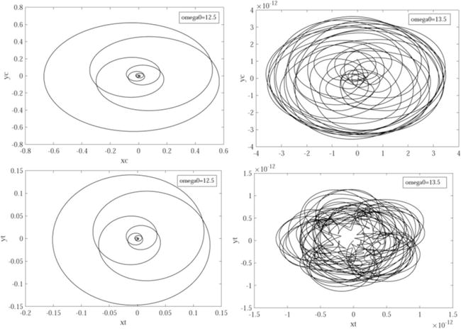
Inertia properties of the Top are m = 30 kg and ${\mathbf{J}}^{\prime }=diag\left(\mathrm{90,90,30}\right)$$\mathrm{kg}\cdot {\mathrm{m}}^2$. The initial configuration of the system is with the tip on the $z$-axis one unit below the origin, the centroid at the origin, and the $z^{\prime }$-axis coincident with the $z$-axis, so ${\mathbf{q}}^0={\left[0001000\right]}^{\mathrm{T}}$. The initial velocity is ${\dot{\mathbf{r}}}^0=\mathbf{0}$. The initial angular velocity in the body fixed $x^{\prime }-y^{\prime }-z^{\prime }$ reference frame is ${{\omega }^{\prime }}^0=\left[\epsilon \epsilon \omega z^0\right]$, where initial angular velocity components $\epsilon ={10}^{-12}$ about the $x^{\prime }$ and $y^{\prime }$ axes play the role of perturbations from the vertical configuration. From Eq. (38) of the Appendix, ${\dot{\mathbf{p}}}^0=0.5\mathbf{G}{\left({\mathbf{p}}^0\right)}^{\mathrm{T}}{{\omega }^{\prime }}^0$. As a check on conservation of energy, total energy is $\mathit{TE}=2{\dot{\mathbf{p}}}^{\mathrm{T}}\mathbf{G}{\left(\mathbf{p}\right)}^{\mathrm{T}}{\mathbf{J}}^{\text{'}}\mathbf{G}\left(\mathbf{p}\right)\dot{\mathbf{p}}+{\mathit{mgr}}_z$, where $r_z$ is the $z$ component of the vector $\mathbf{r}$.

General-purpose MATLAB Code 5.9 of [3] that is available for download at no cost from ResearchGate has been used to implement the manifold-based ODE formulation for this example. Simulation results in Figure 5 obtained using the fourth order Nystrom4 explicit integrator [16] with constant step size 0.001 s show the Top stabilizing at an initial angular velocity about the $z^{\prime }$-axis of approximately 13.5 rad/s. The upper plots for each initial angular velocity are $x-y$ trajectories of the centroid and the lower plots are $x-y$ trajectories of the tip. Total energy variation for this conservative system was 2e−4% over the 100 s simulation. On average, charts were algorithmically reparametrized 524 times during e5 time steps in each simulation, all due to a limit of 0.75 on the norm of $\mathbf{v}$, or once per 191 time steps. Only 0.02% of CPU time and no person effort was devoted to reparameterization.

Figure 5.

Plots of centroid and tip x-y trajectories for top on Bar.

As evidence that the formulation provides accurate results, with Tol = Btol = utol, where Btol and utol are defined in Eqs. (15) and (16), the maximum norm of error in position, velocity, and acceleration constraints over 100 s simulations are reported in Table 1. As predicted by the theory, these errors approach zero to computer precision as Tol approaches zero.

Tol	Pos constr err	Vel constr err	Acc constr err
e−6	2e−8	e−6	5e−5
e−8	2e−10	3e−8	2e−7
e−10	2e−12	2e−10	4e−9

Table 1.

Maximum norm of position, velocity, and acceleration constraint error.

7.2 Triple slider-crank

For numerical treatment of the triple slider-crank of Figure 1, the mechanism is modeled as four planar bodies, each with three generalized coordinates ${\mathbf{q}}_i={\left[r_i^{\mathrm{T}}{\phi }_i\right]}^{\mathrm{T}}$, so $\mathit{ngc}=12$. Three translational constraints, one revolute constraint, and two distance constraints are imposed, for a total of $\mathit{nhc}=10$ constraints. For simulation using the manifold-based ODE formulation, therefore, $\mathbf{B}\left(\mathbf{q}\right)$ is a $10\times 10$ matrix function of 12 generalized coordinates and $\mathbf{h}\left(\mathbf{v}\right)$ is a 10-vector function of two independent variables. The dimensionality of the formulation is thus much higher than the spatial spinning Top. Simulation using the manifold-based ODE formulation was carried out using MATLAB Code 5.7 of [3].

In order to avoid singular configurations identified in Section 2.3, a torque $\tau$ shown in Figure 1 is defined on ${\tilde{C}}_1$ and ${\tilde{C}}_3$ of Eq. (7) as

$$\tau =\frac{{\mathit{Kq}}_2}{{\left(\pi /2-|q_2|\right)}^2}$$

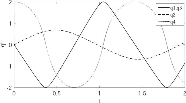
A similar torque will assure avoidance of singularities in ${\tilde{C}}_2$ and ${\tilde{C}}_4$. For purposes of simulation, parameters are selected as $K=100\mathrm{N}/\mathrm{m}$; inertia properties in the mks system are $m_1=2,J_1=1,m_2=10,J_2=10,m_3=2,J_3=1,m_4=2$ and $J_4=1$; and initial conditions in ${\tilde{C}}_3$ are $q_1^0=0,q_2^0=0,q_3^0=2,q_4^0=2,{\dot{q}}_1^0=-6,{\dot{q}}_2^0=2,{\dot{q}}_3^0=-6,{\dot{q}}_4^0=0$. For simulation in ${\tilde{C}}_1$, the same data are used, except with the initial condition $q_3^0=0$.

Simulation in ${\tilde{C}}_3$ is carried out using the fourth order Nystrom4 explicit integrator and a second order trapezoidal implicit integrator [3]. Identical results were obtained for each integrator and, since the ODE is not stiff, the Nystrom4 integrator was used to carry out multiple simulations. Plots of $q_i$, $i=\mathrm{1,2,3,4}$ for the simulation in ${\tilde{C}}_3$ are shown in Figure 6. Results for simulation with initial condition $q_3^0=0$ in ${\tilde{C}}_1$ are shown in Figure 7. In both simulations, trajectories are confined to the component in which they were initiated, consistent with the theory.

Figure 6.

Triple slider-crank simulation in ${\tilde{C}}_3$.

Figure 7.

Triple slider-crank simulation in ${\tilde{C}}_1$.

In each simulation, charts were algorithmically reparametrized 6 times during 2000 time steps of simulation, or once per 333 time steps. Only 0.068% of CPU time and no person effort was devoted to reparameterization.

As evidence that the formulation provides accurate results, with Tol = Btol = utol, where Btol and utol are defined in Eqs. (15) and (16), the maximum norm of error in position, velocity, and acceleration constraints over three simulations in ${\tilde{C}}_3$ are reported in Table 2. As predicted by the theory, these errors approach zero to computer precision as Tol approaches zero.

Tol	Pos constr err	Vel constr err	Acc constr err
e−6	6e−12	9e−7	9e−6
e−8	5e−12	8e−9	8e−8
e−10	7e−15	7e−11	4e−10

Table 2.

Maximum norm of position, velocity, and acceleration constraint error.

8. Conclusions

Topological properties of Euclidean space that are summarized in Section 2 provide a rich foundation for differentiable manifold-based mechanical system kinematics and dynamics. Topological vector space attributes of Euclidean space are shown to be adequate for systematic treatment of mechanical system dynamics, without the need for more abstract theories of differential geometry that do not represent properties of mechanical system kinematics in Euclidean space. In the Euclidean setting, with modest results from multivariable calculus, local parameterization of the regular configuration space is carried out to constructively define a differentiable manifold structure that leads to Lagrange multiplier-free, well-posed ODE of mechanical system dynamics on maximal, singularity free, path connected components of regular configuration space.

Two examples demonstrate that error control is maintained for all three forms of holonomic kinematic constraint and that reparameterizations required in mechanical system dynamic simulation are algorithmically implemented, without person interaction, and require only approximately 0.02% of simulation CPU time. This suggests that alarm expressed in the engineering literature regarding the onerous overhead and complexity of reparameterization on a manifold is unwarranted. In fact, for spatial system simulation, since global orientation representation with any set of three parameters is impossible, numerous reparameterizations are unavoidable.

With rotation of an orthogonal $x^{\prime }-y^{\prime }-z^{\prime }$ frame by a counter-clockwise angle $\chi$ about a unit vector $\mathbf{u}$ in the orthogonal $x-y-z$ frame, four Euler parameters $e_0≔cos\left(\chi /2\right)$ and $\mathbf{e}≔sin\left(\chi /2\right)\mathbf{u}$ define the orthogonal orientation transformation matrix from the $x^{\prime }-y^{\prime }-z^{\prime }$ frame to the $x-y-z$ frame as [3].

$$\mathbf{A}=\left(e_0^2-{\mathbf{e}}^{\mathrm{T}}\mathbf{e}\right)\mathbf{I}+2{\mathbf{ee}}^{\mathrm{T}}+2e_0\tilde{\mathbf{e}}$$E36

where $\tilde{\mathbf{e}}=\left[\begin{array}{ccc}0& -e_3& e_2\\ e_3& 0& -e_1\\ e_2& e_1& 0\end{array}\right]$. The 4-vector of Euler parameters is defined as $\mathbf{p}={\left[e_0{\mathbf{e}}^{\mathrm{T}}\right]}^{\mathrm{T}}$. A direct calculation yields ${\mathbf{p}}^{\mathrm{T}}\mathbf{p}=e_0^2+{\mathbf{e}}^{\mathrm{T}}\mathbf{e}={cos}^2\left(\chi /2\right)+{sin}^2\left(\chi /2\right){\mathbf{u}}^{\mathrm{T}}=1$, where the condition that u is a unit vector has been used. This yields the identity,

$${\mathbf{p}}^{\mathrm{T}}\mathbf{p}=1$$E37

which is called the Euler parameter normalization constraint.

Numerous identities and derivative relationships involving Euler parameters are due to the quadratic form of terms in the orientation transformation matrix of Eq. (36), as functions of Euler parameters [3]. Defining the $3\times 4$ matrices $\mathbf{E}\left(\mathbf{p}\right)≔\left[-\mathbf{e}\tilde{\mathbf{e}}+e_0\mathbf{I}\right]$ and $\mathbf{G}\left(\mathbf{p}\right)≔\left[-\mathbf{e}-\tilde{\mathbf{e}}+e_0\mathbf{I}\right]$, direct manipulation yields

$$\mathbf{A}\left(\mathbf{p}\right)=\mathbf{E}\left(\mathbf{p}\right)\mathbf{G}{\left(\mathbf{p}\right)}^{\mathrm{T}}$$

Carrying out the matrix products indicated shows that

$$\begin{array}{c}\mathbf{E}\left(\mathbf{p}\right)\mathbf{p}=\mathbf{0}=\mathbf{G}\left(\mathbf{p}\right)\mathbf{p}\\ \mathbf{G}\left(\mathbf{p}\right)\mathbf{G}{\left(\mathbf{p}\right)}^{\mathrm{T}}=\mathbf{I}=\mathbf{E}\left(\mathbf{p}\right)\mathbf{E}{\left(\mathbf{p}\right)}^{\mathrm{T}}\end{array}$$

where the last relation holds only if $\mathbf{p}$ is normalized. Angular velocity, represented in the body-fixed $x^{\prime }-y^{\prime }-z^{\prime }$ frame, is related to Euler parameters and their derivatives as follows:

$$\begin{array}{c}{\omega }^{\prime }=2\mathbf{G}\left(\mathbf{p}\right)\dot{\mathbf{p}}\\ \dot{\mathbf{p}}=\frac{1}{2}{\mathbf{G}}^{\mathrm{T}}\left(\mathbf{p}\right){\omega }^{\prime }\end{array}$$E38

Finally, the derivative of $\mathbf{A}\left(\mathbf{p}\right){\mathbf{a}}^{\prime }$ with respect to $\mathbf{p}$, with ${\mathbf{a}}^{\prime }$ constant, is

$${\left(\mathbf{A}\left(\mathbf{p}\right){\mathbf{a}}^{\prime }\right)}_{\mathbf{p}}=\mathbf{B}\left(\mathbf{p},{\mathbf{a}}^{\prime }\right)=2\left[\left(e_0\mathbf{I}+\tilde{\mathbf{e}}\right){\mathbf{a}}^{\prime }\mathbf{e}{{\mathbf{a}}^{\prime }}^{\mathrm{T}}-\left(e_0\mathbf{I}+\tilde{\mathbf{e}}\right){\tilde{\mathbf{a}}}^{\prime }\right]$$E39

References

1.Petzold LD. Differential/algebraic equations are not ODE’s. SIAM Journal of Scientific and Statistical Computing. 1982;3(3):367-384
2.Warner FE. Foundations of Differentiable Manifolds and Lie Groups, Graduate Texts in Mathematics. New York: Springer; 1983
3.Haug EJ. Computer-Aided Kinematics and Dynamics of Mechanical Systems, Modern Methods. 3rd ed. Vol. II. Berlin: ResearchGate; 2022. Available from: www.researchgate.net
4.Strang G. Liner Algebra and its Applications. 2nd ed. New York: Academic Press; 1980
5.Haug EJ. Extension of Maggi and Kane equations to holonomic dynamic systems. Journal of Computational and Nonlinear Dynamics. 2018;13:121003
6.Bauchau OA, Laulusa A. Review of contemporary approaches for constraint enforcement in multibody systems. Journal of Computational and Nonlinear Dynamics. 2008;3:011005
7.Laulusa A, Bauchau OA. Review of classical approaches for constraint enforcement in multibody systems. Journal of Computational and Nonlinear Dynamics. 2008;3:011004
8.Blajer W. Methods for constraint violation suppression in the numerical simulation of constrained multibody systems-a comparative study. Computer Methods in Applied Mechanics and Engineering. 2011;200:1568-1576
9.Marques F, Souto AP, Flores P. On the constraints violation in forward dynamics of multibody systems. Multibody System Dynamics. 2017;39:385-419
10.Stuelpnagel J. On the parametrization of the three-dimensional rotation group. SIAM Review. 1964;6(4):422-430
11.Pars LA. A Treatise on Analytical Dynamics, Reprint by Ox Bow Press (1979). Conn: Woodbridge; 1965
12.Atkinson KE. An Introduction to Numerical Analysis. 2nd ed. New York: Wiley; 1989
13.Tseng F-C, Ma Z-D, Hulbert GM. Efficient numerical solution of constrained multibody dynamics systems. Computer Methods in Applied Mechanics and Engineering. 2003;192:439-472
14.Garcia de Jalon J, Callejo A, Hidalgo AF. Efficient solution of Maggi’s equations. Journal of Computational and Nonlinear Dynamics. 2012;7:021003
15.Teschl G. Ordinary Differential Equations and Dynamical Systems. Providence, Rhode Island: American Math Society; 2012
16.Hairer E, Norsett SP, Wanner G. Solving Ordinary Differential Equations I: Nonstiff Problems. 2nd ed. Berlin: Springer-Verlag; 1993
Written By
Edward J. Haug and Petar Pavesic
Submitted: 29 November 2022Reviewed: 02 December 2022Published: 23 January 2023
Open access peer-reviewed chapter