Analytical Description of Unified Field Theory for Electromagnetic and Gravity Fields with the Introduction of Quantized Spacetime and Zero-Point Energy

Abstract

We have previously derived the quantized Einstein’s gravity (QEG) equation using concepts of zero-point energy and quantized space times. The theory section in this chapter provides an analytical solution of the QEG equation that implies conservation of angular momentum in terms of quantized space times. Moreover, the temperature of the cosmic microwave background (CMB) emission is obtained, and the QEG equation solution results in an analytical (not numerical) derivation of a gravity wave. We have also analytically attempted to calculate every equation in terms of electromagnetic and gravity fields using the QEG equation solution. In the Results section of this chapter, we first confirmed that the CMB emission temperature agrees with measured values. Then, the analytical solution of the QEG equation resulted in most electromagnetic and gravity field laws, in addition to the analytically derived gravity wave, which agrees well with recent measurements. Moreover, calculations of energies in the basic configuration of quantized space times resulted in the rest energies of all three leptons. Considering this basic configuration is uniformly distributed everywhere in the universe, we can conclude that τ-particles or static magnetic field energy derived from the basic configuration of quantized space times is dark energy, which is also distributed uniformly in the universe.

1. Introduction

1.1 Content summary, including previous works

This paper introduces the concepts of quantized space times and zero-point energy. We have succeeded in reinforcing our previously established unified particle theory [1, 2] and provided the reason for three generations of leptons with these concepts. Furthermore, these concepts result in the quantization of Einstein’s gravity (QEG) equation, and its analytical solution imply conservation of angular momentum in terms of quantized spacetimes. This solution solves current universe problems, such as dark energy, analytical gravity waves, etc., and creates most laws and equations regarding electromagnetic and gravity fields. Electromagnetic and gravity fields are related to weak interaction, strong interaction, neutrinos, quarks, and protons because these fields are also created from the zero-point energy [1, 2], i.e., static fields. Here, we reinforce the unified field theory introduced in the previous paper and present the basic principle that the conservation of angular momentum in terms of quantized space times, i.e., both zero-point energy and quantized space times, creates most laws regarding particle physics.

1.2 Background

In our previous papers [1, 2], we succeeded in describing most electromagnetic, gravity, weak, and strong interactions using zero-point energy and quantized space times with no numerical or fitting methods. These descriptions were found to be in agreement with measurements. In another paper [3], we analytically described neutrino self-energy and their oscillations, which also agreed with measurements.

However, in these previous papers, we did not describe the following.

1. Rotations of quantized space times using the QEG equation derived in [1].

2. Comparisons with measurements that prove the existence of the proposed quantized spacetimes.

3. Our neutrino theory [3] depends on the assumption that masses of the three leptons are given.

4. The definition of dark energy in view of particle physics.

Regarding the three lepton masses, we succeed in obtaining their values in the present chapter from the basic configuration of quantized space times. This result is important because our presented concept of quantized space times is certified by measurements. Additionally, we can conclude that the energy of this configuration of quantized space times implies dark energy because dark energy generally distributes uniformly. Furthermore, this configuration also implies that the static magnetic field energy (in GeV order) can explain recent measurements [4, 5] wherein there are static magnetic fields everywhere in the universe, even in non-macroscopic objects.

One significant point of this paper is that we succeed in obtaining the analytical (not numerical) solution of Einstein’s gravity equation. The introduction of quantized space times results in the QEG equation, which enables us to analytically solve this equation. The resultant facts from this analytical solution are as follows.

1. The temperature for cosmic microwave background (CMB) emission is predicted and agrees with measurements.

2. The gravitational wave, which has previously been calculated only using numerical methods, is calculated analytically.

3. With the concept of quantized space times and the QEG equation solution, the conservation of angular momentum of quantized spacetimes creates most laws in electromagnetism and gravity. That is, the unified field theory of particle physics is now reinforced with our previous papers [1, 2].

Here, let us consider the problems in the current standard big-bang model.

1. The current model cannot explain acceleration expansion in the universe with quantity [6].

2. There is a light-element problem in the standard model. The prediction for the amount of Li (lithium) by the standard big-bang model does not agree well with recent measurements [7].

3. As mentioned earlier, CMB emissions are well described without the standard big-bang model.

4. The most serious problem with the standard big-bang model is that it must assume infinite energy in the universe considering the singularity. This assumption is strong in all general physics equations because all physics equations generally form under conservation of energy.

5. The big-bang model does not describe dark energy, which is clarified by the current study. However, this paper claims that this energy is merely a well-known particle that obeys general gravitational law. Therefore, this paper claims that dark energy, which exhibits repulsive forces, does not exist.

In short, the standard big-bang model cannot describe recent cosmology problems and is not supported by measurements. In particular, the abovementioned “Li problem” is serious. Therefore, a new model has been recently pursued by other researchers.

1.3 Summary of the significance of the present paper

We have succeeded in confirming the existence of the basic configuration of quantized spacetimes, and the concepts of quantized space times and zero-point energy have resulted in an analytical solution of Einstein’s gravity equation. This implies conservation of the angular momentum of quantized space times. This solution creates most electromagnetic and gravity field laws and equations. In our previous papers [1, 2], weak interaction, strong interaction, and particle fields are well described using only the concepts of zero-point energy and quantized space times. Therefore, we now address an important principle: most physical fields and their laws are created only by conservation of angular momentum in terms of quantized space times, i.e., zero-point energy with the introduction of quantized space times.

This paper was also able to obtain the reason why leptons and neutrinos have three generations, which has been a puzzle since particle physics was established. Additionally, the main problems in cosmology have been solved here without the standard big-bang model. In particular, the gravity wave was obtained analytically.

2. Theory

2.1 Review of the concepts of quantized spacetimes and Einstein’s gravity equation

2.1.1 Quantized spacetime concept

We begin with the result of the Dirac equation, which implies that a photon creates an electron and a positron:

$$ħ{\omega }_0=2m_e{c}^2,$$E1

where ω_0,m_e, and c denote a constant angular frequency, the mass of an electron, and the speed of light, respectively. This equation can be interpreted as

$$\frac{1}{2}ħ{\omega }_0=m_e{c}^2$$E2

and produces the minimum quantized length, ${\lambda }_0$, and time t₀ in terms of a space time:

$${\lambda }_0=\frac{ħ}{2m_{e}c}$$E3

and

$$t_0=\frac{ħ}{2m_e{c}^2}.$$E4

We derive a more general constant quantized space-time length and time:

$${\lambda }_c={\lambda }_0\sqrt{1-\frac{v^2}{c^2}}$$E5

and

$$t_c=t_0\sqrt{1-\frac{v^2}{c^2}}.$$E6

We consistently assume that the above length (5) and time (6) are minima, thus, they cannot be divided further. As discussed later, it was found that these concepts are supported by measurement.

In Eq. (2), the left-hand side is identical for the zero-point energy in the harmonic oscillator Hamiltonian:

$$H=\left(n+\frac{1}{2}\right)ħ{\omega }_0.$$E7

As every quantum field theory argues, the first term in Eq. (7) implies alternating current electromagnetism. However, the second term, called zero-point energy (neglected in quantum field theory), is more important because of direct current (DC) electromagnetism. Note that we will report that the first term creates Maxwell’s time-dependent equations in view of different approaches from quantum field theory.

Figure 1 shows a schematic of the basic configuration of quantized space times. Two quantized space times, in terms of an electric field, are rotating with velocity v. Each quantized space time, in terms of an electric field, has embedded up- and down-spin electrons (this will become important when considering the creation of a μ-particle). Note that it is necessary to distinguish these embedded electrons from real body electrons. By rotations of embedded electrons, i.e., the rotations of the two quantized space times, another quantized space time is induced in terms of a magnetic field. This magnetic field accompanies the concept of flux (defined in the central circle in Figure 1), that is, another quantized space time whose radius is the same as λ_c. Therefore, it is very important to distinguish the two quantized space times as:

1. a quantized space time accompanying an embedded electron in terms of an electric field and

2. a quantized space time induced in terms of a magnetic field.

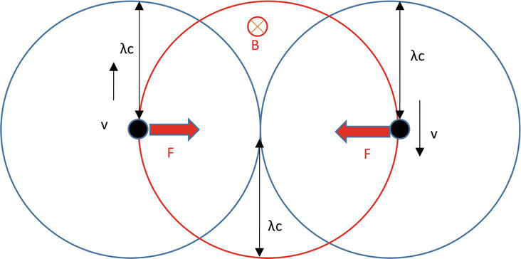
Figure 1.

Diagram of the basic configuration of quantized space times.

The radius of the quantized time space is ${\lambda }_c$, which is determined using the Dirac equation and Lorentz contraction. For details, refer to our previous paper [1]. The black dot denotes an embedded electron, which rotates with velocity v. The force F is generated as a result of magnetic field generation (the Lorentz force). Note that the magnetic flux is defined in the central circle. As discussed in our various previous papers, when the relative momentum in terms of two charged particles is zero, these two particles generally experience an attractive force that stems from the Lorentz force. As shown, this attractive force F is identical to an attractive gravity force, which is related to the quantization of Einstein’s gravity equation.

As will be discussed later, the energies of the two quantized space times are commonly expressed as zero-point energies. Force F is the Lorentz force originating from the static magnetic field, and it is identified by attractive gravity forces, F, from the gravitational field. This is important because gravity and the magnetic field are unified in this scale, which results in the quantized Einstein’s gravity equation. An important note is that this configuration can be described by the QEG equation solution, as will also be discussed later.

2.1.2 Quantization of Einstein’s gravity equation

According to our previous paper [1], energy relationships in terms of gravity, static magnetic field, and electric field in the scale of the quantized space times are derived as

$$u_B=-G^2\frac{1}{r^4}\frac{1}{c^2}{u}_E{\left(\frac{ħ}{2c^2}\right)}^2,u_B=u_G$$E8

where r, G, u_B, u_G, and u_E denote the distance, the gravitational constant, magnetic field energy, gravity field energy, and electric field energy, respectively. We can combine Eq. (8) with Einstein’s gravity equation because both equations include G. The existing Einstein’s equation is

$$G_{\mathit{\mu \nu }}=\frac{8\mathit{\pi G}}{c^4}{T}_{\mathit{\mu \nu }}$$E9-1

and

$$G_{\mathit{\mu \nu }}=R_{\mathit{\mu \nu }}-\frac{1}{2}R{g}_{\mathit{\mu \nu }},$$E9-2

where R_μν, T_μν, g_μν, and R denote the Riemann curvature tensor, the energy flux tensor, the metric tensor, and the Ricci tensor, respectively.

As a result of substituting G in Eq. (8), we obtain

$$G_{\mathit{\mu \nu }}=\frac{16\pi }{\mathit{cħ}}\sqrt{\frac{-u_B}{u_E}}{\lambda }_c^2{T}_{\mathit{\mu \nu }}.$$E10

Now, it is assumed that the macroscopic tensor g_μν is approximately the Minkowski tensor, g_ij, because an analytical differential cannot be defined for a quantized space time [1]. That is, it merely implies division by λ_c[1]. Similarly, the energy density is given using zero-point energy:

$$\epsilon =\frac{1}{2}\mathit{ħ\omega }/{\lambda }_c^3.$$E11

Thus, T_μν is approximated using the Minkowski tensor:

$$T_{\mathit{\mu \nu }}=\epsilon g_{\mathit{ij}}.$$E12

Considering the above, Einstein’s gravitational equation is transformed to

$$R_{\mathit{\mu \nu }}=\left(\frac{16\pi }{\mathit{cħ}}\sqrt{\frac{-u_B}{u_E}}\frac{\left|u_G\right|}{{\lambda }_c}+\frac{1}{2}R\right)g_{\mathit{ij}}.$$E13

The energy of a quantized space time regarding a magnetic field is given as the zero-point energy:

$$\left|u_G\right|=\frac{1}{2}\mathit{ħ\omega }.$$E14

Assuming the Ricci tensor, ½R, to be substantially smaller than the first term, we obtain

$$R_{\mathit{\mu \nu }}=\left(\frac{16\pi }{\mathit{cħ}}\sqrt{\frac{-u_B}{u_E}}\frac{1}{{\lambda }_c}\frac{1}{2}\mathit{ħ\omega }\right)g_{\mathit{ij}}.$$E15

Moreover, considering Eq. (8), the ratio u_B/u_E in Eq. (15) is obtained:

$$u_B=-G^2\frac{1}{r^4}\frac{1}{c^2}{u}_E{\left(\frac{ħ}{2c^2}\right)}^2=-G^2\frac{1}{{\lambda }_c^4}\frac{1}{c^2}{u}_E{\left(\frac{ħ}{2c^2}\right)}^2.$$E16

Considering this, we obtain conclusively

$$R_{\mathit{\mu \nu }}=\left(G\frac{8\pi }{c^4}\frac{1}{{\lambda }_c^3}\frac{1}{2}\mathrm{ħ}\omega \right)g_{\mathit{ij}}.$$E17

2.2 Zero-point energy in quantized spacetime for gravity or magnetic fields

Let us estimate the zero-point energy in terms of a magnetic or gravity field as well as in terms of an electric field concerning quantized space time. Here we consider energy level $\left|\Delta \right|$from special relativity:

$$\left|\Delta \right|=\frac{m_e{c}^2}{\sqrt{1-\frac{v^2}{c^2}}}.$$E18

This energy level is located at the middle position within the band gap of the vacuum, i.e., the energy gap is $2\left|\Delta \right|$. If $v\ne 0$ in Eq. (18), $2\left|\Delta \right|$ is produced by the product of both the fine-structure constant, α, and zero-point energy:

$$2\left|\Delta \right|=\frac{1}{2}\mathit{ħ\omega }\times \alpha .$$E19

This fact will be proved while discussing CMB here or can be referenced in the literature [8]. Note that if v = 0 in Eq. (18), this equation for $\left|\Delta \right|$ implies the zero-point energy in terms of an electric field, which is related to Eq. (2).

Conversely, v in Eq. (18) is assumed to be the critical velocity, v_c, for an electron. That is, an electron has a maximum velocity v_c less than the speed of light c when largely accelerated. According to our previous papers [1, 3], an electron can accompany an e-neutrino and, thus, the e-neutrino speed is equal to the critical velocity of an electron. Therefore, v = v_c is substituted in Eq. (18) by 0.994c [1, 3]. Using Eq. (19), the calculated zero-point energy for the magnetic or gravity field then becomes

$$\frac{1}{2}\mathit{ħ\omega }=\frac{2}{\alpha }\left|\Delta \right|=1.23\times {10}^9\mathrm{eV}.$$E20

This value agrees with the measurement of a τ-particle [9].

In summary, the zero-point energy is related to special relativity energy, Eq. (18), where v = 0 implies the rest energy of an electron and is related to the quantized space time in terms of an electric field. While v in Eq. (18) is the v_c for an electron, the zero-point energy in Eq. (19) implies quantized space time in terms of magnetic or gravity fields.

2.3 Three generations of lepton

2.3.1 Collapse of the basic configuration of quantized spacetimes

Figure 2 schematically indicates how the magnetic or gravity field in a quantized spacetime (i.e., the combination of two embedded electrons in two quantized space–times) collapses. Each quantized space time in terms of magnetic or gravity fields has a torque property whose moment corresponds to the magnetic field vector.

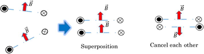
Figure 2.

Schematic wherein two quantized space times in terms of a magnetic or gravity field interact with each other and how these quantized space times collapse. This figure was cited from [10].

First, a quantized space time in terms of magnetic field has a torque property whose moment corresponds to its magnetic field vector. The superposition case in this figure is such that the two magnetic field vectors are maximally strengthened. An important case is their cancelation with each other wherein the quantized space times in terms of a magnetic field collapse.

From torque properties, a larger magnetic field is generated if two magnetic field vectors of two quantized space times in terms of a magnetic field take the same direction. Generally, this maximum superposition occurs in the location of the universe at which the gravity field becomes extremely strong. On the contrary, however, if two magnetic field vectors of two quantized space times in terms of the magnetic field take reverse directions, the net magnetic field vanishes. The magnetic field energy is converted to τ-particles while μ-particle energy comes from the spin interaction of two electrons embedded in quantized space times in terms of the electric field. In this way, a quantized space time in terms of a magnetic or gravity field collapses even though the combination energy of two embedded electrons in two quantized space times is quite large [3]. This fact results in the creation of τ- and μ-particles, as discussed later.

2.3.2 Masses of μ- and τ-particles from the basic configuration of quantized spacetimes

This paper claims that the masses of the three generations of leptons stem from the abovementioned collapse of the basic configuration of quantized space times. As a result of the collapse, three energies are generated from collapsed quantized space times. Based on Figure 1, we claim the following points.

1. The combination energy between two embedded electrons in quantized space times in terms of electric field, i.e., the magnetic field (gravity field) energy in a quantized space time, is converted. This energy corresponds to the remaining energy of the τ-particle.

2. Each embedded electron in two quantized space times, which take rotations and induce the magnetic field energy in quantized space time, have interactions in terms of spins (up and down). This interaction is converted to the remaining energy of the μ-particle.

3. Embedded electrons in Figure 1 automatically gain real bodies.

In the Results section, actual calculations illustrating these points will be conducted.

2.4 Analytical solution to the quantized Einstein’s gravity equation

We now consider the quantized Einstein’s gravity (QEG) equation.

$$R_{\mathit{ij}}=\frac{8\mathit{\pi G}}{c^4}\frac{\frac{1}{2}\mathit{ħ\omega }}{{\lambda }_c^3}{g}_{\mathit{ij}},$$E21

where the Minkowski tensor, $g_{\mathit{ij}}$, is given by

$$g_{\mathit{ij}}=\left(\begin{array}{cccccc}& -1& & & & 0\\ & & -1& & & \\ & & & -1& & \\ 0& & & & +1& \end{array}\right)$$E22

This QEG equation requires a specific form of the Riemann curvature tensor, $R_{\mathit{ij}}$, for the following reasons.

1. Because $g_{\mathit{ij}}$ is a diagonal matrix, $R_{\mathit{ij}}$ is a diagonal matrix considering Eq. (21).

2. The QEG equation must automatically express Lorentz conservation and does not include this conservation as a condition.

3. $R_{\mathit{ij}}$ is a covariance tensor. Thus, it must be composed by the direct product of position vector $k$:

$$k=x{e}^1+y{e}^2+z{e}^3+\mathit{ict}{e}^4,$$E23

where i in the fourth term denotes the imaginary unit.

$$k\times k\to R_{\mathit{ij}},$$E24

where the symbol × implies the direct product of the vectors in this paper.

Since

$$e^i\bullet e^j={\delta }^{\mathit{ij}},$$E25

$$R_{\mathit{ij}}=\left(\begin{array}{cccccc}& x^2& & & & 0\\ & & y^2& & & \\ & & & z^2& & \\ 0& & & & -{\left(\mathit{ct}\right)}^2& \end{array}\right)$$E26

In the QEG equation, Eq. (21) takes the trace, Tr, to form Lorentz conservation:

$$x^2+y^2+z^2-{\left(\mathit{ct}\right)}^2=\left(-2\right)\frac{8\mathit{\pi G}}{c^4}\frac{\frac{1}{2}ħ{\omega }_i}{{\lambda }_c^3}.$$E27

According to Eq. (27), Lorentz conservation is automatically presented. In the derived equation, time t should be considered a period,

$$r_i^2\equiv x^2+y^2=\left(-2\right)\frac{8\mathit{\pi G}}{c^4}\frac{\frac{1}{2}ħ{\omega }_i}{{\lambda }_c^3}+{\left(c\frac{2\pi }{\omega }\right)}^2-z^2,$$E28

where r_i implies the radius of rotation at each location indexed by i, and we assume cylindrical coordinates. Note that r_i depends on the values of variable z. Moreover, variable angular frequency ω was introduced because time t implies a period. As will be described later, the derived equation implies that z gives an anisotropic property. We will see that this solution of the QEG equation describes both electromagnetism and gravity fields well.

Considering Eqs. (21), (22), and (26), each position and time variable, x, y, z, and t, are not independently defined. Thus, the Eq. (21) obtains its meaning only when the trace of both sides is considered. This fact is important because we claim that moving (rotating) space time exists. That is, the mathematical metrics in terms of Cartesian geometry are an approximated concept in a vacuum. This can be understood by considering an analogy that, while a rigid body has metrics on it like a length of a line, the area of a square, etc., at the microscopic scale of the rigid body, many thermally fluctuated lattices (phonons) exist and imply that the mathematical metrics on the rigid body are not formed at the microscopic scale.

2.5 Cosmic microwave background (CMB)

First, let us consider the analytical solution of the QEG equation again:

$$r_i^2\equiv x^2+y^2=\left(-2\right)\frac{8\mathit{\pi G}}{c^4}\frac{\frac{1}{2}ħ{\omega }_i}{{\lambda }_c^3}+{\left(c\frac{2\pi }{\omega }\right)}^2-z^2.$$E29

Index i is associated with both $r_i$ and $\frac{1}{2}ħ{\omega }_i$. Note that here we assume z = 0, resulting in

$$r_i^2\equiv \left(-2\right)\frac{8\mathit{\pi G}}{c^4}\frac{\frac{1}{2}ħ{\omega }_i}{{\lambda }_c^3}+{\left(c\frac{2\pi }{\omega }\right)}^2.$$E30

Because r_i should be considered a macroscopic variable of radius, the first term of the right-hand side (i.e., the zero-point energy having index i) should be neglected. As a result, considering the area of a circle, the macroscopic variable radius r appears and thus a unique angular frequency is derived as

$$\omega =\frac{\sqrt{4\pi }c}{r}.$$E31

Next, the angular frequency ω in Eq. (31) are substituted into the Prank emission, ${\alpha }_T$, Eq. (32):

$${\alpha }_T=\frac{1}{{\pi }^2}\frac{\mathit{ħ\omega }/c^2}{\mathit{exp}\left(\frac{\mathit{ħ\omega }}{k_{B}T}\right)-1},$$E32

where T and k_B denote the temperature and the Boltzmann constant, respectively. When the exponential function in Eq. (32) becomes e⁻¹, the following equation holds:

$$\frac{k_B{T}_{0}r}{ħ\sqrt{4\pi }c}=1.$$E33

In Eq. (33), temperature T₀ implies one Prank emission. We claim that a CMB photon is derived from the energy gap, which fluctuates in the energy level of the vacuum [3] and is related to the e-neutrino self-energy. That is, considering that r in Eq. (33) is the wavelength of a photon, this wavelength can be derived from fluctuations in the vacuum energy level.

Figure 3 shows the iteration wherein photons are absorbed or emitted to or from the energy gap, respectively. This implies that CMB photons are created and absorbed everywhere in the universe, and thus, we claim that CMB photons are not the source of birth of our universe in terms of the big-bang.

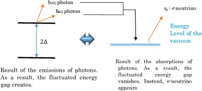
Figure 3.

Schematic representation of creation and absorption of CMB photons through the neutrino energy gap. This figure was cited from [10]. The left-hand-side panel indicates the creation of the energy gap, which fluctuates in the vacuum energy level. An energy gap is created by emission of photons from the vacuum energy level. This created energy gap is essentially equal to the self-energy of an e-neutrino. The right-hand-side panel shows the disappearance of the energy gap by absorption of photons; a real body of an e-neutrino is emitted. As mentioned in our previous paper [3], an energy gap is again created at the energy level of the vacuum according to the BCS ground state because of many-body interactions of the basic configuration of quantized space times. The left-hand and right-hand panels occur everywhere in the universe locally with iterations. Thus, the creation and absorption of photons in terms of CMB arise everywhere and the CMB source is not the birth of the universe (i.e., the big-bang).

In the Results section, the actual calculation of the phenomena discussed above will be conducted using e-neutrino self-energy.

2.6 Analytical derivation of the gravity wave

In the QEG equation solution,

$$r_i^2=x^2+y^2=\frac{-16\mathit{\pi G}}{c^4}\frac{\frac{1}{2}\mathrm{ħ}{\omega }_i}{{\lambda }_c^3}+{\left(c\frac{2\pi }{\omega }\right)}^2-z^2,$$E34

$r_i=0$ is a condition of the generation of gravity waves. Note that index i is arbitrary. The condition of the generation of gravity waves implies that previous rotations cease everywhere. That is, macroscopic rotation ceased [11, 12].

Depending on z, variable angular frequency ω is varied. The center of the previous rotation is considered in this case and in cylindrical coordinates. That is, z = 0 is assumed. This also implies that the maximum is considered. For a secondary condition, the zero-point energy is converted to a photon by the product of the fine-structure constant, α, because it is needed to convert the energy level to an energy gap. When the uncertainty relation is introduced, an ω equation dependent on Δt is derived:

$$\frac{1}{2}\mathrm{ħ}{\omega }_i\to \frac{1}{2}\mathrm{ħ}{\omega }_i\alpha =n\mathrm{ħ}\omega =\mathrm{ħ}\left(\mathit{n\omega }\right)=\left|\Delta \right|$$E35

and

$$\left|\Delta \right|\times \mathit{\Delta t}\approx ħ.$$E36

Considering Eq. (35), $\omega \to \mathit{n\omega }$ and

$${\left(c\frac{2\pi }{\mathit{n\omega }}\right)}^2=\frac{16\mathit{\pi G}}{c^4}\frac{1}{{\lambda }_c^3}\left|\Delta \right|$$E37

and

$${\left(c\frac{2\pi }{\mathit{n\omega }}\right)}^2\mathit{\Delta t}=\frac{16\mathit{\pi G}}{c^4}\frac{1}{{\lambda }_c^3}ħ.$$E38

In this equation, the distributed relationship regarding λ_c is employed:

$${\left(\mathit{n\omega }\right)}^5=\frac{\pi c^9}{4G}\frac{1}{ħ}\mathit{\Delta t}.$$E39

Moreover, quantum number n is defined as

$$\sum _n{t}_0\equiv 1\left[s\right],$$E40-1

That is,

$$n{t}_0\equiv 1.$$E40-2

Next, strain h_max is considered:

$$h_{\mathit{max}}=\frac{\mathit{\delta L}}{\frac{L}{2}}.$$E41

This definition is translated to

$$h_{\mathit{max}}=\frac{{\lambda }_c}{L/2},$$E42

where

$${\lambda }_c=c{t}_c,$$E43-1

$$t_c=t_0\sqrt{1-\frac{v^2}{c^2}},$$E43-2

and

$$v=v_c=0.994c.$$E43-3

As mentioned in Section 2.2, v_c is the critical speed of an electron and is equal to that of an e-neutrino. Therefore, this expression implies consideration of quantized space times in terms of gravity (magnetic) fields.

With

$$\frac{L}{2}=\mathit{c\Delta t}$$E44

we have

$$h_{\mathit{max}}=\frac{t_c}{\mathit{\Delta t}}$$E45

and the chirp signal is given by

$$u_p=\frac{t_c}{\mathit{\Delta t}}\mathit{cos}\left(\omega t_{00}\right),$$E46

where $t_{00}$ is defined as the constant 1[s] because ω is a variable dependent on Δt. The chirp signal will be further discussed in the Results section.

2.7 Unified field picture in terms of electromagnetic and gravity fields by rotations of quantized spacetimes

The solution of the QEG equation is again given as

$$r_i^2=x^2+y^2={\left(c\frac{2\pi }{\omega }\right)}^2-\frac{16\mathit{\pi G}}{c^4}\frac{1}{{\lambda }_c^3}\frac{1}{2}ħ{\omega }_i,$$E47

where z = 0 is assumed.

As mentioned earlier, this equation implies quantized time-space rotation.

2.7.1 The case of direct current

2.7.1.1 General notation

Eq. (47) creates every equation regarding electromagnetism and Newtonian gravity. To show this, λ_c should first be canceled and later we consider general fields. We assume that electric and magnetic fields only in a quantized space time have energies

$$\frac{1}{2}ħ{\omega }_i=\frac{1}{2}{\epsilon }_0{E}_i^2{\lambda }_c^3$$E48-1

and

$$\frac{1}{2}ħ{\omega }_i=\frac{B_i^2}{2{\mu }_0}{\lambda }_c^3,$$E48-2

respectively. Concerning gravity, in the Section 2.2, we derived the zero-point energy in terms of the gravity field:

$$\frac{1}{2}ħ{\omega }_i=\frac{2}{\alpha }\left|\Delta \right|=\frac{2}{\alpha }\frac{m_e{c}^2}{\sqrt{1-\frac{v^2}{c^2}}}.$$E48-3

Furthermore, the general wave function is considered:

$$\int {\left|\psi \right|}^2\mathit{dv}={\left|{\psi }_i\right|}^2{\lambda }_c^3=1.$$E48-4

Note that the differential and integral become merely division and product, respectively, in the quantized space time [1].

Each of the above equations is substituted into Eq. (47) and the general electric, magnetic, and gravity field equations are derived as follows:

$$r_i^2={\left(c\frac{2\pi }{\omega }\right)}^2-\frac{16\mathit{\pi G}}{c^4}\frac{1}{2}{\epsilon }_0{E}_i^2,$$E49-1

$$r_i^2={\left(c\frac{2\pi }{\omega }\right)}^2-\frac{16\mathit{\pi G}}{c^4}\frac{B_i^2}{2{\mu }_0},$$E49-2

and

$$r_i^2={\left(c\frac{2\pi }{\omega }\right)}^2-\frac{16\mathit{\pi G}}{c^4}{\left|{\psi }_i\right|}^2\frac{2}{\alpha }\frac{m_e{c}^2}{\sqrt{1-\frac{v^2}{c^2}}},$$E49-3

respectively.

2.7.1.2 Derivation of each Poisson equation

The Poisson equations can be obtained in terms of electrostatic, vector, and gravity potentials based on the results obtained in the previous section.

First, consider the Poisson equation in terms of electrostatic potential:

$$r_i^2={\left(c\frac{2\pi }{\omega }\right)}^2-\frac{16\mathit{\pi G}}{c^4}\frac{1}{2}{\epsilon }_0{E}_i^2.\left(\text{49‐1}\right)$$

If the first term is neglected,

$$r_i\equiv {\lambda }_c.$$E50

Thus,

$$\frac{1}{2}{\epsilon }_0\frac{E_i^2}{{\lambda }_c^2}=\frac{-c^4}{16\mathit{\pi G}}.$$E51-1

In Eq. (51-1), division by λ_c must be translated to the normal differential to express the mathematic equation. That is, the differential is revived [1]:

$$\frac{1}{2}{\epsilon }_0\frac{{\mathit{dE}}_i^2}{d{r}^2}=\frac{-c^4}{16\mathit{\pi G}}.$$E51-2

Thus,

$${\epsilon }_0{E}_r\frac{d{E}_r}{\mathit{dr}}\frac{1}{{\lambda }_c}=\frac{-c^4}{16\mathit{\pi G}}.$$E52

Considering the concept of quantized space times:

$$r=n{\lambda }_c,$$E53

and

$$n{E}_{r0}\frac{d{E}_r}{\mathit{dr}}\frac{1}{r}=\frac{-1}{{\epsilon }_0}\frac{c^4}{16\mathit{\pi G}}.$$E54

Introducing the electrostatic potential Φ, we have

$$E_r=\frac{-\mathit{d\Phi }}{\mathit{dr}}$$E55

and

$$\frac{-d^2\Phi }{d{r}^2}=\frac{-1}{{\epsilon }_0}\frac{c^4}{16\mathit{\pi G}}\frac{1}{n{E}_{r0}}r.$$E56

Herein, the following relation is assumed:

$$E_{r0}=-v{B}_{z0},$$E57

where v implies an arbitrary and rotational velocity, not the speed of light c, and Eq. (56) becomes

$$\frac{d^2\Phi }{d{r}^2}=\frac{-1}{{\epsilon }_0}\frac{c^4}{16\mathit{\pi G}}\frac{1}{v}\frac{1}{B_{z0}}\frac{1}{n}r.$$E58

Considering the cyclotron angular frequency,

$${\omega }_c=\frac{e{B}_{z0}}{m_e},$$E59

we have

$$\frac{d^2\Phi }{d{r}^2}=\frac{-1}{{\epsilon }_0}\frac{c^4}{16\mathit{\pi G}}\frac{1}{v}\frac{e}{m_e{\omega }_c}\frac{1}{n}r.$$E60

Or, using

$$v=r{\omega }_c,$$E61

we obtain

$$\frac{d^2\Phi }{d{r}^2}=\frac{-1}{{\epsilon }_0}\frac{c^4}{16\mathit{\pi G}}\frac{e}{m_e{\omega }_c^2}\frac{1}{n}.$$E62

Next, we consider the Poisson equation in terms of vector potential.

Similar to the case of an electric field and using Eq. (49-2), we obtain

$$B_z\frac{d{B}_z}{d{r}^2}=-{\mu }_0\frac{c^4}{16\mathit{\pi G}}$$E63

and

$$B_z\frac{d{B}_z}{\mathit{dr}}\frac{1}{{\lambda }_c}=n{B}_{z0}\frac{d{B}_z}{\mathit{dr}}\frac{1}{r}=-{\mu }_0\frac{c^4}{16\mathit{\pi G}}.$$E64

Cylindrical coordinates are considered in this case and, thus, the component of a vector potential is introduced by

$$B_z=\frac{1}{r}{A}_{\phi }.$$E65

Calculating $\frac{d{B}_z}{\mathit{dr}}$ we obtain

$$n{B}_{z0}\left(\frac{-A_{\phi }}{r^2}\right)=-{\mu }_0\frac{c^4}{16\mathit{\pi G}}r.$$E66

Thus, A_φ becomes a special dependent and division of r is transformed into the differential:

$$\frac{d^2{A}_{\phi }}{d{r}^2}={\mu }_0\frac{c^4}{16\mathit{\pi G}}\frac{1}{n{B}_{z0}}r.$$E67

With the introduction of cyclotron angular frequency ω_c we have

$$\frac{d^2{A}_{\phi }}{d{r}^2}={\mu }_0\frac{c^4}{16\mathit{\pi G}}\frac{1}{n}\frac{e}{m_e{\omega }_c}r.$$E68

Consequently,

$$\frac{d^2{A}_{\phi }}{d{r}^2}={\mu }_0\frac{c^4}{16\mathit{\pi G}}\frac{1}{n}\frac{e}{m_e{\omega }_c}r.$$E69

Next, we derive the Poisson equation in terms of gravity beginning with

$$r_i^2={\left(c\frac{2\pi }{\omega }\right)}^2-\frac{16\mathit{\pi G}}{c^4}{\left|{\psi }_i\right|}^2\frac{2}{\alpha }\frac{m_e{c}^2}{\sqrt{1-\frac{v^2}{c^2}}}.\left(\text{49‐3}\right)$$

The first term is neglected and $r_i\equiv {\lambda }_c$ is assumed, resulting in

$${\lambda }_c^2=\frac{-16\mathit{\pi G}}{c^4}{\left|{\psi }_i\right|}^2\frac{2}{\alpha }\frac{m_e{c}^2}{\sqrt{1-\frac{v^2}{c^2}}}.$$E70

In short,

$$1=\frac{-16\mathit{\pi G}}{c^4}\frac{{\left|{\psi }_i\right|}^2}{{\lambda }_c^2}\frac{2}{\alpha }\frac{m_e{c}^2}{\sqrt{1-\frac{v^2}{c^2}}}.$$E71-1

Then, the normal differential must be revived [1] to ensure the mathematical expression:

$$1=\frac{-16\mathit{\pi G}}{c^4}\frac{d^2{\left|{\psi }_i\right|}^2}{d{r}^2}\frac{2}{\alpha }\frac{m_e{c}^2}{\sqrt{1-\frac{v^2}{c^2}}}.$$E71-2

The following term for the potential energy for gravity,${\Phi }_G,$

$$\mathit{g\delta }\left(\overrightarrow{r}\right){\left|{\psi }_i\right|}^2\equiv {\Phi }_G,$$E72

where g is a variable and δ is the Dirac function, is introduced.

Thus,

$$\frac{d^2{\Phi }_G}{d{r}^2}=\frac{-c^4}{16\mathit{\pi G}}\frac{\alpha }{2}\frac{\sqrt{1-\frac{v_R^2}{c^2}}}{m_e{c}^2}\mathit{g\delta }\left(\overrightarrow{r}\right),$$E73

where $v\equiv v_R$ denotes the relative velocity between two charged particles because r in the Dirac function implies the relative distance between the two charged particles.

When relative velocity v_R is zero, two charged particles generally experience a strong attractive force with each other as the Lorentz force. For example, this attractive force creates a Cooper pair in high-temperature superconductors [13]. Therefore, when v_R is assumed to be zero, Eq. (73) is approximated as

$$\frac{d^2{\Phi }_G}{d{r}^2}=\frac{-1}{16\mathit{\pi G}}\frac{1}{m_e}{c}^2\mathit{g\delta }\left(\overrightarrow{r}\right).$$E74

In the above equation, g should be considered a variable. Note that $\frac{\alpha }{2}$ has meaning only when v_R is not zero but large; the above conclusive equation does not include this fine-structure constant.

Moreover,

$$\int \delta \left(\overrightarrow{r}\right)\mathit{dv}=1.$$E75

Considering Eq. (75), we take the volume integral to Eq. (74). Note that, spherical coordinates are considered in this case because r implies a relative distance. We obtain

$$\int \frac{d^2{\Phi }_G}{d{r}^2}4\pi r^2\mathit{dr}=\frac{-1}{16\mathit{\pi G}}\frac{1}{m_e}{c}^{2}g$$E76

with the left side equal to

$$\int d{\Phi }_G\frac{d}{\mathit{dr}}4\pi r^2=8\mathit{\pi r}{\Phi }_G.$$E77

Thus, we finally obtain a Newtonian equation:

$${\Phi }_G=\frac{-1}{8\pi }\frac{1}{16\mathit{\pi G}}\frac{c^2}{m_e}g\frac{1}{r}.$$E78

In the Results section, we will examine the validity of these derived Poisson equations using actual calculations.

2.7.2 Derivation in the case of alternating current

First, when the zero-point energy in the QEG equation solution is translated to a photon, the energy gap is expressed as

$$\frac{1}{2}ħ{\omega }_i\to \frac{1}{2}ħ{\omega }_i\alpha =\left|\Delta \right|=\left|E_i-E_j\right|$$E79

and the basic solution becomes

$$r_i^2={\left(c\frac{2\pi }{\omega }\right)}^2-\frac{16\mathit{\pi G}}{c^4}\frac{1}{{\lambda }_c^3}\left|E_i-E_j\right|,$$E80

where

$$\left|E_i-E_j\right|=\int \left|\frac{1}{2}{\epsilon }_0{E}_i^2-\frac{B_j^2}{2{\mu }_0}\right|\mathit{dv}=|\frac{1}{2}{\epsilon }_0{E}_i^2-\frac{B_j^2}{2{\mu }_0}|{\lambda }_c^3.$$E81

Thus,

$$r_i^2={\left(c\frac{2\pi }{\omega }\right)}^2-\frac{16\mathit{\pi G}}{c^4}|\frac{1}{2}{\epsilon }_0{E}_i^2-\frac{B_j^2}{2{\mu }_0}|.$$E82

As shown in Figure 4, Eq. (82) implies that the magnetic field energy indexed by j is dependent on the electric field energy indexed by i (here we do not consider the previously mentioned and basic configuration of quantized spacetimes). Thus, a magnetic field is induced by an electric field. If indices i and j are altered, the electric field energy becomes dependent and is induced from the magnetic field energy:

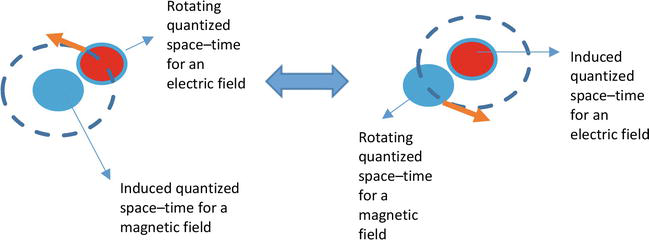
Figure 4.

Schematic of induction of quantized space times in terms of both electric and magnetic fields. This figure was cited from [10]. The left panel indicates that rotation of quantized space time for an electric field induces a quantized space time for a magnetic field. On the contrary, the right panel shows that rotation of the quantized space time for a magnetic field induces a quantized space time for an electric field.

As will be derived later, these phenomena imply the time-dependent Maxwell’s equations and indicate the process of electromagnetic wave induction.

$$r_i^2={\left(c\frac{2\pi }{\omega }\right)}^2-\frac{16\mathit{\pi G}}{c^4}|\frac{1}{2}{\epsilon }_0{E}_i^2-\frac{B_j^2}{2{\mu }_0}|\text{or}{r}_j^2={\left(c\frac{2\pi }{\omega }\right)}^2-\frac{16\mathit{\pi G}}{c^4}|\frac{-1}{2}{\epsilon }_0{E}_j^2+\frac{B_i^2}{2{\mu }_0}|.$$E83

That is, two energy levels indexed by both i and j are induced by each other and are iterated by ω. This physical picture describes the process of an electromagnetic wave and Eq. (83) implies time-dependent Maxwell’s equations.

Now we create Maxwell’s time-dependent equations based on Eq. (82):

$$\omega \to \frac{2\pi }{t_c},$$E84

$$r_i\to {\lambda }_c,$$E85

and

$${\lambda }_c^2={\left(c{t}_c\right)}^2-\frac{16\mathit{\pi G}}{c^4}\left(\frac{1}{2}{\epsilon }_0{E}^2-\frac{B^2}{2{\mu }_0}\right).$$E86

In Eq. (86), E and B are not magnitudes but components. Considering generalizations into three dimensions in view of vector analysis, these components are assumed to be arbitrary regarding any coordinates. Eq. (86) can be written as

$${\lambda }_c^2-\frac{16\mathit{\pi G}}{c^4}\left(\frac{B^2}{2{\mu }_0}\right)={\left(c{t}_c\right)}^2-\frac{16\mathit{\pi G}}{c^4}\left(\frac{1}{2}{\epsilon }_0{E}^2\right)$$E87

and from this equation we consider the following simultaneous equations:

$${\lambda }_c^2-\frac{16\mathit{\pi G}}{c^4}\left(\frac{B^2}{2{\mu }_0}\right)=\alpha .$$E88-1

and

$${\left(c{t}_c\right)}^2-\frac{16\mathit{\pi G}}{c^4}\left(\frac{1}{2}{\epsilon }_0{E}^2\right)=\alpha .$$E88-2

Eq. (88-1) becomes

$$1-\frac{16\mathit{\pi G}}{c^4}\frac{1}{2{\mu }_0}\frac{B^2}{{\lambda }_c^2}=\frac{\alpha }{{\lambda }_c^2}.$$E89

The differential must be revived and the number one is ignored to obtain:

$$\frac{-16\mathit{\pi G}}{c^4}\frac{1}{2{\mu }_0}\frac{d{B}^2}{d{r}^2}=\frac{\mathit{d\alpha }}{d{r}^2},$$E90

$$\frac{-16\mathit{\pi G}}{c^4}\frac{1}{2{\mu }_0}2B\frac{\mathit{dB}}{\mathit{dr}}\frac{1}{{\lambda }_c}=\frac{\mathit{d\alpha }}{\mathit{dr}}\frac{1}{{\lambda }_c},$$E91

and

$$\frac{-16\mathit{\pi G}}{c^4}\frac{1}{{\mu }_0}\frac{\mathit{dB}}{\mathit{dr}}B=\frac{\mathit{d\alpha }}{\mathit{dr}}.$$E92

Eq. (88-2) becomes

$$1-\frac{16\mathit{\pi G}}{c^4}\frac{1}{2}{\epsilon }_0\frac{E_i^2}{c{t}_c^2}=\frac{\alpha }{c{t}_c^2},$$E93

and

$$\frac{-16\mathit{\pi G}}{c^4}\frac{1}{2}{\epsilon }_0\frac{1}{c}\frac{d{E}^2}{\mathit{dt}}\frac{1}{t_c}=\frac{\mathit{d\alpha }}{\mathit{dt}}\frac{1}{c}\frac{1}{t_c}$$E94

and

$$\frac{-16\mathit{\pi G}}{c^4}{\epsilon }_{0}E\frac{\mathit{dE}}{\mathit{dt}}=\frac{\mathit{d\alpha }}{\mathit{dt}}.$$E95

At this time, the following Lorentz conservation is assumed:

$${\left(\mathit{dr}\right)}^2-c^2{\left(\mathit{dt}\right)}^2\equiv 0.$$E96-1

That is,

$$\mathit{dr}=\pm \mathit{cdt}.$$E96-2

The sign + is employed and Eq. (95) becomes

$$\frac{-16\mathit{\pi G}}{c^4}{\epsilon }_{0}E\frac{\mathit{dE}}{\mathit{dt}}=c\frac{\mathit{d\alpha }}{\mathit{dr}}.$$E95-2

Combining the above with Eq. (92):

$$\frac{-16\mathit{\pi G}}{c^4}{\epsilon }_{0}E\frac{\mathit{dE}}{\mathit{dt}}=c\left(\frac{-16\mathit{\pi G}}{c^4}\frac{1}{{\mu }_0}B\frac{\mathit{dB}}{\mathit{dr}}\right)$$E97

and

$${\epsilon }_{0}E\frac{\mathit{dE}}{\mathit{dt}}=c\frac{1}{{\mu }_0}B\frac{\mathit{dB}}{\mathit{dr}}.$$E98

The ratio E/B is related to the characteristic impedance Z in the vacuum and is calculated as

$$\frac{E}{B}=\frac{E}{{\mu }_{0}H}=\frac{1}{{\mu }_0}Z=\frac{1}{{\mu }_0}\sqrt{\frac{{\mu }_0}{{\epsilon }_0}}=\frac{1}{\sqrt{{\mu }_0{\epsilon }_0}}=c.$$E99

Considering this relation, Eq. (98) becomes

$$\frac{\mathit{dE}}{\mathit{dt}}=\frac{1}{{\epsilon }_0{\mu }_0}\frac{\mathit{dB}}{\mathit{dr}}.$$E100

In view of vector analysis, this process can be generalized into three dimensions as

$$\mathit{rot}\overrightarrow{H}=\frac{\partial \overrightarrow{D}}{\partial t}.$$E101

This conclusive equation is identical to Maxwell’s third equation.

Now we obtain Maxwell’s forth equation using the same method.

In the QEG equation solution, indices i and j are altered such that

$$r_j^2={\left(c\frac{2\pi }{\omega }\right)}^2-\frac{16\mathit{\pi G}}{c^4}\left(\frac{-1}{2}{\epsilon }_0{E}_j^2+\frac{B_i^2}{2{\mu }_0}\right).$$E102

In a similar process, the following simultaneous equations are formed:

$${\lambda }_c^2-\frac{16\mathit{\pi G}}{c^4}\left(\frac{1}{2}{\epsilon }_0{E}_j^2\right)=\alpha$$E103-1

and

$${\left(c{t}_c\right)}^2-\frac{16\mathit{\pi G}}{c^4}\left(\frac{B_i^2}{2{\mu }_0}\right)=\alpha .$$E103-2

From Eq. (103-1) we have

$$1-\frac{16\mathit{\pi G}}{c^4}\frac{1}{2}{\epsilon }_0\frac{E^2}{{\lambda }_c^2}=\frac{\alpha }{{\lambda }_c^2}.$$E104

As mentioned earlier, E and B are arbitrary components of vectors regardless of any coordinate system (not magnitude).

From the division of ${\lambda }_c$, the differential must be revived and the number one is ignored to obtain:

$$\frac{-16\mathit{\pi G}}{c^4}\frac{1}{2}{\epsilon }_0\frac{d{E}^2}{d{r}^2}=\frac{\mathit{d\alpha }}{d{r}^2},$$E105

$$\frac{-16\mathit{\pi G}}{c^4}{\epsilon }_{0}E\frac{\mathit{dE}}{\mathit{dr}}\frac{1}{{\lambda }_c}=\frac{\mathit{d\alpha }}{\mathit{dr}}\frac{1}{{\lambda }_c},$$E106

and

$$\frac{-16\mathit{\pi G}}{c^4}{\epsilon }_{0}E\frac{\mathit{dE}}{\mathit{dr}}=\frac{\mathit{d\alpha }}{\mathit{dr}}.$$E107

Eq. (103-2) becomes

$$1-\frac{16\mathit{\pi G}}{c^4}\frac{1}{2{\mu }_0}\frac{B^2}{c{t}_c^2}=\frac{\alpha }{c{t}_c^2}$$E108

and, similarly,

$$\frac{-16\mathit{\pi G}}{c^4}\frac{1}{2{\mu }_0}\frac{d{B}^2}{\mathit{cd}{t}^2}=\frac{\mathit{d\alpha }}{\mathit{cd}{t}^2},$$E109

$$\frac{-16\mathit{\pi G}}{c^4}\frac{1}{{\mu }_0}B\frac{\mathit{dB}}{\mathit{dt}}\frac{1}{c}\frac{1}{t_c}=\frac{\mathit{d\alpha }}{\mathit{dt}}\frac{1}{t_c}\frac{1}{c},$$E110

and

$$\frac{-16\mathit{\pi G}}{c^4}\frac{1}{{\mu }_0}B\frac{\mathit{dB}}{\mathit{dt}}=\frac{\mathit{d\alpha }}{\mathit{dt}}.$$E111

From the abovementioned Lorentz conservation,

$$\mathit{dr}=\pm \mathit{cdt}.\left(\text{96‐2}\right)$$

In this case, the sign – is employed and Eq. (111) becomes

$$\frac{-16\mathit{\pi G}}{c^4}\frac{B}{{\mu }_0}\frac{\mathit{dB}}{\mathit{dt}}=-c\frac{\mathit{d\alpha }}{\mathit{dr}}.$$E112

Combining the above equation with Eq. (107),

$$\frac{-16\mathit{\pi G}}{c^4}\frac{B}{{\mu }_0}\frac{\mathit{dB}}{\mathit{dt}}=-c\left(\frac{-16\mathit{\pi G}}{c^4}{\epsilon }_{0}E\frac{\mathit{dE}}{\mathit{dr}}\right)$$E113

and

$$\frac{B}{{\mu }_0}\frac{\mathit{dB}}{\mathit{dt}}=-c{\epsilon }_{0}E\frac{\mathit{dE}}{\mathit{dr}}.$$E114

As mentioned earlier,

$$\frac{E}{B}=c,\left(\text{99}\right)$$

thus,

$$\frac{\mathit{dB}}{\mathit{dt}}=-c^2{\mu }_0{\epsilon }_0\frac{\mathit{dE}}{\mathit{dr}}=\frac{-\mathit{dE}}{\mathit{dr}}.$$E115

In view of vector analysis, this equation can be generalized to three dimensions as:

$$\frac{\partial \overrightarrow{B}}{\partial t}=-\mathit{rot}\overrightarrow{E}.$$E116

This is how we derive Maxwell’s forth equation.

In the Results section, we will summarize these processes and results.

3. Results

3.1 Masses of the three leptons

From our previous paper [3], the combination energy (i.e., Lorentz force) in terms of two embedded electrons in quantized space time, i.e., the magnetic (gravity) field energy U_B is estimated as.

$$\left|U_B\right|=\left|-8.0\times {10}^{-10}\right|\mathrm{J}$$E117

This energy gives the rest energy of τ-particles. Considering that τ-particles are fermions,

$$\left|U_B\right|=2M_{\tau }{c}^2,$$E118

where M_τ is the mass of a τ-particle.

As a result,

$$M_{\tau }=2.5\times {10}^9\mathrm{eV}/{\mathrm{c}}^2.$$E119

Comparing the above result with the measurement in [9] indicates that the theoretical value has the same order as the measurement value but is slightly larger. This is because the gravity interaction between two τ-particles in the theoretical value is due to their large masses. Strictly speaking, a very small term regarding gravity interaction between two τ-particles should be added to Eq. (118). As mentioned, we also claim that there are attractive, not repulsive, dark energy interactions due to gravity.

We next consider the case of μ-particles. From our previous paper regarding superconductivity [14], the spin interaction, V, between up- and down-spin electrons is expressed as

$$V=\frac{-e^2{ħ}^2}{16{\pi }^2{m_e}^2{\left(2{\lambda }_c\right)}^3},$$E120

where

$${\lambda }_c\approx {\lambda }_0,$$E121

and

e denotes the electron charge. Considering that the μ-particle is a fermion and that, from Figure 1, the relative distance in Eq. (120) is the diameter of quantized space–time $2{\lambda }_c$, the remaining energy is derived as

$$2M_{\mu }{c}^2=\left|\frac{-e^2{ħ}^2}{16{\pi }^2{m}_e^2{\left(2{\lambda }_c\right)}^3}\right|,$$E122

where M_μ denotes the mass of a μ-particle:

$$M_{\mu }=1.15\times {10}^8\mathit{eV}/c^2.$$E123

The above value is in sufficient agreement with the measurement provided in [9]. Note that a real electron appears automatically as a result of the collapse of the configuration of quantized space times.

The significance of the above discussion is that we have clarified the reason why leptons have three generations from the view of the basic configuration of quantized spacetimes (Figure 1). In a previous paper [3], we calculated the self-energy of three-generation neutrinos. Thus, with these results, we have now obtained a comprehensive understanding of why leptons have three generations.

3.2 CMB emission

The theory section derived the following unique angular frequency:

$$\omega =\frac{\sqrt{4\pi }c}{r}.\left(\text{31}\right)$$

Thus, when the exponential function in Eq. (32) becomes e⁻¹, the following equation is obtained:

$$\frac{k_B{T}_{0}r}{ħ\sqrt{4\pi }c}=1.\left(\text{33}\right)$$

In this equation, T₀ implies one Prank emission.

When r in Eq. (33) is considered a wavelength, the source of this wavelength, λ, is the fluctuation energy gap, which is related to an e-neutrino self-energy [3]. The e-neutrino self-energy is expressed by the following equation [3]:

$$2{\Delta }_{e,\nu }=0.025\mathit{eV}=4.0\times {10}^{-21}J,$$E124

where ${\Delta }_{e,\nu }$ implies the energy level for an e-neutrino. Therefore, it is necessary to obtain a photon from this energy level. In this case, the product of α and this energy level creates photon energy gap $\mathit{ħ\omega }$:

$$2\left({\Delta }_{e,\nu }\times \alpha \right)=2\left(\mathrm{ħ}\omega \right)=4.0\times {10}^{-21}\alpha .$$E125

Thus, ω and λ are calculated as.

$$\omega =1.9\times {10}^{13}\times \frac{1}{137}=1.3\times {10}^{11}\mathrm{rad}/\mathrm{s}$$E126

and

$$\lambda =\frac{c}{\omega }=2.3\times {10}^{-3}\mathrm{m}.$$E127

The derived λ is substituted in Eq. (33) to obtain

$$T_0=\frac{\mathit{ħc}\sqrt{4\pi }}{k_B\lambda }\approx 3.7\mathrm{K},$$E128

which agrees with the CMB temperature provided in [15, 16].

3.3 Depiction of a gravitation wave (chirp signal)

The derived equations from the theory section are again

$$h_{\mathit{max}}=\frac{t_c}{\mathit{\Delta t}}\left(\text{45}\right)$$

and

$$u_p=\frac{t_c}{\mathit{\Delta t}}\mathit{cos}\left(\omega t_{00}\right),\left(\text{46}\right)$$

where $t_{00}$ is defined as a constant of 1[s] because ω is dependent on Δt.

Figure 5 shows the result of this analytical calculation of the gravity wave, which agrees with measurements provided in [11]. Considering that the strain h_max implies quantized space–time $t_c$, the gravity wave is a universal phenomenon. Moreover, h_max was derived with z = 0 of the QEG equation solution and, thus, the gravity wave has an anisotropic property [17].

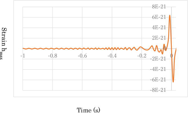
Figure 5.

Analytical calculation for the gravity wave. This figure was cited from [10]. The critical point indicates 10⁻²¹ order and the timescale is 0.1 s. The calculation agrees well with measurements and was obtained from the QEG equation solution.

3.4 Laws of electromagnetism derived from the QEG equation solution

3.4.1 Coulomb interaction and Poisson equations

Let us consider the Coulomb interaction and the satisfaction of the continuity equation regarding charge density and current density. The Poisson equations derived in the Theory section were

$$\frac{d^2\Phi }{d{r}^2}=\frac{-1}{{\epsilon }_0}\frac{c^4}{16\mathit{\pi G}}\frac{1}{v}\frac{e}{m_e{\omega }_c}\frac{1}{n}r.\left(\text{60}\right)$$

Thus, the charge density is

$$\rho =\frac{c^4}{16\mathit{\pi G}}\frac{1}{v}\frac{e}{m_e{\omega }_c}\frac{1}{n}r.$$E60-2

Eq. (60) can then be expressed as

$$\frac{d^2\Phi }{d{r}^2}=\frac{-1}{{\epsilon }_0}\frac{c^4}{16\mathit{\pi G}}\frac{e}{m_e{\omega }_c^2}\frac{1}{n}.\left(\text{62}\right)$$

For a vector potential,

$$\frac{d^2{A}_{\phi }}{d{r}^2}={\mu }_0\frac{c^4}{16\mathit{\pi G}}\frac{1}{n}\frac{e}{m_e{\omega }_c}r.\left(\text{69}\right)$$

From Eq. (62), the Poisson equation for the electrostatic potential is given by

$${\rho }_0=\frac{c^4}{16\mathit{\pi G}}\frac{e}{m_e{\omega }_c^2}\equiv {\beta }_{0}e,$$E129

where n = 1.

Generally,

$$\frac{\mathit{dQ}}{\mathit{dv}}={\beta }_{0}e,$$E130

where dv denotes the volume difference and

$$\mathit{dQ}\equiv e.$$E131

Thus,

$${\beta }_0=\frac{1}{\mathit{dv}}=\delta \left(\overrightarrow{r}\right).$$E132

Therefore, considering Eq. (62) and, as every elementary physics text states, the standard Coulomb potential forms as:

$$\Phi =\frac{e}{4\pi {\epsilon }_{o}r}.$$E133

Note that r here is the relative distance between two charged particles because of the introduction of the Dirac function with position vector r.

Next, we consider the satisfaction of the continuity equation by first considering the following elementary equation,

$$v\equiv \frac{\mathit{dr}}{\mathit{dt}}.$$E134

From Eq. (69), the current density is

$$i=\frac{-c^4}{16\mathit{\pi G}}\frac{1}{n}\frac{e}{m_e{\omega }_c}r.$$E135

Thus, the following equation is satisfied:

$$\frac{\mathit{d\rho }}{\mathit{dt}}+\frac{\mathit{di}}{\mathit{dr}}=0.$$E136

Eq. (136) can be generalized to three dimensions as

$$\frac{\partial \rho }{\partial t}+\mathit{di}\mathit{v}\overrightarrow{\iota }=0.$$E137

Considering the satisfaction of both Eqs. (133) and (137), the Poisson equation for a vector potential is automatically proved. This is because the charge density and continuity equations have been proved. The current density, i.e., the Poisson equation for a vector potential as in Eq. (69), has also been proved.

3.4.2 Newtonian equation

Let us consider the energy of quantized space time in terms of the magnetic field (or gravity field).

In the Theory section, we derived

$${\Phi }_G/2=\frac{-1}{8\pi }\frac{1}{16\mathit{\pi G}}\frac{c^2}{m_e}g\frac{1}{r}.\left(\text{78}\right)$$

Note that the 1/2 implies the symmetry of the flux direction of the magnetic field is broken, as considered in Figure 1. Using Eq. (78), we can calculate the gravity energy of a quantized space time in terms of magnetic or gravity field. If ${\Phi }_G$ has the unit [J], then parameter g has the unit $\left[J\bullet m^6\right]$. Thus, for Figure 1 and considering the flux of the central circle,

$$g\equiv 1\bullet {\lambda }_c^6\approx 1\bullet {\lambda }_0^6$$E138

and in Eq. (78)

$$r\equiv {\lambda }_c\approx {\lambda }_0.$$E139

Because we are now calculating the energy of the magnetic field quantized space time in Figure 1 (i.e., not the quantized space–times in terms of electric fields having embedded electrons, which have rest energy), the remaining energy among factor g is assumed to be the unit number one, which indirectly implies the existence of dark energy. Then, the potential is.

$${\Phi }_G=-5.8\times {10}^{-10}\mathrm{J}$$E140

which is approximately equal to U_B in Eq. (117).

Using Eq. (118),

$$M_{\tau }=1.8\mathit{GeV}/c^2.$$E141

Thus, Eq. (141) is approximately the remaining energy of a τ-particle [9] and also implies the energy of a quantized space time in terms of magnetic or gravity field. This value agrees with reported measurements and does not contradict the theory of this paper.

Note that the above Newtonian equation has a different shape from the standard Newtonian gravity equation usually taught in high school. However, although the standard Newtonian gravity equation is applied in the scale of the solar system, it is unnatural to consider that it can be applied on the quantum scale because every physics equation generally has application scales. For example, the equation ma = F is well applied in macroscopic scales but cannot be applied in scales less than an atomic one. Thus, the success of Schrodinger’s equation in application to the H atom comes not from the fact that the value of the standard Newtonian gravity equation is too small but from the fact that it is already considered inapplicable to the atomic scale.

3.4.3 Derivation of the time-dependent Maxwell’s equations

Using the solution of the QEG equation,

$$r_i^2\equiv \left(-2\right)\frac{8\mathit{\pi G}}{c^4}\frac{\frac{1}{2}ħ{\omega }_i}{{\lambda }_c^3}+{\left(c\frac{2\pi }{\omega }\right)}^2,\left(\text{30}\right)$$

we converted divisions of quantized space–times ${\lambda }_c$ and $t_c$ into standard differentials [1] to ensure the mathematical equation in the Theory section. Considering the Lorentz conservation regarding differentials, we derived the following equations:

$$\mathit{rot}\overrightarrow{H}=\frac{\partial \overrightarrow{D}}{\partial t}\left(\text{101}\right)$$

and

$$\frac{\partial \overrightarrow{B}}{\partial t}=-\mathit{rot}\overrightarrow{E}.\left(\text{116}\right)$$

Therefore, we claim that the above two equations are the same.

4. Discussion

4.1 Summary of the key points of this study

By introducing quantized space times derived from the zero-point energy, electromagnetic and gravity fields, including dark energy, are analytically well explained using the QEG equation. To this point, the only relevant concepts are zero-point energy and conservation of angular momentum of quantized space times.

4.2 Analytical solution to the QEG equation

The analytical solutions of the QEG equation resulted in various significant results. First, quantizing Einstein’s gravity equation enables us to obtain the analytical (not numerical) solution that describes every electromagnetic and gravity field uniformly. According to our previous paper [1, 2], weak and strong interactions are essentially equal to static electromagnetic fields with consideration of the zero-point energy. Thus, this paper reinforces the results of our previous paper [1, 2], which describes unified field theory in terms of particle physics while indicating that the only source of every field is the zero-point energy. Moreover, the QEG equation solutions effectively describe existing phenomena in terms of the universe.

4.3 CMB emission

The analytical solution of the QEG equation also describes CMB emission. This result implies that we are not employing the standard big-bang model. We derived CMB emission and a unique angular frequency that is a result of the QEG equation solution. The significance is that emission and absorption of CMB photons occur everywhere in our universe, and these emissions are directly related to the e-neutrino self-energy, which fluctuates in the energy level of the vacuum. Thus, CMB can be described without the standard big-bang model, and we thus claim that the measured CMB does not have the meaning of the initial time of birth of the universe.

4.4 Unified field in terms of electromagnetic and gravity fields

The analytical solution of the QEG equation also describes the unified field in terms of electromagnetic and gravity fields. This solution implies rotation of quantized space times both in terms of an electric field and a magnetic field (gravity field). The results lead to the Poisson equations regarding electrostatic, vector, and gravity potentials. These equations result in the Coulomb equation, Biot-Savart’s law, which is derived from the Poisson equation for vector potential, and the Newtonian gravity equation.

In terms of the quantized space times, induction from both electric field to magnetic field and magnetic field to electric field are derived. Thus, the time-dependent Maxwell’s equations are described. In short, the existing Einstein’s gravity equation already contains properties of both electromagnetic and gravity fields. Thus, we claim that to obtain the unified field theory, it is not necessary to expand the existing Einstein’s gravity equations, such as in five dimensions.

The most important point of this work is that all equations from electromagnetic and gravity fields come from the conservation law of angular momentum in terms of quantized space times. As mentioned in our previous paper [1, 2], weak and strong interactions are equal to electromagnetic fields and, thus, most microscopic fields and basic equations stem from the conservation law of angular momentum in terms of quantized space times. That is, only the zero-point energy is the source needed to create most fields.

Furthermore, the result of the analytical solution of the QEG equation automatically leads to the analytical derivation of gravity waves. The significance of this is that, although thus far gravity waves have only been obtained from numerical analysis of the existing Einstein’s gravity equation, we have now derived them from the pure analytical solution of the QEG equation. This comes from the fact that we succeeded in the quantization of Einstein’s gravity equation.

4.5 Three generations of leptons

Considering the basic configuration, including quantized space times in terms of both electric field and magnetic (gravity) field and the collapse of this configuration, we derived rest energies of both τ- and μ-particles that agree with measurement values. Considering that the real electron is the result of the collapse of the quantized spacetime configuration, we have now succeeded in providing the reason why leptons have three generations. The concept of quantized space times, in terms of electric, magnetic, or gravity field with zero-point energy, can be proven by comparison with measurements. In our previous paper regarding neutrinos [3], we described the three generations of neutrino, i.e., the oscillation of neutrinos and their self-energy, under the assumption that the masses of the three leptons are known in advance. However, we have now clarified all masses of the three leptons without assumption, and the most important mystery of why elementary particles have three generations was uncovered.

5. Conclusion

With the introduction of quantized space times derived from the zero-point energy and their conservation of angular momentum, i.e., the analytical solution of the QEG equation, we have created most laws and equations in terms of electromagnetic and gravity fields. Moreover, the configuration of quantized space times provides the reason why leptons have three generations.

The solution of the QEG equation also resulted in what is referred to as dark energy and the analytical derivation of gravity waves, which all agree well with reported measurements.

Conclusively, in this chapter, the gravitational wave was obtained using analytical calculations. Until now, this was only obtained using numerical or fitting methods.

With the combination of the results from our previous paper [1, 2], we have reinforced a unified field theory in terms of particle physics that indicates that concepts of zero-point energy and quantized space times describe most fields (i.e., electromagnetic field, gravity field, weak interaction, strong interaction, leptons, neutrinos, quarks, protons, neutrons, and so on). We selected the zero-point energy (i.e., the basic configuration of quantized spacetimes) as the basic source that describes almost all fields, including the masses of W and Z bosons. However, there is also the Higgs boson, which has not been described here or in our previous work. As a follow-up, it is necessary to achieve a consistent description that includes this boson.

Acknowledgments

1. We thank Enago (www.enago.jp) for their many times English language reviews.

2. We appreciate that the preprint version for this chapter can be accessed as Ref. [10].

Notation

The preprint version exists for this chapter. Please see Ref. [10]. There are some similarities as this preprint. However, these sources are from my original paper which is available online as preprint. However, in the preprint, there are a few careless errors in writing equations, and thus these have been modified in this chapter. Moreover, the logical flow in every portion of the preprint was checked and was revised in this chapter.

Additional information

This paper is not related to any competing interests such as funding, employment, and personal or financial interest. Moreover, this paper is not related to any non-financial competing interests.

References

- 1.
Ishiguri S. A unified theory of all the fields in elementary particle physics derived solely from the zero-point energy in quantized spacetime. Preprints. 2019:2019070326. DOI: 10.20944/preprints201907.0326.v1 - 2.
Ishiguri S. Studies on quark confinement in a proton on the basis of interaction potential. Preprints. 2019:2019020021. DOI: 10.20944/preprints201902.0021.v1 - 3.
Ishiguri S. Theory on neutrino self-energy and neutrino oscillation with consideration of superconducting energy gap and Fermi’s Golden rule. Preprints. 2019:2019100080 - 4.
Neronov A, Vovk I. Evidence for strong extragalactic magnetic fields from fermi observations of TeV blazars. Science. 2010; 328 :73 - 5.
Tavecchio F et al. The intergalactic magnetic field constrained by Fermi/Large Area Telescope observations of the TeV blazar 1ES 0229+200. Monthly Notices of the Royal Astronomical Society. 2010; 406 :L70 - 6.
Riess AG et al. Observational evidence from supernovae for an accelerating universe and a cosmological constant. Astronomy Journal. 1998; 116 :1009 - 7.
Kawabata T et al. Time-reversal measurement of the p-wave cross sections of the 7Be(n,α)4He reaction for the cosmological Li problem. Physical Review Letters. 2017; 118 :052701 - 8.
Ishiguri S. Analytical descriptions of high-Tc cuprates by introducing rotating holes and a new model to handle many-body interactions. Preprints. 2020:2020050105. DOI: 10.20944/preprints202005.0105.v1 - 9.
Hara Y. Elementary Particle Physics. Shokabo in Tokyo; 2003. p. 191 - 10.
Ishiguri S. Unified field theory for electromagnetic and gravity fields with the introduction of quantized space–time and zero-point energy. Preprints. 2020:2020070462. DOI: 10.20944/preprints202007.0462.v1 - 11.
Abbott BP. GW150914: The advanced LIGO detectors in the era of first discoveries. Physical Review Letters. 2016; 116 :061102 - 12.
Cutler C et al. The last three minutes: Issues in gravitational-wave measurements of coalescing compact binaries. Physical Review Letters. 1993; 70 :2984 - 13.
Ishiguri S. New attractive-force concept for Cooper pairs and theoretical evaluation of critical temperature and critical-current density in high-temperature superconductors. Results in Physics. 2013; 3 :74 - 14.
Ishiguri S. Potential of new superconductivity produced by electrostatic field and diffusion current in semiconductor. Journal of Superconductivity and Novel Magnetism. 2011; 24 (1):455-462 - 15.
Bennett CL et al. Nine-year wilkinson microwave anisotropy probe (wmap) observations: Final maps and results. The Astrophysical Journal. 2013; 208 - 16.
Dicke RH, Peebles PJE, Roll PG, Wilkinson DT. Cosmic black-body radiation. The Astrophysical Journal. 1965; 142 :414 - 17.
Maggiore M. Gravitational Waves, Volume 1: Theory and Experiments. Gravitational Waves. Oxford: Oxford University Press; 2007