Perspective Chapter: Determinants of Natural Gas Prices in the United States – A Structural VAR Approach

Abstract

This study examines the dynamic economic relationships between the fundamental variables that influence natural gas prices within the U.S. market. A structural vector auto-regressive (VAR) and Markov switching models were used to investigate the impact and stability of regime switches between the main drivers of natural gas prices. The result reveals that the U.S. gas market market is sensitive to temperature deviations in the short term. Crude oil and coal prices have long-run effects on natural gas prices, emphasizing energy-specific demand shocks. Mainly, coal prices determine about 73% of gas price variability for the sample period with three discernible regime switches.

1. Introduction

This study explores the dynamic interplay among the core determinants of natural gas pricing. The cost of natural gas holds significance for multiple stakeholders given its pivotal role in the heating and cooling industry, as well as its use in the generation of electricity. Consequently, understanding the natural gas price formation is crucial from both macroeconomic and micro-economic viewpoints. Nonetheless, the evolution of pricing is intricate due to numerous distinctive supply and demand traits that markets confront, including weather conditions, the effects of cross-commodity substitution, unexpected changes in storage, and fluctuations in business cycles.

It is difficult to disentangle the spillover effect of energy commodities due to their interconnected usage. For instance, natural gas could be used as an energy input to substitute crude oil in electricity production and heating and cooling in residential quarters. Xu Gong and Wang [1] have analyzed the volatility spillover effects among the four major commodities (i.e., crude oil, gasoline, heating oil and natural gas) in the U.S. futures market and found that spillovers have peaks and troughs during pivotal periods in history such as the U.S. shale gas discovery, the Great Financial Crisis and the oil price crash. Wang et al. [2] show that increasingly financial market factors such as investor speculation are becoming important in natural gas price formation. Notwithstanding the financialization of energy commodities, there are other fundamental factors that affect the price formation of commodities. More specifically, natural gas may have regional and international factors that drive price formation. Zhang and Ji [3] and Wang et al. [4] emphasize that natural gas markets have strong regional characteristics. As such research findings from different regions of the world such as Europe, China and the U.S. may not always be consistent. For example, Nick and Thoenes [5] find that storage conditions have a significant effect on natural gas prices following a logical economic narrative in Germany. Elsewhere, Wang et al. [2] find that storage conditions have marginal input in natural gas price movements in the U.S. The regional discrepancies may arise for several reasons. In the U.S. electricity providers who use most of the natural gas have operation mechanisms that allow them to switch between inputs (i.e., natural gas and coal). The regional price formation of natural gas prices can also be attributed to liberalization of hubs. Wang et al. [4] show that the Chinese market’s price of natural gas trades at a premium because of its link to oil indexation and not necessarily driven by market fundamentals. Specifically investigating the volatility in prices, Hailemariam and Smyth [6] report that gas prices are responsive to structural supply shocks in the U.S. citing several prominent events such as Hurricane Katrina, Global financial crisis and the discovery of shale resources. Moreover, technological and climate change polices continue to evolve the landscape of the gas market in the U.S.

In this research, five fundamental drivers of natural gas prices are identified in the U.S. gas market. The supply and demand interactions of temperature and storage deviations, short-term interest rate, coal, and crude oil prices are analyzed as variables that affect natural gas prices. We develop a structural vector auto-regressive model (VAR) and a Markov Switching process to investigate the phenomena. The models yield insights into the dynamic relationship between the variables under study. The impulse response simulations from the VAR model are consistent with economic reasoning, implying that natural gas prices react to underlying supply and demand shocks. Natural gas prices rise in reaction to abnormal temperatures, which increases heating and cooling demands in the short term. The response of gas prices to structural shocks of storage is insignificant from this study. However, the empirical results reveal that storage level depletes through withdrawals in response to extraordinary temperatures, which increases demand for heating or cooling. Coal and crude oil price shocks show long-term effects on the natural gas price formation.

A significant contribution of this research is identifying the distinct contributive effects of the different variables on natural gas prices. It is interesting to find coal prices determining about 73% of gas price variability for the sample period, unambiguously making it a systematic determinant of natural gas prices. A three-state Markov switching process between coal and gas prices has been identified with noticeable regime switches.

The discovery that the cost of coal is the main determinant of natural gas prices could question the conventional notion that crude oil is the key factor in determining gas prices. For example, Hartley and Medlock [7] and Brown and Yucel [8] argue that gas and crude oil prices are co-integrated in the short and long run. However, the stability of this cointegration dynamics is not stable over time. Wang et al. [2] and Ramberg and Parsons [9] bring to bear that the cointegration relationship between oil and gas in the U.S. market decouples over time. Particularly, Wang et al. [2] demonstrate the declining role of oil prices in natural gas pricing mechanism with time-series data between 2001 and 2018. This is due to the demise of crude oil indexation of natural gas prices. The findings of this paper is consistent with an earlier work by Nick and Thoenes [5] who find a similar strong evidence of connection between coal and natural gas prices in Germany.

In the past, the cost of crude oil has been perceived as the most influential element impacting long-term natural gas prices. A straightforward guideline, known as the 10-to-1 rule, was dominant in the 1990s. This rule proposed that the price of natural gas was one-tenth that of crude oil, as indicated by Brown and Yucel [8]. This trend of linking prices to oil has shifted in recent years, particularly in the United States, as a result of the shale gas revolution that started in 2005. With the successful application of horizontal drilling and fracking technologies, shale gas production has increased exponentially, accounting for about 79% of total gas supplies in the U.S.

The description of the data used are discussed in Section two. Section three outlines the empirical methodologies employed in previous research on the natural gas market, definition, and identification of the structural VAR model. Empirical results in the form of impulse responses and Markov switching processes are explained in Section four. A summary and conclusion are presented in Section five.

2. Data description

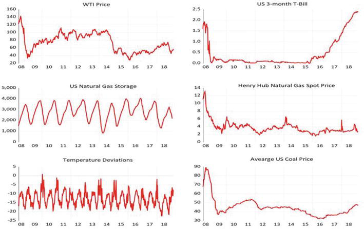
The dataset used in this research consists of 471 observations of weekly data within the period from January 2, 2010, to December 29, 2018.¹ It comprises the Henry Hub natural gas spot price, West Texas Intermediate (WTI) crude oil spot price, average U.S. spot coal price, U.S. natural gas storage, the annual yield on 3-month U.S. Treasury Bill, and the consumption-weighted temperature deviations from historical averages for the top 5 natural gas consumption states in the U.S.²Figure 1 displays all the time series of the variables and Table 1 provides a summary definition of the variables used in this study.

Figure 1.

Time series of all variables used.

Variable	Description	Unit	Source
Temperature deviations	Measured as the degrees day (D.D.) deviations from historical averages. DD = CDD + HDD. Where CDD is cooling degrees day and HDD is heating degrees day	Degrees Fahrenheit	National Weather Service (NWS)
WTI price	West Texas Intermediate spot price for U.S. crude oil	USD
Per barrel	Bloomberg
Coal price	The average spot price of U.S. coal from the five producing regions (Central Appalachian, N. Appalachian, Illinois Basin, Powder River Basin, Uinta Basin)	USD per ton	Quandl
Natural gas price	Henry Hub spot price	USD per million Btu (British thermal unit)	Bloomberg
Storage	Working gas in underground storage	Bcf (Billion cubic feet)	U.S. Energy Information Administration
Treasury bill	Three months U.S. treasury bill	Percent	Federal Reserve Bank of St. Louis

Table 1.

Summary description of variables used.

The choice of variables for this econometric analysis is comprehensive as it encompasses the diverse fundamental drivers of natural gas prices both on the demand and supply side. The variables used in this paper have been well studied and documented in the energy economics literature (see for examples [2, 10, 11, 12, 13]). Variables such as exchange rates are not applicable to the U.S. market it is a net exporter of natural gas. We do not consider the role of speculative investors to be a fundamental factor in this paper since we feel that they are more related to the financialization aspect of commodity market as a whole and not specific to natural gas. Spot prices are heavily relied upon due to their ability to capture significant short-term impacts, particularly those of interest, such as demand spikes triggered by temperature variations. Furthermore, Zhang and Ji [3] suggest that for the U.S. market hub prices can reflect the true value of natural gas. Here, the Henry Hub spot price was used because its price movement is considerably affected by the temperature conditions of the top 5 natural gas consumption states considered in this study.

The model was calibrated using weekly data to allow for the inclusion of coal price data, which is only available in weekly frequency while capturing short-term meteorological conditions. Prices of crude oil and coal are used as proxies for energy-specific demand. The inclusion of the spot price of crude oil is essential for capturing the interdependence between oil and gas in the domestic heating and cooling market. By incorporating coal prices into the model, the interaction between gas and coal in the electricity generation sector can be captured. This enables the representation of cross-commodity effects associated with fuel substitution (see, for example, [5]). Natural gas, coal, and crude oil price time series were transformed to their natural logarithms. This approach is consistent with macroeconomic literature (see, for example, [14]). The structural VAR (vector autoregressive) equation was estimated with log-level prices because the major interest is in the dynamic economic relationships between the selected variables with the natural gas market and not any possible cointegration or stationarity.

The natural gas demand in the residential heating market is susceptible to temperature. In a liberalized market, it is anticipated that storage operators will take advantage of predictable seasonal demand fluctuations. Hence, exceptional short-term weather conditions that result in a shift in demand are anticipated to be significant factors in gas price formation, rather than predictable seasonal patterns. Consequently, the degree day deviations (D.D.) from normal historical averages was equally constructed to determine gas prices. Temperature expressed in degree days is a quantitative index that reflects a demand for energy to heat or cool houses and businesses. Degree days (D.D.) is the sum of heating degree days (HDD) in the winter and cooling degree days (CDD) in the summer.³

$${\mathit{DD}}_t={\mathit{CDD}}_t+{\mathit{HDD}}_t$$E1

$${\mathit{CDD}}_t=\mathit{Max}\left(0,{\mathit{\text{Tave}}}_t-{65}^{o}F\right)$$E2

$${\mathit{HDD}}_t=\mathit{Max}\left(0,{65}^{o}F-{\mathit{\text{Tave}}}_t\right)$$E3

where ${\mathit{\text{Tave}}}_t$ is the average daily temperature of date $t$. The weather shock is defined as the deviation of D.D.s from the normal level over the period.

$$W_t=\sum _{i=1}^m\left({\mathit{DD}}_{t+i}-{\mathit{\text{DDNORM}}}_{t+i}\right)$$E4

where $m$ is the weather period, ${\mathit{DD}}_{t+i}$ is the degree days on day $t+i$, ${\mathit{\text{DDNORM}}}_{t+i}$ is the normal degree days which is the average degree days of the previous 30 years on day $t+i$. The use of deviations of the observed D.D. from their historical averages estimates the effect of unexpected weather conditions on gas prices.

In this study, storage data was included because storage operators are both on the supply-side (withdrawal phase) and demand-side (injection phase). Furthermore, instead of absolute volumes, the change in utilization rate was employed as an indicator of fluctuations in total storage capacity. The discrepancy between the average seasonal changes in utilization and the actual weekly changes was used as a proxy for the capacity of flexible storage to respond to storage shocks. The deep reasoning for this approach is to capture deviations from the seasonal storage utilization pattern. Natural gas production was not included since the U.S. has been a net exporter of LNG and crude oil since the shale gas boom in 2006. Three months treasury bills was fitted as a control variable. Treasury bills may affect natural gas prices because the short-term interest rate is a significant component of the cost of carrying inventories [15, 16].

3. Empirical methodology

There has been enormous empirical research on the natural gas market in recent years. A common thematic approach underlying these findings is the relationship between natural gas and crude oil prices rather than exploring how the natural gas market works. These approaches ignore the possibility of structural dynamics within the market. For example, [7, 8, 17, 18, 19] find movements in oil prices to influence natural gas prices. Brown and Yucel [8] analysis involved testing for a cointegrating relationship using a vector error correction model (VECM). In contrast, other studies conclude that there is a weak link in the so-called oil-gas relationship (see, for example [3, 9]).

Other complex and comprehensive frameworks have been used to explore and disentangle the supply and demand shocks driving natural gas prices using various structural or reduced-form models. Nick and Thoenes [5] analyze the German gas market using a structural VAR and find that weather, supply, storage, coal, and oil price shocks have a significant effect on natural gas price formation. Hou and Nguyen [20] employ a Markov switching structural VAR model to investigate the regime-dependent responses to its fundamental shocks. They find that the impact of oil on natural gas prices is relatively small and regime-dependent. Our attempt to use a structural VAR to model the fundamental drivers of weather, supply, interest rate, crude oil, and coal prices is a novel approach in U.S. gas market research.

3.1 Model definition

We utilized a structural vector autoregression (SVAR) methodology to model the interrelationships among key factors in the natural gas market. This approach allowed us to explicitly analyze the transmission channels that influence natural gas prices. To constrain the feedback effects of exogeneity of some of the variables used in this analysis, their coefficients was restricted to zero. The VAR model in its reduced form can be represented as:

$$y_t=\upsilon +A_1{y}_{t-1}+\dots +A_p{y}_{t-p}+{\epsilon }_t,{\epsilon }_t\sim \mathit{WN}\left(0,\mathrm{\Sigma }\right)$$E5

where $y_t={\left(y_t,\dots \dots ,y_{m,t}\right)}^{\prime }$ is a vector of $m$ endogenous variables, $p$ is the number of lags of each variable, and $\upsilon$ is an $m\times 1$ vector of intercepts.

The error terms are grouped into ${\epsilon }_t={\left({\epsilon }_t,\dots ,{\epsilon }_{m,t}\right)}^{\prime }$, such that the error term in each equation has a zero mean and is uncorrelated over time and homoskedastic. However, the error terms can be contemporaneously correlated with errors in other equations. Therefore, ${\epsilon }_t$ is a multivariate white noise process, ${\epsilon }_t\sim W.N.\left(0,\mathrm{\Sigma }\right)$, where $\mathrm{\Sigma }$ is an $m\times m$ variance-covariance matrix. The VAR model was specified with a length of six lags as identified by the Akaike Information Criterion. The SIC indicates a lag length of one; however, there is a strong autocorrelation in the error terms with one lag.

The instantaneous causality among the variables represented by ${\epsilon }_t$ in the reduced-form model does not allow for an economic interpretation of the error term. To remedy the situation, a structural model has to be identified as:

$$y_t=\left(I_m-A\right)y_t+A^{\ast }{y}_{t-1}+\dots +A^{\ast }{y}_{t-p}+{\epsilon }_t$$E6

where $I_m$ represents the identity matrix of order $m$, $A$ is an $m\times m$ matrix of instantaneous interaction among the variables and $A^{\ast }$ is equal to AA_(i) for $i=0,\dots ,p$. Additionally, ${\epsilon }_t={\left({\epsilon }_{1t},\dots ,{\epsilon }_{m,t}\right)}^{\text{'}}$ is a row vector of $m$ dimension which represents the structural errors with a variance-covariance matrix ${\mathrm{\Sigma }}_{\epsilon }$. As the instantaneous causality is captured by $A$, ${\mathrm{\Sigma }}_{\epsilon }$ is diagonal. By assigning the errors of the structural representation to a specific variable, it becomes possible to interpret them in accordance with economic theory. It enables a deeper understanding of the underlying economic relationships and their impact on the variable of interest.

3.2 Model identification

To identify the model, restrictions are placed on the instantaneous coefficient matrix $A$. The structural representation can be achieved by imposing $m\left(m+1\right)/2$ restrictions. The instantaneous restrictions imposed for identification of the structural VAR is summarized in Table 2.

	Temperature	Interest rate	Storage	Crude price	Coal price	Gas price
Degree days deviations	${}^{\ast }$	0	0	0	0	0
Change in 3-month T-bill	0	${}^{\ast }$	0	0	0	0
Storage deviation	${}^{\ast }$	${}^{\ast }$	${}^{\ast }$	${}^{\ast }$	${}^{\ast }$	${}^{\ast }$
Price of WTI	${}^{\ast }$	${}^{\ast }$	0	${}^{\ast }$	0	0
Price of coal	${}^{\ast }$	${}^{\ast }$	0	${}^{\ast }$	${}^{\ast }$	${}^{\ast }$
Natural gas price	${}^{\ast }$	${}^{\ast }$	${}^{\ast }$	${}^{\ast }$	${}^{\ast }$	${}^{\ast }$

Table 2.

Identification of the contemporaneous matrix.

Notes: Each row represents an equation in the VAR model with the independent variables ordered in columns. The ${}^{\ast }$ denotes the parameters estimated from the data and allow for instantaneous interaction between the variables, whereas 0 indicates that the parameter has been restricted to zero.

Since weather and interest rate are exogenous to the other variables in this analysis, they are ordered first within the matrix of contemporaneous interactions. Temperature deviations are expected to affect storage levels (via withdrawal from underground working gas) for cooling or heating purposes. Consequently, the instantaneous influence of temperature on storage unrestricted was ignored.

Storage of a commodity like natural gas is expected to be affected by the prevailing interest rate due to the cost of carrying inventory. In a high-interest rate environment, storage cost increases; therefore, the interaction between interest rate and storage was left intact. Gas price changes are expected to influence gas storage as storage operators primarily engage in inter-temporal price arbitrage. This economic rationale may drive the decisions and behavior of storage operators, emphasizing the significant impact of gas price fluctuations on storage dynamics. Furthermore, gas storage serves as a means to address temporary imbalances in supply caused by unexpected market conditions, including extreme weather events. It provides a mechanism to mitigate the effects of such disruptions and maintain stability in the gas market. Thus, contemporaneous impact of oil, coal, natural gas prices on storage is left unrestricted.

Enabling instantaneous interaction between crude oil, coal, gas prices, and temperature deviations is a logical approach. Extreme cold temperatures increase the demand for heating oil and can raise the price of WTI through this channel. The price of coal may be affected by oil and gas prices since coal serves as a substitute for electricity production. Therefore, the contemporaneous interaction between coal, gas, oil prices, and temperature are unrestricted.

The effect of interest rate across all three commodity prices (i.e., crude oil, coal, and natural gas) is unrestricted as it may have a significant explanatory power on the price variability. The overshooting model of Dornbusch hypothesizes that monetary changes have real short-run effects on commodity prices [21]. Whenever markets adjust in response to monetary changes, those sectors of the economy that are free to move (i.e., commodities and financial assets) must bear the burden of the sluggishness of the sticky sectors (i.e., manufacturing and services).

In this research, the focus is primarily on the price of natural gas as the main variable of interest. Therefore, no restrictions are imposed on that variable in the equation. This approach allows for a comprehensive analysis of the immediate impacts of all variables included in the model on natural gas prices. By considering all variables, we can understand the factors influencing natural gas prices.

4. Empirical results

4.1 Impulse response function

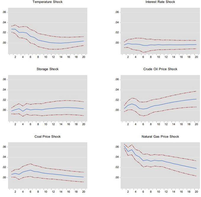
The application of the VAR model concerns the evaluation of the impact of structural shocks, which can be done using the moving average (M.A.) representation. Figure 2 presents the estimated impulse response functions for the natural gas price.

Figure 2.

Responses of natural gas prices to shock from the other variables. Notes: response is to Cholesky one s.d. innovations 2 s.e.

The response of gas prices to changes in temperature, as observed in the impulse analysis, aligns with economic narrative. Extreme temperature has an immediate and substantial impact on the price of natural gas through demand for heating or cooling in residential and business buildings. The effect is significant and declines over time but can last for as long as ten weeks, which indicates that temperature shocks have a short-term impact on natural gas prices. Short-term interest rate innovation has no significant effect on gas prices and crude oil and coal prices, which is contrary to the observed a priori assumption.

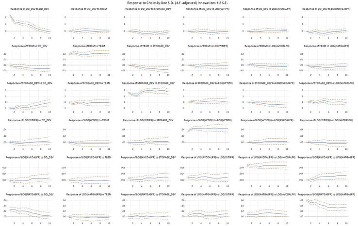
Innovations from storage do not also affect gas price movement. This finding is consistent with the results of another empirical research by Wang et al. [2], who find that the influence of storage on natural gas prices proves to be marginal in the U.S. market. Although this research focuses on the determinants of natural gas price variability, it is worth discussing the structural response of storage to all variables, as shown in Figure 3. The impulse response function reveals that extraordinary temperatures lead to storage withdrawals. This phenomenon is caused by the demand for temperature-sensitive natural gas in the heating and cooling of residential and commercial facilities. Nonetheless, the response of storage flows to natural gas price shocks is insignificant, and it may be inconsistent with economic expectations. This is because an increase in natural gas prices should incentivize storage holders to withdrawal from their inventory. This economic narrative may not be the case for U.S. market. We reason that the effect of the rise in natural gas prices in response to storage withdrawal may be muted by cross-commodity effects. Storage withdrawals occur in response to shocks in coal prices as shown in Appendix A. It could be explained by the cross-commodity relationship emphasized earlier. An increase in coal prices implies high demand; therefore, electricity producers who can switch their input move to natural gas, which affects storage levels through withdrawals. Since operators are switching from a higher price (coal) to a lower priced input (natural gas); the net change in storage may not necessarily lead to a significant price movement in natural gas. Consequently, innovations in storage leads to natural gas price stability.

Figure 3.

Impulse response functions for all variables.

Coal prices only affect natural gas prices with a delay, but its effect is substantial and remains stable over time and gradually declines. The strong inter-dependency between coal and natural gas can be attributed to the energy mix of the U.S. electricity generation industry. According to the U.S. Energy Information Administration (EIA), about 35.1% and 27.4% of total electricity generation output were from coal and natural gas, respectively in 2018. This brings about fuel competition among energy producers, which may induce a positive cross-price elasticity of these two commodities. Consequently, a rise in the price of coal implies an increase in the demand for natural gas and, therefore a resulting price increase.

The derived structural response of natural gas prices to crude oil and coal prices reveals significant inter-dependencies among energy commodities. The price of gas responds positively to innovations in both oil and coal prices. However, the pattern with which oil and coal influence gas prices is fundamentally different. Oil price shocks impact natural gas prices instantly, causing the cyclical price movement in natural gas in the short-term, but later establish a long-run relationship after that. This long-run relationship between natural gas and oil prices is plausible as there exists a physical link in their direct substitution relation in the residential heating sector.

4.2 Forecast error variance decomposition

After identifying the structural dynamics in the natural gas market, it is appropriate to investigate the fundamental influences of each variable on natural gas price movement. To this end a forecast error variance decomposition was performed using the results of the estimated structural VAR model. The variance decomposition splits the forecast error variance of each endogenous variable, at different forecast horizons, into the components due to each of the shocks. This provides information on their relative importance. The contributions of innovations in variables calculated through the moving average representation of the VAR model are presented in Table 3.

Period	Temperature	Interest rate	Storage	Crude oil price	Coal price	Natural gas price
1	0.00	0.37	0.02	16.88	72.60	10.13
2	0.00	0.18	0.02	16.99	72.79	10.03
4	0.00	0.14	0.02	17.04	72.84	9.97
12	0.00	0.32	0.01	17.00	72.83	9.84
26	0.00	0.37	0.01	17.19	72.68	9.75
52	0.00	0.40	0.01	17.37	72.50	9.72

Table 3.

Forecast error variance decomposition for natural gas price.

Notes: values are expressed in percentages.

Temperature and storage deviations unexpectedly have no explanatory power on the price formulation of natural gas. However, the forecast errors of gas prices can be explained more precisely by developments related to coal and oil markets. Coal price variations have the most impact on natural gas price variability, with maximum explanatory power in short-term horizons (4–12 weeks). Long-term natural gas price development (up to 52 weeks) is heavily affected by variations in oil prices. Coal and crude oil prices account for about 90% of the gas price variance with a forecast horizon of half a year.

4.3 Markov switching

Having identified coal prices to have the most explanatory power on natural gas price development, a Markov process was ran to ascertain gas price regime changes as explained by coal price variability. Coal prices are the first-differenced to obtain stationarity, while natural gas price series are stationary at the level.⁴ A three-state Markov switching process was identified for the interaction between natural gas and coal prices, as presented in Table 4.

Variable	Coefficient	Std. error	z-Statistic	Probability
Regime 1
C	2.72055	0.03006	90.50647	0.00000
D(COALPR)	0.20023	0.06242	3.20756	0.00130
Regime 2
C	3.85925	0.04661	82.80654	0.00000
D(COALPR)	0.20015	0.10493	1.90754	0.05650
Regime 3
C	4.96656	0.10550	47.07560	0.00000
D(COALPR)	0.09762	0.18518	0.52716	0.59810
Common
LOG(SIGMA)	−0.90061	0.03500	−25.73061	0.00000

Table 4.

Three state Markov switching regression for gas and coal price interactions.

Notes: Dependent variable is the natural gas price.

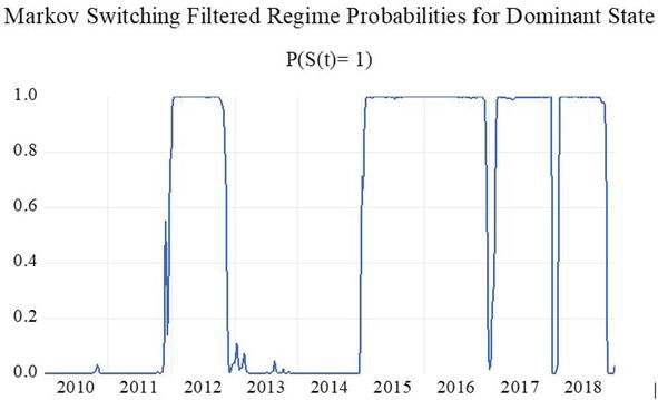
As shown in Table 4, Regime 1 shows a robust positive co-movement between gas and coal prices. Regime 2 (with a relatively moderate co-movement) does show a discernable switch from Regime 1 as observed in the coefficients. Regime 3, however, shows a weak co-movement. Explicitly, Regime 1 dominates the Markov process with a constantly expected duration of 56 weeks which is longer than the 24 weeks duration for Regime 2. The probability of remaining in that regime on any given day of 0.982 is the highest.

The results mean that when there is a strong co-movement between natural gas and coal prices, one can expect it to last for a long as a year which is a high probability. Displayed in Figure 4 are the filtered switching probabilities for the Dominant Regime 1.

Figure 4.

Markov switching probabilities for Regime 1.

5. Conclusion

Thus far, this paper has investigated the dynamic interaction between the fundamental variables within the U.S. natural gas market. The analysis is conducted with structural VAR and Markov switching models. This approach allows us to disentangle the effects of different fundamental influences on natural gas prices. The empirical results reveal that abnormal temperatures affect natural gas prices in the short term. However, the price development of natural gas is closely tied to crude oil and coal prices in the long term, indicating the high importance of cross-commodity effects.

The specific contribution of the main fundamental drivers of gas price formation within the period under study was explicitly analyzed. Results from this study revealed that coal prices account for about 73% of the price variability of natural gas prices with a persistently strong regime switch. The results of this research are relevant to storage operators, electricity producers, and speculative investors in strategy formation and operations. As the results of this research are compelling, it cannot be generalized as natural gas prices are mainly determined by regional supply, demand, and temperature variations (see, for example, [3]). The approach provides an innovative framework for further research on more specific economic mechanisms within the U.S. gas market. Additionally, this model can be used to study other regions within the U.S. The current application is still restricted by the limited data on certain variables used in this research. A future attempt will be made to generalize the findings for the entire U.S. gas market when more data become available.

This chapter was initially published as a preprint: Nkwantabisa D. Determinants of Natural Gas Prices in the United States—A Structural VAR Approach [Internet]. SSRN Electronic Journal. Elsevier BV; 2021. Available from: http://dx.doi.org/10.2139/ssrn.3905560

JEL classifications

C32, E32, G13, Q40