Recent Advances in Machine Learning Methodologies for LIBS Quantitative Analysis

Abstract

The mapping between LIBS spectral data to the quantitative results can become highly complicated and nonlinear due to experimental conditions, sample surface state, matrix effect, self-absorption, etc. Therefore, the accurate quantitative analysis is the longstanding dream of the LIBS community. The advantages of machine learning in dealing with high-dimensional and nonlinear problems have made it a cutting-edge hot topic in quantitative LIBS in recent years. This chapter introduces the current bottlenecks in quantitative LIBS, sorts out the data processing methods, and reviews the research status and progress of conventional machine learning methods such as PLS, SVM, LSSVM, Lasso, and artificial neural network-based methods. By comparing the results of different methods, the perspective of future developments on learning-based methods is discussed. This chapter aims to review the applications of the combination of quantitative LIBS and machine learning methods and demonstrate the performance of different machine learning methods based on experimental results.

1. Introduction

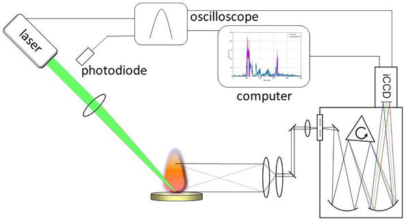
Laser-induced breakdown spectroscopy (LIBS) is a noninvasive spectroscopy technique based on the emission from the excitation of atoms in materials, and it is widely applied for elemental compositional analysis. The sketch of the LIBS is illustrated in Figure 1. The spectra and images of the plasma plume produced by the pulsed laser ablation onto the sample surface are collected by the spectral-resolved measurement devices. The electrons and ions/atoms ejected from the sample can represent the quantitative characteristics (e.g. elements, concentrations, etc.) of the target, and LIBS offers a spectrometric method to obtain the information of samples.

Figure 1.

The sketch of the LIBS method.

The quantitative results can be obtained by analyzing the spectrum emitted from the plasma produced by a pulsed laser irradiation. Due to its capabilities of standoff and online measurements, portability, quasi nondestructive detection, etc., LIBS has widely used in the fields of environmental monitoring, space missions, industrial monitoring, and isotope analysis. Several excellent existing works have reviewed LIBS applications [1, 2, 3, 4], mainly focusing on specific areas or techniques such as diagnosis of the plasma-facing wall of confinement fusion devices [5, 6, 7], industrial applications [8, 9, 10] and data analysis [11], nanoparticles in LIBS [12, 13], underwater applications [14], aerosol analysis [15], and the study of uranium-containing compounds [16].

Since the physics and chemical mechanism involving complicated processes, including laser-sample target, laser-plasma, and plasma-sample interactions, the emission spectra are sensitive to laser parameters, ambient gas pressure, target characteristics (e.g. heat capacity, thermal conductivity, surface roughness, wavelength-dependent absorptivity, etc.). Their temporal and spatial evolving [17, 18] lead to complex nonlinear mapping from spectral data to quantitative results, thus, the accuracy and real-time performance of quantitative LIBS needs further improvements. In recent years, the rapid developments of machine learning and deep learning methods have received extensive attention from LIBS community due to their brilliant capability for solving nonlinear problems. Chen et al. [19] summarized machine learning methods in the LIBS analysis of geological applications. Li et al. [3] reviewed artificial neural networks (ANN) methods in geology, biology, and industrial applications, demonstrating the potential of ANN-based LIBS for material identification/classification and quantitative analysis. Zhang et al. [11] focused on evaluating the performance of conventional machine learning methods, such as principal component analysis (PCA) and support vector machines (SVM), on LIBS classification and regression. Huang et al. [20] provided a review of machine learning-based LIBS in soil analysis tasks.

These works concluded the comprehensive application of machine learning methods in LIBS classification and regression tasks; however, quantitative analysis, especially accurate quantitation, is still the vital barrier for LIBS toward real-world practicality. Since different types of data processing methods and machine learning methods have their own strength and inadequacy, it is of great importance to analyze and optimize one or hybrid appropriate methods according to application scenes and tasks. While at present, few reviews specifically focus on the comparative analysis and outlook of learning-based methods for quantitative LIBS. Following prior excellent reviews, this chapter emphasizes on machine learning techniques in quantitative analysis and summarizes the existing methods and advances in combination with the latest artificial intelligence (AI) results and development trends. Based on the latest experimental results, we propose a perspective on the future development of learning-based quantitative LIBS from the viewpoint of AI-driven LIBS research.

2. LIBS data preprocessing methods

LIBS system usually includes pulsed lasers, laser focusing optics, spectral collection optics, spectrometers, spectral calculation, and interpretation devices. Nanosecond lasers are the most common-utilized LIBS light sources in laboratory and industrial scenarios due to its advantages of small size and weight, low cost, and portability. In recent decades, with the development of ultrafast laser technology, femtosecond lasers have also been applied to LIBS analysis with benefit of their characteristics, such as smaller ablation volume and cold ablation effect [21].

Although the LIBS hardware system seems to be relatively simple at first glance, the laser characteristics (e.g., wavelength, pulse width, energy), focusing characteristics (e.g., spot size, ablation rate, incident angle), target characteristics (surface roughness, absorption rate, thermal conductivity, etc.), and ambient environment characteristics (e.g., background gases and their pressures) during the process [17, 22, 23, 24, 25, 26] significantly affect the plasma emission spectra, reducing the accuracy elements concentration calculations by analyzing spectra emitted from laser-induced plasma. Despite its strength of online measurements, LIBS with conventional quantitative methods has a lower limit of detection (LOD) in comparison to those offline chemometric techniques. For trace element detection in most solids, the LIBS LOD is often in the range from 1 to 100 ppm [27], which barely meets the needs of several element trace tasks.

In order to enhance the reproducibility of LIBS spectral signals and improve the signal-to-noise ratio, spatial confinement [28], electric-field-assisted [29], magnetic-field-assisted [30], polarization enhancement [31], nanoparticle enhancement [32], and optical capture enhancement [12] have been proposed in the current study to establish stable experimental acquisition conditions in order to improve the quality of raw data. For the acquired spectral data, data preprocessing is one of the key steps for quantitative analysis of LIBS, which can effectively improve the accuracy and reproducibility of the results. Existing spectral data preprocessing methods can be classified into four categories: accumulation and averaging, data filtering, normalization and standardization, and self-absorption calibration.

2.1 Accumulation and averaging

Accumulating and averaging measured multiple spectra is effective in reducing noise and improving repeatability and signal-to-noise ratio (SNR). Theoretically, accumulating multiple spectra can improve the spectral SNR while avoiding spectral intensity saturation, and the higher the number of accumulations, the more beneficial it is to the quantitative results. However, according to the principle of statistics, if the noise affecting spectral repeatability obeys a normally distributed random noise with expectation m and standard deviation s, the expectation of the average intensity and standard deviation of the noise of the accumulated n spectral measurements are also m and s. Therefore, the larger the number of accumulations is, the smaller impact of further increase in the number of accumulations on the improvement of signal repeatability, that is. the marginal utility is decreasing.

2.2 Data filtering

Data filtering methods mainly include smoothing, mean filtering, Kalman filtering, Wiener filtering, adaptive filtering, and wavelet transform. These methods can theoretically divide the spectra into “signal” and “noise,” and then remove the “noise” part from the spectra to improve the SNR and enhance the reproducibility of the LIBS plasma and its spectra, hence the reproducibility of the LIBS plasma and its spectra is enhanced. However, it is very difficult to define “signal” and “noise” in real scenarios. For example, in steel samples, the characteristic spectral signals of trace elements, such as sulfur and phosphorus, which are usually in the order of 0.01% or less, can be easily ignored and regarded as the “noise” signal due to the insufficient SNR. Therefore, before applying filtering methods to spectral data, it is important to consider their physical background and their impact on the raw LIBS data. It is often possible to optimize the filtering method and determine the filtering parameters based on the physical mechanism of quantitative analysis. For example, moving averages and the resulting moving convolutions that can be adapted to machine learning methods are more typical spectral smoothing methods. The method can be applied to the spectra of each sample, thus reducing errors due to instrumental and environmental noise. It is important to note that the choice of the sliding window width is one of the most important parameters. If the moving window is too narrow, the smoothing effect will be limited, while if the moving window is too wide, the resolution of the spectrum will be compromised, resulting in a poor quantitative analysis.

2.3 Normalization and standardization

Spectral normalization, also known as spectral standardization, is a commonly used method to reduce signal uncertainty and improve signal concentration correlation. Normalization methods include background normalization, spectral integral normalization, standard normal variable normalization, internal standard normalization, and external standard normalization [33]. Usually, normalizing the background can effectively improve the data quality, but some of the findings also give contrast results [34].

Spectral integral method divides the spectrum intensity by the integral intensity of the whole spectrum to obtain the normalized spectrum [35]. Standard normal variational method refers to the intensity calibration to the standard normal distribution [36]. Internal standard method involves selecting the reference spectral lines in the vicinity of the interested spectral lines to calculate the relative intensities [37], and external normalization uses spectral lines from the known elemental concentration to calibrate the spectral lines of unknown elements.

Several studies on LIBS normalization are listed in Table 1. Some prior research hypothesized that normalization is expected to yield better experimental results but did not verify it by comparing experiments.

Normalization method	Norm vs. non-norm comparison	Metric parameters	Reference
internal normalization	Yes	RMSECV, LOD	Thomas et al. [38]
internal normalization	Yes	RMSEC, R^2	Andrade et al. [39]
background normalization	No	R^2, LOD	Dell’Aglio et al. [34]
spectral integral	No	RMSE, R^2	Payre et al. [40]
spectral integral	Yes	RMSECV, R^2	Takahashi et al. [41]
standard normal	Yes	R^2, LOD	Syvilay et al. [36]

Table 1.

Several existing normalization methods, where RMSECV is root mean square error of cross-validation, RMSEC is root mean square error of cross-validation, RMSE is root mean square error, and LOD is the limit of detection.

From the table, the R² is often used as an evaluation parameter, complemented by other metric parameters such as root mean square error (RMSE), root mean square error of the validation set (RMSEC), root mean square error of the cross-validation (RMSECV), and the limit of detection (LOD), which allow evaluation of the superiority from different perspective.

In addition, some studies have used other parameters from LIBS experiments as normalization references. For example, a normalization method based on plasma parameters is proposed and applied to archeological samples [42]. The total number density, temperature, and electron number density can also be used to normalize the measured spectra under different conditions in order to compensate for fluctuations in the spectral signals due to variations in the nature of the plasma [43]. A method based on the ideal sample normalization is proposed by [44]. The method assumes that the plasma temperature (T), electron number density (N_e), and atomic number density (N_s) of the measured element are at standard values in the ideal state, and each actual measured signal can be regarded as the ideal state value plus the deviation caused by the variation of T, N_e, and N_s. By converting each measured spectrum to a spectrum at the standard state, the measurement uncertainty can be reduced. Similarly, researchers have used the current of the LIBS plasma, total emission intensity, plasma images, the Euclidean norm, the maximum and minimum intensity values of each individual spectrum [45, 46, 47], and other reference signals to calibrate spectral raw data [48].

However, for quantitative analysis, the plasma does not always satisfy the local thermodynamic equilibrium (LTE). In addition, the elements with low concentration in the target yield a small intensity of the spectral lines, so the SNR is not sufficient to derive accurate quantitative results. Thus, the use of calibration methods in practical applications needs careful assessment based on the actual state of the LIBS plasma. In conclusion, although normalization can reduce the fluctuation and error of the signal under certain circumstances, the normalization method that lacks mechanism support can also lead to a worse quantitative accuracy than the non-normalized case [34]. Therefore, the selection of normalization methods should consider availability of prior knowledge, suitable reference lines, and reliable mechanistic models.

2.4 self-absorption calibration

The spectrum of spontaneous radiation in the central region of the plasma undergoes self-absorption as it passes through the region occupied by the plasma. In the measurement of relative concentration of trace elements to iron in steel samples by using the remote LIBS technique [49], nonlinear effects are still obvious due to the self-absorption even after the internal normalization. Experiments [50] have shown that even if no significant attenuation in the line shape, the self-absorption effect still presents and affects the accuracy of the quantitative results. Theoretical models for optically thick plasmas are commonly used in studies to calibrate self-absorption via the curve of growth (COG). The COG method is firstly applied to the Cr peak and analyzed the properties of the laser-induced plasma, such as temperature. The mode [51] l demonstrated the difference in the relationship between peak intensity and concentration over a wide range of concentrations. The line absorption model [52] is also used to calculate theoretical intensities from the significant self-absorbing Cu lines, demonstrating that their method is effective for generating highly linear calibration curves of the Cu/Si intensity ratio as a function of Cu concentration. Lazic et al. [53] calculated optically thick plasma self-absorption of different elemental spectral lines and showed that self-absorption can lead to relative errors of up to 20% in quantitative LIBS analysis.

The temporal–spatial evolution of LIBS plasma is complicated [25], so the self-absorption study is important to understand the mechanism of plasma emission spectra in LIBS. Existing studies have proposed many methods to reduce matrix effects and correct for self-absorption to improve the accuracy of calibration quantitative analysis. However, the effectiveness of these methods still depends on the samples and experimental conditions used. For example, for the quantitative analysis of samples with complex compositions, such as steel, rock, and soil, the nonlinear effects caused by matrix effects and self-absorption effects are still the bottleneck, which limits the high-precision quantitative analysis of LIBS.

3. Conventional machine learning methods for LIBS

3.1 Partial least squares (PLS)

Partial least squares (PLS) regression is a statistical-based machine learning method that obtains a linear regression model by projecting the prediction and observable variables onto a new space and then determining maximum variance hyperplane between the function and the independent variables. PLS has been widely used in the quantitative LIBS, especially in the quantitative analysis of samples containing multiple elements, for example, the prediction of chemical composition of rock samples [54]. The serial partial least squares (S-PLS) and multiblock partial least squares (MB-PLS) [55] are used in quantitative analysis. The hybrid method [56] of PLS and wavelet transform is proposed to measure the C content in 24 bituminous coal samples. Since the output of the PLS method is not limited to elemental concentrations, it has also been applied to other quantitative analyses. For example, C element, ash, and volatile components in 58 coal samples are determined by a combined model [57] of principal component analysis and partial least squares. The isotopic ratio of U235/U238 is outputted with relative error of 0.1–8% [58], whose accuracy can meet the demand of in situ detection for industrial production.

The PLS method is not only used for the detection of samples in atmospheric environment but is also applied to underwater LIBS measurements. Large fluctuations occurred in the signal of LIBS in water by PLS and improved the accuracy of the quantitative analysis, which resulted in a reduction of the RMSECV by 30% [59]. In addition, the PLS method has been applied to the in situ analysis of Martian rocks by ChemCam, a LIBS device on board Curiosity [60, 61]. Experimental results in laboratory and practical environments [62, 63, 64, 65] show that PLS quantitative analysis achieves better results with a 9% reduction in RMSEP compared to other multiple regression methods, such as elastic net, least absolute contraction, and selection operators, support vector regression and k-nearest neighbor regression [66, 67].

Since PLS has theoretical advantages in dealing with multivariate regression problems, the PLS method outputs more accurate results under the circumstance that more variables than observed condition numbers in the prediction matrix, or when there is multicollinearity among the data. It is important to note that PLS relies on statistical correlation or curve fitting, ignoring the physical knowledge of the LIBS measurements, which may lead to excessive noise and ultimately undermine the accuracy of quantitative measurements if the samples are out of the range of calibration sample set. Therefore, PLS should be used in combination with methods that incorporate physical mechanisms, such as principal component analysis and wavelet transform, to obtain better analytical results.

3.2 Support vector machine (SVM)

SVM is a machine learning method based on the principle of structure minimization, which is suitable for multivariate regression problems and has strong adaptability to high-dimensional, complex, and nonlinear data. SVM is widely used in quantitative LIBS, and fusion of principal component analysis (PCA), which reduces the dimensionality of the data, with SVM is a common approach in LIBS.

The combination of PCA and SVM can analyze ash, volatile matter content, and calorific value in 550 kinds of coal samples [68] and can establish calibration model for 35 kinds of coal samples after spectral normalization by Lorentzian and linear functions [69]. Experiments [70] reveal that SVM method could effectively reduce the model complexity and obtain more accurate results of silicon, magnesium, calcium, iron, and aluminum elemental concentrations. However, SVM is not robust to noise, it needs to consume a lot of computational resources and the speed is slow when regression analysis is performed on spectral data embedded with different kinds of noise in the real scene. A combination [71] of particle swarm optimization (PSO) algorithm with the SVM algorithm is proposed to measure the concentration of heavy metal chromium Cr in pork, and both R² and RMSE are reduced compared to the traditional SVM method. Compared with the artificial neural network-based quantitative analysis presented in the following section, the SVM method has the advantages of simple parameter control and high interpretability.

Least squares support vector machine (LSSVM) is an improvement of SVM. In LSSVM, the least squares method is used to solve the problem of classification or regression instead of the convex optimization problem in SVM. Thus, LSSVM has a simpler solution process, faster computation and can handle high-dimensional sparse data. In addition, LSSVM can optimize the performance of the model by adjusting the regularization parameters and the parameters of the kernel function. Results of LIBS quantitative analysis on Al-Cu-Mg-Fe-Ni alloy samples [72] show better performance of LSSVM method than PLS regression from the perspective of prediction accuracy, model robustness, computational time, and generalization ability. Prior work [73] also quantitatively analyzed atmospheric deposition of four metallic elements (Pb, Cu, Zn, and Al) by fusion of random forest with the LSSVM method. The predictive performance of different models was evaluated via metric parameters such as accuracy, sensitivity, precision, and specificity, and the LSSVM model showed superiority in pollution sources LIBS experiments.

3.3 Least absolute shrinkage and selection operator (LASSO)

In statistics and machine learning, the least absolute shrinkage and selection operator (LASSO) is an often-used regularization-based regression analysis method. Its basic principle is to constrain the complexity of a linear model by applying an L1 regularization term to the model to improve the predictive accuracy and interpretability of the generated statistical model. The Lasso regression can be generally expressed as

$$\hat{\beta }=\underset{\beta }{\text{argmin}}\left\{{\displaystyle \sum _{i=1}^N{\left(y_i-{\beta }_0-{\displaystyle \sum _{j=1}^P{x}_{ij}{\beta }_j}\right)}^2+\alpha \sum _{j=1}^P{\Vert {\beta }_j\Vert }_1}\right\}$$E1

The advantage of using these linear methods is to prevent overfitting due to the application of penalty terms. The method can be used even if the number of predictions in the dataset is greater than the number of observations. It is also computationally efficient in terms of learning and prediction. The Lasso algorithm can be used to optimize the feature parameter selection in machine learning by ranking the correlation between the different elemental concentration in the sample and the spectral intensity. The larger the absolute value of the Lasso coefficient β indicates the higher correlation between the intensity and the concentration of the element. Therefore, it is very suitable for quantitative LIBS for those samples with many elemental species and large differences in concentration. For example, Boucher et al. [67] used the LASSO regression method to quantitatively analyze the principal components of rocks. Zhang et al. [74] quantitatively analyzed the C element in steel samples, and the relative error was reduced to 13.6%.

4. Artificial neural network (ANN)

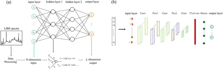
Neural network is a powerful and effective analytical method for describing the mapping relationship between the input parameters I, $I\in {\mathbb{I}}^m$ (m-dimensional feature space $\mathbb{I}$) and the output result O, $O\in {\mathbb{O}}^n$ (n-dimensional result space $\mathbb{O}$). The method can model complicated systems, including causal and logical reasoning based on knowledge of physics, chemistry, etc., and stochastic processes such as noise by using datasets to train artificial neural network (ANN) and finally accomplish regression analysis task. Specifically for LIBS quantitative analysis, neural networks can construct models to learn the mapping relationship between input parameters such as spectral intensity, spectral line shape, spectral center wavelength, plasma characteristic parameters, experimental condition parameters and output parameters such as the concentration of each element in the sample, containing spectroscopic processes based on physicochemical mechanisms, matrix effects, self-absorption, background noise, random noise, signal fluctuations, and any processes that interfere with the linear/nonlinear relationship between input–output parameters. With sufficient data and appropriate training, neural networks can theoretically achieve high-precision quantitative analysis for complex LIBS processes (Figure 2).

Figure 2.

The common-used ANN structures. (a) Sketch of BPNN, (b) sketch of CNN.

4.1 Back-propagation neural network (BPNN)

BPNN is a kind of ANN based on error back-propagation algorithm. BPNN can adaptively learn complex nonlinear relationships, the training speed is fast, and the effect is more prominent when the amount of data is not large. As a supervised learning method, BPNN needs some known samples for training and then uses some unknown samples to test the performance of the training network. For the quantitative analysis of elemental concentration, all samples are usually divided into training, validation, and test samples, and accordingly, the whole LIBS spectral dataset is divided into training, validation, and test sets. The initial weights and bias values of the original BPNN are randomly assigned. When BPNN training is performed, the spectra of the training samples are input into the network along with their concentration truth values. The output concentration values predicted by the BPNN are then compared with the measured values and the total error between them is calculated, and this is iterated for many rounds until the total error converges to the desired value or the number of iterations reaches the pre-set upper limit, thus obtaining a set of final weights and bias values that constitute the convergence of the trained network to the appropriate range. Finally, the predictive ability of the evaluated model is examined by validation and test sets. The trained network predicts and calculates the elemental content in the sample, and its accuracy can be assessed by the difference between the actual and predicted values.

As mentioned above, the problem of the reproducibility of LIBS raw data spectra and the fluctuation of experimental parameters, such as laser energy and plasma temperature, can seriously affect the accuracy of the calculation of the elemental content of the samples. Researchers have solved the problem by building BPNN networks containing experimental parameters. For example, Wang et al. [75] proposed a method for quantitative analysis of LIBS based on key parameter monitoring and back-propagation neural network, called KPBP [76], which used the BPNN algorithm to fit the spectral intensities, and standardized the spectral segments containing the characteristic lines using KPBP. In the study, KPBP experiments were first carried out on the spectra of monolithic samples such as pure aluminum, monocrystalline silicon, and pure zinc in order to optimize the KPBP model. The results show a significant reduction in the RSD of the quantitative results obtained by KPBP compared to the conventional machine learning method and the BPNN method.

4.2 Multilayer perceptron (MLP)

MLP is a common feedforward neural network. It consists of multiple neurons connected through multiple layers. Its basic principle is to pass the output obtained by weighted summing the inputs of each node to the nodes in the next layer through the activation function, and at the same time, to perform nonlinear transformations and dimensionality reduction on the data, to better characterize the structure of the data, and to deal with the complex nonlinear problems. Compared with BPNN in quantitative LIBS, MLP has higher model complexity and fitting ability. However, MLP also suffers from the overfitting problem and requires a suitable regularization method to constrain the learning process of the neural network. Bhardwaj et al. [77] developed a semi-supervised learning method based on an adaptive MLP algorithm for long-range portable LIBS systems. The method is lightweight, low computational, and power cost, and the model training and prediction can be deployed on commercial cell phones with accuracy of 89.3% for quantitative analysis. Effects from experimental parameters and physical and mechanical properties of samples are studied [78] by designing the network inputs, including the laser single-pulse energy, the iCCD time delay, ionization energy of the measured element, the central wavelength of the corresponding spectral line, the concentration of individual elements, the reflectivity of the sample, the latent heat of vaporization, the specific heat, and the boiling point, in the MLP network model, which is used to obtain the optimal SNR of the LIBS spectra. The results show that the experimental parameters can be optimized efficiently using the MLP method, so it is possible to select the experimental parameter corresponding to the best SNR value as the optimization parameter for LIBS measurements and improves the performance of LIBS measurements. Both BPNN and MLP are shallow neural network algorithms, and they are highly adaptive, flexible, and predictive accurate. When choosing a specific algorithm, it is necessary to consider the data volume, sample characteristics, prediction accuracy, and other factors and choose a suitable neural network structure according to the actual situation.

4.3 Convolutional neural network (CNN)

CNN is a deep neural network method commonly used in quantitative LIBS analysis. Compared with the BPNN and MLP networks, the modules of convolution and pooling in the CNN framework achieve better performance in processing nonlinear LIBS spectral data. The basic principle of CNN in quantitative LIBS is to extract the internal correlation of the neighboring data points through the convolution operation to learn the deeper features in the LIBS spectrum.

Due to the rapid development of CNN models, CNN methods have been a hot research topic in quantitative LIBS research in recent years. Yang [79] and Li [80] et al. studied LIBS spectra collected during the preflight test of the Mars mission based on the Mars Surface Composition Detector (MarSCoDe) on Tianwen 1 Mars Rover, achieved high-precision quantitative LIBS by using a CNN model with five convolutional layers and two pooling layers. Castorena et al. [81] proposed a CNN network dedicated to spectral processing, which can simultaneously realize the preprocessing and quantitative measurement of LIBS spectral signals, and the experimental results demonstrated that this method was significantly better than the existing method used by the U.S. Mars rover Curiosity. Davari et al. [82] fused the Lasso model with a one-dimensional CNN method to analyze LIBS spectra of single-crystal silicon and measured the oxygen-related impurities in the samples with LOD as low as 0–16 ppm. Cui et al. [83] proposed a migration-learning multitask regularized CNN model for quantitative analysis of coal samples on a dataset with small sample size. Compared with PLS, SVM regression, and ordinary CNN networks, the RMSE of this method was reduced by 19.9%, 5.9%, and 7.7%, respectively. Choi et al. [84] used LIBS to monitor laser cleaning of painted stainless steel and proposed a deep learning method based on CNN for quantitatively analyzing whether the base elemental material appeared in LIBS spectra and achieved satisfied results in terms of real time and accuracy. Eynde et al. [85] used the CNN-architected GHOSTNET network for trace elements such as Fe, Cu, Mn, Mg, and Zn, which are found in very low levels in fertilizers, and compared it with the BPNN method. The results show that the average RMSE of the deep learning method does not exceed up to 0.01%. In addition, the method is lightweight and real time with processing time only 10 ms, which plays an important role for the practical application of LIBS technology in metal sorting and other fields.

In conclusion, CNN can mine the intrinsic features and distribution of data and is a more accurate quantitative LIBS method. In practical applications, the appropriate network structure and training strategy can be selected according to the data characteristics and the constraints of computational resources to improve the accuracy and robustness of quantitative analysis.

In addition to the above commonly used neural networks, there are other deep learning methods that have been applied to LIBS quantitative analysis. For example, Wei et al. [86] used the wavelet neural network (WNN) to quantitatively analyze the main components in coal ash, and the results showed that WNN still has high accuracy in online detection. Rezaei et al. [87] used recurrent neural network (RNN) to compare the accuracy of quantitative analysis of aluminum alloy with other methods, such as SVM regression and MLP, and the results showed that the RNN had good performance for most of the element concentrations with the highest efficiency in quantitative measurements.

5. Discussion

Table 2 lists the comparative studies conducted on different machine learning methods on the same sample in recent years. We can see that the PLS algorithm is frequently used in the quantitative LIBS due to its simple implementation and good fitting. In addition, in most cases, the LSSVM method, which is based on an improved SVM, has greater fitness and smaller error.

Samples	Target elements/compound	Method	RMSEP	R^2
Iron ore [88]	Fe, SiO2, Al2O3, CaO, MgO	PLS	1.218 wt%	0.9710
		LSSVM	0.624 wt%	0.9933
Iron Ore [89]	CaO, MgO, SiO2, Al2O3	PLS	7.8018 wt%	0.7166
		LSSVM	6.5724 wt%	0.8047
Coal [90]	C, Si, Al, Fe, Ca, Na, K	PLS	1.68 mJ/kg	0.9300
		SVM	1.08 J/kg	0.9700
Pork [71]	Cr	PLS	4.8362 wt%	0.9696
		SVM	0.6961 wt%	0.9973
		MLP	15.2996 wt%	0.9136
Olivine [91]	Mg2SiO4, Fe2SiO4	MLP	29.03	0.9010
		BPNN	28.64	0.9110
Chemical fertilizer [92]	N, P, K	SVM	0.0752	0.9656
		LSSVM	0.0242	0.9960
Soil [93]	Cd	PLS	0.051	0.9463
		LSSVM	0.034	0.9730
Cement [94]	Ca, Si, Al	PLS	1.3517%	0.8260
		SVM	0.5831%	0.9900

Table 2.

Summary of a comparative study of different machine learning methods on the same sample.

It is worth noting that few studies have been conducted to compare and analyze the quantitative analysis of conventional machine learning methods and ANN methods due to the lack of benchmark quantitative LIBS datasets. It is well-known that for machine learning, especially deep learning methods, datasets play an important role in experimental studies such as model training, and the number and quality of datasets can significantly affect the accuracy of quantitative results. The current targets for quantitative LIBS based on machine learning include geological samples such as soil and rocks, alloy industrial materials, biomedical samples, food materials, and many other target samples with different properties, elemental contents, shapes, and states. These researches cover a wide range of fields, most of the datasets are not open source nor public available, and many research groups have private datasets, so it is difficult to compare the performance of different machine learning methods fairly in analogy to the fields of image processing and machine vision, which have many open-source public datasets. Kepes et al. [95] have previously proposed and created a benchmark dataset of LIBS for soil for classification tasks and launched a LIBS classification competition at the EMSLIBS 2019 conference [96]. The dataset contains tens of thousands of LIBS spectral data from a total of 138 soil samples of 12 different species. Unfortunately, however, there is no publicly recognized benchmark dataset for quantitative LIBS analysis to compare the performance of different machine learning algorithms.

With the rapid development of artificial intelligence field, LIBS quantitative analysis is facing opportunities. In the following, we throw light on the development of AI+LIBS from the aspects of mechanism, data, and method to provide viewpoint support for the practicality of high-precision quantitative LIBS.

5.1 Spectral data acquisition based on LIBS mechanism

The state of LIBS plasma is crucial for quantitative analysis, and to make LIBS data measurement more accurate, the spectral signals need to be collected at the appropriate time, orientation, environment, and other experimental parameters in the experiment. However, the kinetic mechanism of the emission spectra during the time-dependent expansion of LIBS plasma is complicated, and most of the previous works have not carefully studied the selection of experimental parameters, resulting in poor accuracy of the raw LIBS spectral data. Some recent works used machine learning methods for optimization [78] but did not give a suitable spatial and temporal range for sampling LIBS spectral measurements from the mechanism. To address this, in recent years, the authors’ group has conducted several studies on the evolution of LIBS plasma dynamics. Firstly, we diagnosed the silicon plasma evolution process and parameters such as electron temperature and density by a temporal–spatial-spectral resolved observation system and found that it is difficult for the plasma to reach the local thermodynamic equilibrium (LTE) within the first 200 ns after laser ablation, and we derived a sufficient and necessary criterion for LTE from an universal electron energy distribution function, which is more effective than the McWhirter criterion [97], which provides theoretical and technical methods for the measurement of LIBS plasma parameter evolution with time and space [25]. Subsequently, in order to enrich the parameter database required for quantitative analysis of LIBS plasma, a method of expanding the database using cross-correction was proposed, which promotes the practicability of quantitative analysis of LIBS plasma in the non-LTE [26]. In order to analyze the mechanism of wavelength-dependent LIBS, the authors [17] fused a hydrodynamics-based adiabatic expansion simulation model and spatial–temporal spectrally resolved experimental observations to reveal the mechanism by which plasmas generated by long-wavelength lasers are more likely to satisfy LTE. The experimental results show that the LIBS plasma has stronger inverse bremsstrahlung absorption for 1064 nm nanosecond pulsed lasers compared to 532 nm lasers, and the higher electron temperature leads to a more rapid energy transfer within the plasma and thus is easier to reach the LTE state. Recently, the author’s team has established a temporal–spatial resolved thermodynamic state evolution model of LIBS plasma and proposed the LTE criterion based on the spectral line fitting method, which realizes a more accurate identification of the time window and spatial location of the LIBS plasma in LTE. The above mechanism studies provide a theoretical basis for the accurate acquisition of LIBS spectral data. For example, Ke et al. [98] used this criterion to optimize the acquisition time of LIBS signals under different background air pressures, which significantly increased the accuracy of quantitative LIBS under different air pressure conditions.

5.2 Data issues

As mentioned in Section 4.3, sufficient and high-quality data can train high-performing machine learning models. However, the lack of open-source large-scale datasets is still a difficulty for community of LIBS. On the one hand, we should continue to call for the establishment of publicly available benchmark datasets in the field of LIBS research, and on the other hand, we can find ways to overcome the bottleneck from the interdisciplinary aspect. Few-shot learning is not only a challenge in the field of LIBS quantitative analysis but also a frontier and hotspot in the current development of new generation artificial intelligence. Methods, such as data augmentation, transfer learning, and deep learning with the fusion of knowledge-guided and data-driven, have been proposed in recent research in the field of AI to solve the small-sample problem in practical applications. These studies can provide ideas and inspiration for LIBS quantitative analysis. For example, in a recently published work, Cui et al. [83] proposed a transfer learning multitask regularized CNN model to achieve quantitative analysis of coal samples on a small number of target samples. In the future, we can introduce constraints such as multitask regularization and make full use of the physical knowledge embedded in the spectral data as a prior information, which is expected to achieve high-precision LIBS analysis in the case of small samples.

5.3 Interpretability of deep learning

Although deep learning has demonstrated excellent performance for nonlinear and complex problems in many fields, including LIBS quantitative analysis, its “black box” characteristics make safe, trustworthy, and interpretable deep learning methods a key issue in the development of the new generation of AI. Since there is a theoretical mapping relationship between LIBS spectra and elemental concentrations based on physicochemical mechanisms, although the coupling of matrix effects, self-absorption, plasma evolution, and other complex factors leads to the nonlinearization of this mapping relationship, the deep learning methods in quantitative LIBS still have certain interpretability. For example, it has been shown [80] that the quantization ability of PLS can be greatly improved by using baseline removal as a spectral data preprocessing step, while the quantization ability of BPNN is almost unchanged, and the quantization ability of CNN is even slightly decreased, and experiments have shown that the performance of full-spectrum-based CNN quantization in [99] is better than the prediction of CNN based on selected spectral regions. These results indicate that although there is a large amount of noise signal in the baseline, it still contains useful information making the output of the deep learning model more accurate. The underlying reason is that although the LIBS line spectrum is the main feature of raw data, the continuous spectrum comes from physical processes, such as bremsstrahlung, which implies information, such as the plasma temperature, so the CNN model using the full spectral information obtains more. In the future, the knowledge of physics and chemometrics applied to spectroscopic analysis can be combined with neural networks to innovate network architecture, training process, loss function, and the use of methods, such as supervised and reinforcement learning independently or jointly. Utilizing knowledge-inspired deep learning methods can not only solve the small sample but also enhance the interpretability of the deep learning methods, serving as an example of the interpretability of next-generation AI technologies while promoting further improvement of the accuracy of quantitative LIBS.

6. Conclusion

This chapter provides an overview of the current bottlenecks in LIBS quantitative analysis, outlines the common-used data preprocessing methods required for machine learning (ML), and reviews the research status and progress of conventional ML methods such as PLS, SVM, Lasso, and ANN-based quantitative analysis methods. Finally, in response to challenges and opportunities in the development of AI and LIBS, suggestions are proposed from the perspectives of mechanism, dataset problems, and interpretability of deep learning. Through this review, we aim to provide support for interdisciplinary research of AI and LIBS.

Acknowledgments

The authors H Liu and WQ Yang would like to acknowledgethe funding support of the pre-research project on Civil Aerospace Technologies funded by China National Space Administration (Grant No. D010105).

References

1.Al-Najjar OA, Wudil YS, Ahmad UF, et al. Applications of laser induced breakdown spectroscopy in geotechnical engineering: A critical review of recent developments, perspectives and challenges. Applied Spectroscopy Reviews. 2022;58(10):687-723
2.Senesi G, Harmon R, Hark R. Field-portable and handheld laser-induced breakdown spectroscopy: Historical review, current status and future prospects. Spectrochimica Acta Part B Atomic Spectroscopy. 2020;175:106013
3.Li L-N, Liu X-F, Yang F, et al. A review of artificial neural network based chemometrics applied in laser-induced breakdown spectroscopy analysis. Spectrochimica Acta Part B: Atomic Spectroscopy. 2021;180:106183
4.Zhang D, Zhang H, Zhao Y, et al. A brief review of new data analysis methods of laser-induced breakdown spectroscopy: Machine learning. Applied Spectroscopy Reviews. 2020;57:1-23
5.Imran M, Hu Z, Ding F, et al. Diagnostic study of impurity deposition in fusion device by calibration-free laser-induced breakdown spectroscopy. Spectrochimica Acta Part B: Atomic Spectroscopy. 2022;198:106568
6.van der Meiden HJ, Almaviva S, Butikova J, et al. Monitoring of tritium and impurities in the first wall of fusion devices using a LIBS based diagnostic. Nuclear Fusion. 2021;61(12):125001
7.Li C, Feng C-L, Oderji HY, et al. Review of LIBS application in nuclear fusion technology. Frontiers of Physics. 2016;11(6):114214
8.Pedarnig JD, Trautner S, Grünberger S, et al. Review of element analysis of industrial materials by In-line laser—Induced breakdown spectroscopy (LIBS). Applied Sciences. 2021;11(19):9274
9.Legnaioli S, Campanella B, Poggialini F, et al. Industrial applications of laser-induced breakdown spectroscopy: A review. Analytical Methods. 2020;12(8):1014-1029
10.Képeš E, Vrábel J, Siozos P, et al. Quantification of alloying elements in steel targets: The LIBS 2022 regression contest. Spectrochimica Acta Part B: Atomic Spectroscopy. 2023;206:106710
11.Zhang D, Zhang H, Zhao Y, et al. A brief review of new data analysis methods of laser-induced breakdown spectroscopy: Machine learning. Applied Spectroscopy Reviews. 2022;57(2):89-111
12.Galbács G, Kéri A, Kohut A, et al. Nanoparticles in analytical laser and plasma spectroscopy – A review of recent developments in methodology and applications. Journal of Analytical Atomic Spectrometry. 2021;36(9):1826-1872
13.Dell’Aglio M, Alrifai R, De Giacomo A. Nanoparticle enhanced laser induced breakdown spectroscopy (NELIBS), a first review. Spectrochimica Acta Part B: Atomic Spectroscopy. 2018;148:105-112
14.Matsumoto A, Sakka T. A review of underwater laser-induced breakdown spectroscopy of submerged solids. Analytical Sciences. 2021;37(8):1061-1072
15.Ji H, Ding Y, Zhang L, et al. Review of aerosol analysis by laser-induced breakdown spectroscopy. Applied Spectroscopy Reviews. 2021;56(3):193-220
16.Kautz EJ, Weerakkody EN, Finko MS, et al. Optical spectroscopy and modeling of uranium gas-phase oxidation: Progress and perspectives. Spectrochimica Acta Part B: Atomic Spectroscopy. 2021;185:106283
17.Liu H, Ashfold MNR, Meehan DN, et al. Wavelength-dependent variations of the electron characteristics in laser-induced plasmas: A combined hydrodynamic and adiabatic expansion modelling and time-gated, optical emission imaging study. Journal of Applied Physics. 2019;125(8):083304
18.Liu Z, Zhao G, Guo C, et al. Spatially and temporally resolved evaluation of local thermodynamic equilibrium for laser-induced plasma in a high vacuum. Journal of Analytical Atomic Spectrometry. 2021;36(11):2362-2369
19.Chen T, Zhang T, Li H. Applications of laser-induced breakdown spectroscopy (LIBS) combined with machine learning in geochemical and environmental resources exploration. TrAC Trends in Analytical Chemistry. 2020;133:116113
20.Huang Y, Harilal SS, Bais A, et al. Progress toward machine learning methodologies for laser-induced breakdown spectroscopy with an emphasis on soil analysis. IEEE Transactions on Plasma Science. 2022;51(7):1729-1749
21.Harilal SS, Brumfield BE, LaHaye NL, et al. Optical spectroscopy of laser-produced plasmas for standoff isotopic analysis. Applied Physics Reviews. 2018;5(2):021301
22.Kautz EJ, Yeak J, Bernacki BE, et al. The role of ambient gas confinement, plasma chemistry, and focusing conditions on emission features of femtosecond laser-produced plasmas. Journal of Analytical Atomic Spectrometry. 2020;35(8):1574-1586
23.Kautz EJ, Senor DJ, Harilal SS. The interplay between laser focusing conditions, expansion dynamics, ablation mechanisms, and emission intensity in ultrafast laser-produced plasmas. Journal of Applied Physics. 2021;130(20):204901
24.Liu Z, Guo C, Chen L, et al. Thermodynamic equilibrium state analysis of silicon plasma induced by picosecond laser. In: Proceedings of the 7th Asia Pacific Conference on Optics Maufacture, SPIE, 12166. 2022
25.Liu H, Truscott BS, Ashfold MNR. Position- and time-resolved stark broadening diagnostics of a non-thermal laser-induced plasma. Plasma Sources Science and Technology. 2016;25(1):015006
26.Liu H, Truscott BS, Ashfold MNR. Determination of stark parameters by cross-calibration in a multi-element laser-induced plasma. Scientific Reports. 2016;6(1):25609
27.Takahashi T, Thornton B. Quantitative methods for compensation of matrix effects and self-absorption in laser induced breakdown spectroscopy signals of solids. Spectrochimica Acta Part B: Atomic Spectroscopy. 2017;138:31-42
28.Fu X, Li G, Dong D. Improving the detection sensitivity for laser-induced breakdown spectroscopy: A review. Frontiers in Physics. 2020;8. Article no.: 68
29.Ahmed R, Jabbar A, Akhtar M, et al. Amelioration in the detection of chlorine using electric field assisted LIBS. Plasma Chemistry and Plasma Processing. 2020;40(4):809-818
30.Wu D, Sun L, Hai R, et al. Influence of transverse magnetic field on plume dynamics and optical emission of nanosecond laser produced tungsten plasma in vacuum. Spectrochimica Acta Part B: Atomic Spectroscopy. 2020;169:105882
31.Wubetu GA, Fiedorowicz H, Costello JT, et al. Time resolved anisotropic emission from an aluminium laser produced plasma. Physics of Plasmas. 2017;24(1):013105
32.Tang Z, Liu K, Hao Z, et al. The validity of nanoparticle enhanced molecular laser-induced breakdown spectroscopy. Journal of Analytical Atomic Spectrometry. 2021;36(5):1034-1040
33.Guezenoc J, Gallet-Budynek A, Bousquet B. Critical review and advices on spectral-based normalization methods for LIBS quantitative analysis. Spectrochimica Acta Part B: Atomic Spectroscopy. 2019;160:105688
34.Dell’Aglio M, Gaudiuso R, Senesi GS, et al. Monitoring of Cr, Cu, Pb, V and Zn in polluted soils by laser induced breakdown spectroscopy (LIBS). Journal of Environmental Monitoring. 2011;13(5):1422-1426
35.Fabre C, Cousin A, Wiens RC, et al. In situ calibration using univariate analyses based on the onboard ChemCam targets: First prediction of Martian rock and soil compositions. Spectrochimica Acta Part B: Atomic Spectroscopy. 2014;99:34-51
36.Syvilay D, Wilkie-Chancellier N, Trichereau B, et al. Evaluation of the standard normal variate method for laser-induced breakdown spectroscopy data treatment applied to the discrimination of painting layers. Spectrochimica Acta Part B: Atomic Spectroscopy. 2015;114:38-45
37.Wang R, Ma X, Zhang T, Liu Z, Huo L. Study on the data processing method applied to improve spectral stability of laser induced breakdown spectroscopy in soil analysis. Applied Optics and Photonics China. 2019
38.Thomas et al. Characterization of hydrogen in basaltic materials with Laser-Induced Breakdown Spectroscopy (LIBS) for application to MSL ChemCam data. Journal of Geophysical Research: Planets. 2018;123. DOI: 10.1029/2017JE005467
39.Andrade et al. Calibration strategies for determination of the content in discarded liquid crystal displays (LCD) from mobile phones using laser-induced breakdown spectroscopy (LIBS). Analytica Chimica Acta. 2019. DOI: 10.1016/j.aca.2019.02.038
40.Payre et al. Alkali trace elements in Gale crater, Mars, with ChemCam: Calibration update and geological implications. Journal of Geophysical Research: Planets. 2017;122:431-684
41.Takahashi et al. Partial least squares regression calculation for quantitative analysis of metals submerged in water measured using laser-induced breakdown spectroscopy. Applied Optics. 2018;57(20)
42.Lazic V, Trujillo-Vazquez A, Sobral H, et al. Corrections for variable plasma parameters in laser induced breakdown spectroscopy: Application on archeological samples. Spectrochimica Acta Part B: Atomic Spectroscopy. 2016;122:103-113
43.Feng J, Wang Z, Li Z, et al. Study to reduce laser-induced breakdown spectroscopy measurement uncertainty using plasma characteristic parameters. Spectrochimica Acta Part B: Atomic Spectroscopy. 2010;65(7):549-556
44.Li L, Wang Z, Yuan T, et al. A simplified spectrum standardization method for laser-induced breakdown spectroscopy measurements. Journal of Analytical Atomic Spectrometry. 2011;26(11):2274-2280
45.Sarkar A, Karki V, Aggarwal SK, et al. Evaluation of the prediction precision capability of partial least squares regression approach for analysis of high alloy steel by laser induced breakdown spectroscopy. Spectrochimica Acta Part B: Atomic Spectroscopy. 2015;108:8-14
46.Castro JP, Pereira-Filho ER. Twelve different types of data normalization for the proposition of classification, univariate and multivariate regression models for the direct analyses of alloys by laser-induced breakdown spectroscopy (LIBS). Journal of Analytical Atomic Spectrometry. 2016;31(10):2005-2014
47.dos Santos AA, Barsanelli PL, Pereira FMV, et al. Calibration strategies for the direct determination of Ca, K, and Mg in commercial samples of powdered milk and solid dietary supplements using laser-induced breakdown spectroscopy (LIBS). Food Research International. 2017;94:72-78
48.Zhang P, Sun L, Yu H, et al. An image auxiliary method for the quantitative analysis of laser-induced breakdown spectroscopy. Analytical Chemistry. 2018;90:4686-4694
49.Davies CM, Telle HH, Montgomery DJ, et al. Quantitative analysis using remote laser-induced breakdown spectroscopy (LIBS). Spectrochimica Acta Part B: Atomic Spectroscopy. 1995;50(9):1059-1075
50.Bredice F, Borges FO, Sobral H, et al. Evaluation of self-absorption of manganese emission lines in laser induced breakdown spectroscopy measurements. Spectrochimica Acta Part B: Atomic Spectroscopy. 2006;61(12):1294-1303
51.Gornushkin IB, Anzano JM, King LA, et al. Curve of growth methodology applied to laser-induced plasma emission spectroscopy. Spectrochimica Acta Part B: Atomic Spectroscopy. 1999;54(3):491-503
52.Kadachi AN, Al-Eshaikh MA, Ahmad K. Self-absorption correction: An effective approach for precise quantitative analysis with laser induced breakdown spectroscopy. Laser Physics. 2018;28(9):095701
53.Lazic V, Barbini R, Colao F, et al. Self-absorption model in quantitative laser induced breakdown spectroscopy measurements on soils and sediments. Spectrochimica Acta Part B: Atomic Spectroscopy. 2001;56(6):807-820
54.Anderson RB, Clegg SM, Frydenvang J, et al. Improved accuracy in quantitative laser-induced breakdown spectroscopy using sub-models. Spectrochimica Acta Part B: Atomic Spectroscopy. 2017;129:49-57
55.Yaroshchyk P, Death DL, Spencer SJ. Comparison of principal components regression, partial least squares regression, multi-block partial least squares regression, and serial partial least squares regression algorithms for the analysis of Fe in iron ore using LIBS. Journal of Analytical Atomic Spectrometry. 2012;27(1):92-98
56.Yuan T, Wang Z, Li Z, et al. A partial least squares and wavelet-transform hybrid model to analyze carbon content in coal using laser-induced breakdown spectroscopy. Analytica Chimica Acta. 2014;807:29-35
57.Li A, Guo S, Wazir N, et al. Accuracy enhancement of laser induced breakdown spectra using permittivity and size optimized plasma confinement rings. Optics Express. 2017;25(22):27559-27569
58.Doucet FR, Lithgow G, Kosierb R, et al. Determination of isotope ratios using laser-induced breakdown spectroscopy in ambient air at atmospheric pressure for nuclear forensics. Journal of Analytical Atomic Spectrometry. 2011;26(3):536-541
59.Takahashi T, Thornton B, Sato T, et al. Temperature based segmentation for spectral data of laser-induced plasmas for quantitative compositional analysis of brass alloys submerged in water. Spectrochimica Acta Part B: Atomic Spectroscopy. 2016;124:87-93
60.Wiens RC, Maurice S, Barraclough B, et al. The ChemCam instrument suite on the Mars science laboratory (MSL) rover: Body unit and combined system tests. Space Science Reviews. 2012;170(1):167-227
61.Meslin PY, Gasnault O, Forni O, et al. Soil diversity and hydration as observed by ChemCam at Gale crater, Mars. Science. 2013;341(6153):1238670
62.Tucker J, Dyar M, Schaefer M, et al. Optimization of laser-induced breakdown spectroscopy for rapid geochemical analysis. Chemical Geology – CHEM GEOL. 2010;277:137-148
63.Clegg SM, Sklute E, Dyar MD, et al. Multivariate analysis of remote laser-induced breakdown spectroscopy spectra using partial least squares, principal component analysis, and related techniques. Spectrochimica Acta Part B: Atomic Spectroscopy. 2009;64(1):79-88
64.Anderson R, Iii J, Wiens R, et al. Clustering and training set selection methods for improving the accuracy of quantitative laser induced breakdown spectroscopy. Spectrochimica Acta Part B Atomic Spectroscopy. 2012;70:24-32
65.Wiens RC, Maurice S, Lasue J, et al. Pre-flight calibration and initial data processing for the ChemCam laser-induced breakdown spectroscopy instrument on the Mars science laboratory rover. Spectrochimica Acta Part B: Atomic Spectroscopy. 2013;82:1-27
66.Dyar MD, Carmosino ML, Breves EA, et al. Comparison of partial least squares and lasso regression techniques as applied to laser-induced breakdown spectroscopy of geological samples. Spectrochimica Acta Part B: Atomic Spectroscopy. 2012;70:51-67
67.Boucher TF, Ozanne MV, Carmosino ML, et al. A study of machine learning regression methods for major elemental analysis of rocks using laser-induced breakdown spectroscopy. Spectrochimica Acta Part B: Atomic Spectroscopy. 2015;107:1-10
68.Yao S, Xu J, Bai K, et al. Improved measurement performance of inorganic elements in coal by laser-induced breakdown spectroscopy coupled with internal standardization*. Plasma Science and Technology. 2015;17(11):938
69.Wang X, Zhang L, Fan J, et al. Parameters optimization of laser-induced breakdown spectroscopy experimental setup for the case with beam expander*. Plasma Science and Technology. 2015;17(11):914
70.Shi Q , Niu G, Lin Q , et al. Quantitative analysis of sedimentary rocks using laser-induced breakdown spectroscopy: Comparison of support vector regression and partial least squares regression chemometric methods. Journal of Analytical Atomic Spectrometry. 2015;30(12):2384-2393
71.Chen T, Zhang L, Huang L, et al. Quantitative analysis of chromium in pork by PSO-SVM chemometrics based on laser induced breakdown spectroscopy. Journal of Analytical Atomic Spectrometry. 2019;34(5):884-890
72.Dai Y, Song C, Gao X, et al. Quantitative determination of Al–Cu–Mg–Fe–Ni aluminum alloy using laser-induced breakdown spectroscopy combined with LASSO–LSSVM regression. Journal of Analytical Atomic Spectrometry. 2021;36(8):1634-1642
73.Zhang X, Li N, Yan C, et al. Four-metal-element quantitative analysis and pollution source discrimination in atmospheric sedimentation by laser-induced breakdown spectroscopy (LIBS) coupled with machine learning. Journal of Analytical Atomic Spectrometry. 2020;35(2):403-413
74.Zhang Y, Sun C, Zengqi Y, et al. Correlation-based carbon determination in steel without explicitly involving carbon-related emission lines in a LIBS spectrum. Optics Express. 2020;28:32019
75.Wang R, Ma X. Study on LIBS standard method via key parameter monitoring and backpropagation neural network. Chem. 2022;10(8):312
76.Kohonen T. An introduction to neural computing. Neural Networks. 1988;1(1):3-16
77.Bhardwaj K, Gokhale M. Semi-supervised on-device neural network adaptation for remote and portable laser-induced breakdown spectroscopy. ArXiv. 2021. ArXiv: abs/2104.03439
78.Prochazka D, Pořízka P, Hruška J, et al. Machine learning in laser-induced breakdown spectroscopy as a novel approach towards experimental parameter optimization. Journal of Analytical Atomic Spectrometry. 2022;37(3):603-612
79.Yang F, Li L-N, Xu W-M, et al. Laser-induced breakdown spectroscopy combined with a convolutional neural network: A promising methodology for geochemical sample identification in Tianwen-1 Mars mission. Spectrochimica Acta Part B: Atomic Spectroscopy. 2022;192:106417
80.Li L-N, Liu X-F, Xu W-M, et al. A laser-induced breakdown spectroscopy multi-component quantitative analytical method based on a deep convolutional neural network. Spectrochimica Acta Part B: Atomic Spectroscopy. 2020;169:105850
81.Castorena J, Oyen D, Ollila A, et al. Deep spectral CNN for laser induced breakdown spectroscopy. Spectrochimica Acta Part B: Atomic Spectroscopy. 2021;178:106125
82.Davari SA, Mukherjee D. Deep learning models for data-driven laser induced breakdown spectroscopy (LIBS) analysis of interstitial oxygen impurities in Czochralski-Si crystals. Applied Spectroscopy. 2022;76(6):667-677
83.Cui J, Song W, Hou Z, et al. A transferred multitask regularization convolutional neural network (TrMR-CNN) for laser-induced breakdown spectroscopy quantitative analysis. Journal of Analytical Atomic Spectrometry. 2022;37(10):2059-2068
84.Choi S, Park C. Convolution neural network with laser-induced breakdown spectroscopy as a monitoring tool for laser cleaning process. Sensors. 2023;23(1):83
85.Van den Eynde S, Díaz-Romero DJ, Zaplana I, et al. Deep learning regression for quantitative LIBS analysis. Spectrochimica Acta Part B: Atomic Spectroscopy. 2023;202:106634
86.Wei J, Dong J, Zhang T, et al. Quantitative analysis of the major components of coal ash using laser induced breakdown spectroscopy coupled with a wavelet neural network (WNN). Analytical Methods. 2016;8(7):1674-1680
87.Rezaei F, Khalilian P, Rezaei M, Karimi P, Ashrafkhani B. A comparison between Recurrent Neural Networks and classical machine learning approaches in laser induced breakdown spectroscopy. ArXiv. 2023. ArXiv: abs/2304.08500
88.Guo YM, Guo LB, Hao ZQ , et al. Accuracy improvement of iron ore analysis using laser-induced breakdown spectroscopy with a hybrid sparse partial least squares and least-squares support vector machine model. Journal of Analytical Atomic Spectrometry. 2018;33(8):1330-1335
89.Wang P, Li N, Yan C, et al. Rapid quantitative analysis of the acidity of iron ore by the laser-induced breakdown spectroscopy (LIBS) technique coupled with variable importance measures-random forests (VIM-RF). Analytical Methods. 2019;11(27):3419-3428
90.Li X, Yang Y, Li G, et al. Accuracy improvement of quantitative analysis of calorific value of coal by combining support vector machine and partial least square methods in laser-induced breakdown spectroscopy. Plasma Science and Technology. 2020;22(7):074014
91.Ru-jun Y, Xiong W, Qiang H, et al. Research on olivine component analysis using LIBS combined with Back-propagation algorithm. Spectroscopy and Spectral Analysis. 2019;39(12):7
92.Sha W, Li J, Xiao W, et al. Quantitative analysis of elements in fertilizer using laser-induced breakdown spectroscopy coupled with support vector regression model. Sensors. 2019;19(15):3277
93.Liu X, Liu F, Huang W, et al. Quantitative determination of Cd in soil using laser-induced breakdown spectroscopy in air and Ar conditions. Molecules. 2018;23:2492
94.Zhi-wei G, Lan-xiang S, Peng Z, et al. On-line component analysis of cement powder using LIBS technology. Spectroscopy and Spectral Analysis. 2019;39(01):278-285. DOI: 10.3964/j.issn.1000-0593(2019)01-0278-08
95.Képeš E, Vrábel J, Střítežská S, et al. Benchmark classification dataset for laser-induced breakdown spectroscopy. Scientific Data. 2020;7(1):53
96.Vrábel J, Képeš E, Duponchel L, et al. Classification of challenging laser-induced breakdown spectroscopy soil sample data – EMSLIBS contest. Spectrochimica Acta Part B: Atomic Spectroscopy. 2020;169:105872
97.Griem HR. Principles of Plasma Spectroscopy. Cambridge: Cambridge University Press; 1997
98.Ke W, Wang X, Chen M, et al. Influence of ambient pressure on spatial–temporal evolution of local thermodynamic equilibrium for laser-induced plasma. Journal of Analytical Atomic Spectrometry. 2023;38(1):212-220
99.He Y, Zhao Y, Zhang C, et al. Discrimination of grape seeds using laser-induced breakdown spectroscopy in combination with region selection and supervised classification methods. Food. 2020;9(2):199
Written By
Hao Liu, Kai Han, Weiqiang Yang and Minsun Chen
Submitted: 15 January 2024Reviewed: 18 January 2024Published: 09 April 2024