Data Sensor Fusion for Surveillance Applications: Comparison of Extended Kalman Filter vs. Unscented Kalman Filter

Abstract

This chapter introduces the foundations of the Extended Kalman Filter (EKF) and Unscented Kalman Filter (UKF) for data sensor fusion applications in surveillance applications. After explaining how to model the drone under the constant turn rate and velocity (CTRV) dynamics, the EKF and UKF techniques for Lidar and Radar data sensor fusion are applied to enable better 3D object detection and reconstruction from point cloud data is evaluated under a performance comparison. Through root mean square error (RMSE) and mean square error (MSE) the filters are designed to meet the specifications of the model based on the position of the gathered points (X and Y axis) in the space state model. By degrading the measurements with Gaussian and Rayleigh noise, the results evaluate and compare both techniques to show the tolerance and performance in terms of stability, scalability, and application to drone monitoring in surveillance activities.

1. Introduction

Intelligent autonomous systems have gained great importance today, often supported by artificial intelligence, assisting in daily tasks by reducing margins of error associated with human factors. Specifically in the field of autonomous driving, new trends in automotive manufacturing focus on the implementation of self-sufficient techniques for driver assistance, saving lives, and reducing driver fatalities on highways. It is estimated that 90% of accidents are due to human error, and 40% of these errors are caused by driver distraction. One of the first prospective studies in this regard was carried out in 2011 by the GDV, the German Insurance Association, which concluded that systems that detect vehicles, as well as pedestrians, can reduce the number of collisions by 30.7%, and if they also detect cyclists, they could avoid up to 45.4% of accidents involving these users [1].

Deep Learning and Machine Learning are effective tools for the creation of autonomous driving systems, which employ Lidar sensors, infrared radar, and cameras to generate spatial awareness for correct decision-making. However, the inherent uncertainty of the sensors can lead to failures in taking data from the environment, thus reducing the safety and robustness of the system, which in the first instance was designed to avoid accidents. To counteract this phenomenon, sensor data fusion is employed, which achieves a reduction in the uncertainty in the data obtained from the environment by reducing the gap between measurements and actual data [2, 3]. Data fusion can occur in sensor arrays that use similar physical phenomena for measurement, such as sensor arrays that are heterogeneous to each other.

The EKF is one of the widely used methods for sensor data fusion [4], this chapter will show the design of Lidar and Radar sensor fusion starting from the CTRV model [4, 5] and how it can be taken to a three-dimensional model for a drone-type flying device. Performance comparison will also be made against the UKY model.

2. CTRV model for EKF

To extend the CTRV model to three dimensions, the following assumptions were taken into account:

• Automobiles on highways do not present tangential movements between them, since the common traffic on highways maintains trajectories with a regular tendency.

• The projection of the drone position will be examined as a function of the angular velocity of the drone and the angular velocity of the tracked object.

Figure 1 shows the dynamics between two cars on a highway, where ρ is the magnitude of the distance between the car with the sensor data fusion and the target, θ is the reference angle between the two, and ω is the angular velocity of the target.

Figure 1.

CTRV model for dynamics between two automobiles.

The CTRV model between the UAV system - moving target for the three-dimensional case, determines the projection of the position of the target x_i + 1 on the axis starting from the values of the angular frequency w and the angle θ, [4, 5]. The commonly used sensors provide x and y positions concerning the measurement device in the case of Lidar and distance and angle formed with the measurement device in the case of Radar. Therefore, these variables are contemplated in the state variables x, y, and θ.

$$\overline{x}=\left[x,y,v,\theta ,w,w_d\right]$$E1

Therefore, the equations that model the dynamics in tracking the final position of the object, as a function of the angular velocities of the sensor drone and the velocity of the target have the following form:

$${\overline{x}}_{i+1}=x_i+\left[v_{\mathit{\text{object}}}-v_{\mathit{\text{drone}}}\right]\cdot \mathrm{\Delta }T$$E2

$${\overline{y}}_{i+1}=y_i+\left[v_{\mathit{\text{object}}}-v_{\mathit{\text{drone}}}\right]\cdot \mathrm{\Delta }T$$E3

The state variables are the frontal velocity, the theta angle, the target angular velocity, and the angular velocity of the UAV.

$$\begin{array}{lll}v& =& w\cdot \mathrm{\Delta }T\\ \theta & =& 0\\ w& =& 0\\ w_d& =& 0\end{array}$$E4

Because the data sensor fusion operation is bidimensional, the CTRV model does not include motion in the position about the z-axis in its state variables. To maintain a bi-dimensional analysis, the UAV velocity is projected as:

$$v_x=Vcos\varphi$$E5

$$v_y=Vsin\varphi$$E6

In this way ϕ represents the elevation of the UAV concerning the sensed target, this angle allows to projection of the velocities of the drone in the xz plane and determines the x + Δx or y + Δy, as shown in Figure 2, for the position prediction. The current technology provides IMU (inertial measurement units) and its evolution to AHRS (Attitude and Heading Reference Systems) shown in Figure 3, which internally incorporates a fusion of Gyroscope Accelerometer and magnetometer to achieve a georeferencing and is able to project the velocities of the drone to an XY plane to maintain the philosophy of the CTRV model.

Figure 2.

EKF performance for x and y position estimation.

Figure 3.

AHRS device.

To simplify the physical model for the EKF, we propose a data acquisition method in which the UAV only uses pitch (rotation on the lateral Y axis) and yaw (rotation on the vertical Z-axis) movements, and their projection in a three-dimensional coordinate system [6].

$$v_d=\left[\begin{array}{c}{V}_{\mathit{dx}}\\ V_{\mathit{dy}}\\ V_{\mathit{dz}}\\ W_{\mathit{dz}}\end{array}\right]=\left[\begin{array}{c}{V}_0\cos \varphi cos\theta \\ V_0\cos \varphi sin\theta \\ V_{0}sin\varphi \\ 0\end{array}\right]$$E7

The angular velocity of the target is possible to measure from the radar sensor, so the change of position of the target is also a function of the angular velocity as $\mathrm{\Delta }T\cdot w$. The velocity equations are obtained from x_i and y_i, which corresponds to its first derivative, such that ${\dot{x}}_{i+1}$ and ${\dot{y}}_{i+1}$ are expressed as:

$$\begin{array}{lll}{\dot{x}}_{i+1}& =& \frac{v}{w}\left[\mathit{sin}\left(\mathrm{\Delta }T\cdot w+\theta \right)-\mathit{\text{sinθ}}\right]-v_{\mathit{dx}}cos\theta cos\varphi \\ {\dot{y}}_{i+1}& =& \frac{v}{w}\left[cos\theta -cos\left(\mathrm{\Delta }T\cdot w+\theta \right)\right]-v_{\mathit{dy}}cos\theta sin\varphi \\ a& =& \dot{w}\\ \dot{\theta }& =& 0\\ \dot{w}& =& 0\\ {\dot{w}}_d& =& 0\end{array}$$E8

When the target has an initial angular velocity w = 0, the expressions change to [5]:

$$\begin{array}{lll}{\overline{x}}_{i+1}& =& x_i+vcos\theta \cdot \mathrm{\Delta }T-v_{\mathit{dx}}cos\theta cos\varphi \cdot \mathrm{\Delta }T\\ {\overline{y}}_{i+1}& =& y_i+v\mathrm{s}\mathit{in\theta }\cdot \mathrm{\Delta }T-v_{\mathit{dx}}cos\theta \mathrm{s}\mathit{in\varphi }\cdot \mathrm{\Delta }T\\ v& =& 0\\ \theta & =& 0\\ w& =& 0\\ w_d& =& 0\end{array}$$E9

For the spatial projection of the data obtained from the fusion of Lidar and Radar sensors, a system with spherical coordinates is used.

The EKF allows us to reduce the uncertainty around the variables measured from the noisy sensor, by executing the following steps: (i) Projection of the system dynamics as a function of the state variables previously calculated, the error covariance matrix associated with the system, and the covariance matrix associated with the noise of the observations. (ii) The calculation of the Kalman gain allows to minimize the error of the current prediction with respect to it. (iii) Finally, the algorithm update of the measurement matrix and the error covariance matrix associated with the system. The representation from the selected state variables corresponds to the following equation:

$$\overline{x}=f\left(x\right)+w$$E10

Where $\overline{x}$ is the vector of states of the system and f(x) is a nonlinear function of those states. This model in state space is based on the dynamics of the system and allows to project of an estimation of the states and outputs a priori from the previous states. The reduction of the error between the values measured by the sensors and the values estimated by the filter is performed in an iterative way [7], mainly involving the projection of the state variables: The Kalman gain, the values measured by the sensors, the error covariance matrix associated to the system, and the covariance matrix associated to the noise of the observations.

$$M_k={\mathrm{\Phi }}_k{P}_k{\mathrm{\Phi }}_k^T+Q_k$$E11

The Kalman gain, the update of the measurements, and of the state variables, is defined according to the following equations:

$$K_k=M_k{H}^T{\left({\mathit{HM}}_k{H}^T+R_k\right)}^{-1}$$E12

$$P_k=\left(I-K_{k}H\right)M_k$$E13

$${\overline{z}}_k=H\overline{x}+V_k$$E14

$${\overline{x}}_k={\mathrm{\Phi }}_k{\overline{x}}_{k-1}+K_k\left(z_k-H{\mathrm{\Phi }}_k{\overline{x}}_{k-1}\right)$$E15

The fundamental matrix for the EKF is defined as:

$$F={\left.\frac{\mathit{\delta f}\left(x\right)}{\mathit{\delta x}}\right|}_{x=\widehat{x}}$$E16

The Jacobian corresponds to the first partial derivative of each state variable, it performs a linearization of the F function as can be seen next:

$$J=\frac{\delta \overline{x}}{\delta \left(x,y,v,\theta ,w,w_d\right)}$$E17

Therefore, the discrete fundamental matrix corresponds to:

$${\mathrm{\Phi }}_k=I+F\cdot \mathrm{\Delta }T$$E18

$${\mathrm{\Phi }}_k=\left[\begin{array}{cccccc}1& 0& \frac{1}{w}\left(-\mathit{\text{sinθ}}+\mathit{sin}\kappa \right)& \frac{v}{w}\left(-\mathit{\text{cosθ}}+\mathit{cos}\kappa \right)& \frac{\mathrm{\Delta }\mathit{Tv}}{w}\left[\mathit{cos}\kappa -\frac{v}{w^2}\left(-\mathit{\text{sinθ}}+\mathit{sin}\kappa \right)\right]& -v_d\mathit{\text{sinθcos}}\mathrm{\Phi }\\ 0& 1& \frac{1}{w}\left(\mathit{\text{cosθ}}-\mathit{cos}\kappa \right)& \frac{v}{w}\left(-\mathit{\text{sinθ}}+\mathit{sin}\kappa \right)& \frac{\mathrm{\Delta }\mathit{Tv}}{w}\left[\mathit{sin}\kappa -\frac{v}{w^2}\left(\mathit{\text{cosθ}}-\mathit{cos}\kappa \right)\right]& v_d\mathit{\text{cosθsin}}\mathrm{\Phi }\\ 0& 0& 1& \mathrm{\Delta }T& 0& 0\\ 0& 0& 0& 1& 0& 0\\ 0& 0& 0& 0& 1& 0\\ 0& 0& 0& 0& 0& 1\end{array}\right]$$E19

In Eq. 19, κ = ΔT + θ.

In case of angular velocity of the target is zero, the fundamental matrix changes to:

$${\mathrm{\Phi }}_k=\left[\begin{array}{cccccc}1& 0& \cos \theta \cdot \mathrm{\Delta }T& -v\cdot \mathrm{s}\mathit{in\theta }\cdot \mathrm{\Delta }T& 0& -v_d\mathit{\text{sinθcosϕ}}\\ 0& 1& \mathrm{s}\mathit{in\theta }\cdot \mathrm{\Delta }T& v\cdot cos\theta \cdot \mathrm{\Delta }T& 0& v_d\mathit{\text{cosθsinϕ}}\\ 0& 0& 1& 0& 0& 0\\ 0& 0& 0& 1& 0& 0\\ 0& 0& 0& 0& 1& 0\\ 0& 0& 0& 0& 0& 1\end{array}\right]$$E20

The matrix associated with the system noise was calculated from the discrete output matrix. For the proposed model the angular acceleration of the target has been taken into account; as well as the angular velocity and acceleration of the UAV ${\mu }_a,{\mu }_w,{\mu }_{\mathit{wd}}$. The output matrix for the EKF is presented below.

$$G_k\mu =\underset{0}{\overset{\mathit{Ts}}{\int }}{\mathrm{\Phi }}_k\left(\tau \right)\cdot G\cdot d\left(\tau \right)$$E21

Therefore, replacing the solution in matrix form is:

$$G_k\mu =\left[\begin{array}{ccc}\frac{{\mu }_a}{2}\mathrm{\Delta }Tcos\theta & 0& -{\mu }_{\mathit{wd}}\mathrm{\Delta }Tcos\theta cos\varphi \\ \frac{{\mu }_a}{2}\mathrm{\Delta }{T}^{2}cos\theta & 0& -{\mu }_{\mathit{wd}}\mathrm{\Delta }Tcos\theta cos\varphi \\ \mathrm{\Delta }T& 0& 0\\ 0& 0& 0\\ 0& \mathrm{\Delta }T& 0\\ 0& 0& \mathrm{\Delta }T\end{array}\right]\cdot \left[\begin{array}{c}{\mu }_a\\ {\mu }_w\\ {\mu }_{\mathit{wd}}\end{array}\right]$$E22

The noise matrix from the output matrix is calculated through the following expression:

$$Q_k=G_k\cdot E\left[\mu \cdot {\mu }^T\right]\cdot G_k^T$$E23

With E being the expectation or mean value of the variance in the state variables magnitude, angular velocity of the target, and the angular velocity of the drone.

$$E\left[\mu ·{\mu }^T\right]=\left[\begin{array}{ccc}{\sigma }_a^2& 0& 0\\ 0& {\sigma }_w^2& 0\\ 0& 0& {\sigma }_{\mathit{wd}}^2\end{array}\right]$$E24

Where ${\sigma }_a^2$ is the standard deviation for the magnitude of the distance detected by the radar, ${\sigma }_w^2$ is the standard deviation in the angular velocity extracted from the radar, ${\sigma }_{\mathit{wd}}^2$ and is the angular velocity measured by the IMU inside the drone:

The covariance matrix associated with the noise of the observations Q_k is represented by:

$$Q_k=\left[\begin{array}{cccccc}{Q}_{K_{11}}& Q_{K_{12}}& \frac{\mathrm{\Delta }{T}^3}{2}{{\sigma }_a}^2\mathit{sin}\theta cos\theta & 0& 0& -{\left(\mathrm{\Delta }T\cdot {\sigma }_{\mathit{wd}}\right)}^{2}cos\theta cos\varphi \\ Q_{K_{21}}& Q_{K_{22}}& \frac{\mathrm{\Delta }{T}^3}{2}{{\sigma }_a}^2\mathrm{s}\mathit{\text{in}}\theta & 0& 0& -{\left(\mathrm{\Delta }T\cdot {\sigma }_{\mathit{wd}}\right)}^{2}cos\theta sin\varphi \\ \frac{\mathrm{\Delta }{T}^3}{2}{{\sigma }_a}^{2}cos\theta & \frac{\mathrm{\Delta }{T}^3}{2}{{\sigma }_a}^2\mathrm{s}\mathit{\text{in}}\theta & \mathrm{\Delta }{T}^2{\sigma }_a^2& 0& 0& 0\\ 0& 0& 0& {\left(\frac{\mathrm{\Delta }{T}^2}{2}{\sigma }_{\dot{w}}\right)}^2& \frac{\mathrm{\Delta }{T}^3}{2}{\sigma }_{\dot{w}}& 0\\ 0& 0& 0& \frac{\mathrm{\Delta }{T}^3}{2}{\sigma }_{\dot{w}}& \mathrm{\Delta }{T}^2{{\sigma }^2}_{\dot{w}}& 0\\ -{\left(\mathrm{\Delta }T\cdot {\sigma }_{\mathit{wd}}\right)}^{2}cos\theta cos\varphi & -{\left(\mathrm{\Delta }T\cdot {\sigma }_{\mathit{wd}}\right)}^{2}cos\theta sin\varphi & 0& 0& 0& {\left(\mathrm{\Delta }T\cdot {\sigma }_{\mathit{wd}}\right)}^2\end{array}\right]$$E25

Where:

$$Q_{K_{11}}={\left(\frac{\mathrm{\Delta }{T}^2}{2}{\sigma }_{a}cos\theta \right)}^2+{\left(\mathrm{\Delta }T\cdot {\sigma }_{\mathit{wd}}cos\theta cos\varphi \right)}^2$$E26

$$Q_{K_{12}}={\left(\frac{\mathrm{\Delta }{T}^2}{2}{\sigma }_a\right)}^2\mathit{\text{sinθ}}cos\theta +{\left(\mathrm{\Delta }T\cdot {\sigma }_{\mathit{wd}}cos\theta \right)}^{2}cos\varphi sin\varphi$$E27

$$Q_{K_{21}}={\left(\frac{\mathrm{\Delta }{T}^2}{2}{\sigma }_a\right)}^2\mathit{\text{sinθ}}cos\theta +{\left(\mathrm{\Delta }T\cdot {\sigma }_{\mathit{wd}}cos\theta \right)}^{2}cos\varphi sin\varphi$$E28

$$Q_{K_{22}}={\left(\frac{\mathrm{\Delta }{T}^2}{2}{\sigma }_a\right)}^2\mathit{\text{sinθ}}cos\theta +{\left(\mathrm{\Delta }T\cdot {\sigma }_{\mathit{wd}}cos\theta sin\varphi \right)}^2$$E29

Regards the variables provided by the sensors, often in a sensor data fusion the data formats and protocols used by the manufacturers are different. In the LiDAR case, the distance estimation for autonomous driving applications is delivered in rectangular x and y coordinates, which for the purposes of this chapter are part of the state vector. In a fusion of LiDAR and Radar sensors alternated the measurements delivered by each of the sensors through the matrix H because there are six state variables to operate only the x and y variables maintaining the conformable product between $\overline{x}$ and HL, we have that:

$$H_L=\left[\begin{array}{cccccc}1& 0& 0& 0& 0& 0\\ 0& 1& 0& 0& 0& 0\end{array}\right]$$E30

For the Radar, the measurement matrix changes to:

$$H_R=\left[\begin{array}{cccccc}1& 0& 0& 0& 0& 0\\ 0& 1& 0& 0& 0& 0\\ 0& 0& 1& 0& 0& 0\\ 0& 0& 0& 1& 0& 0\\ 0& 0& 0& 0& 1& 0\end{array}\right]$$E31

The measurement error covariance matrix of the LiDAR sensor, obtained from the statistical analysis of the data set obtained from this sensor is as follows:

$$R_{k-L}=\left[\begin{array}{cc}0.0222& 0\\ 0& 0.0222\end{array}\right]$$E32

$R_{k-L}$ is obtained from the variance in the LiDAR data set. Likewise, the measurement error covariance matrix of the radar sensor obtained is:

$$R_{k-R}=\left[\begin{array}{ccccc}0.088& 0& 0& 0& 0\\ 0& 0.00088& 0& 0& 0\\ 0& 0& 0.088& 0& 0\\ 0& 0& 0& 0.0088& 0\\ 0& 0& 0& 0& 0.08\end{array}\right]$$E33

For this matrix, the covariance values are directly related to the resolution and variability around the measurements of the LiDAR and Radar sensors previously characterized for a generic situation. The purpose of this chapter is to investigate the response of the EKF and UKF filter in case of significant distortion increase of the x and y measurements for the LiDAR case and magnitude ρ, angle θ, and target speed in the Radar case.

About the implementation, the EKF includes the nonlinear functions sine and cosine, and the CORDIC (Coordinate Rotation Digital Computer) solves mathematical operations from three parameters, which allows to efficiently obtain calculations of sinusoidal functions, exponential, logarithms, roots, inverse trigonometric functions, and hyperbolic functions using additions, iterations and rotations of bits, this rotation process always converges in a fixed number of iterations [8].

2.1 Response of EKF

The performance of the EKF was examined by adding a contaminated signal and comparing the actual value with the filter response. For the CTRV model, the tracking of mobile objects by merging Lidar and Radar data achieves a good approach to the real measurement, counteracting the Gaussian noise associated with the uncertainty in the measurement of a sensor. The following Figure 2 shows the filter response.

To verify the filter’s ability to track targets, real measurements have been taken from lidar and radar sensors, for a predetermined trajectory shown by the blue line in Figure 2. The x and y positions at a height z are our variables of interest, the filter response represented by the red line, for the first 450 samples evidences the reduction in the scattering of the sensor data around the real trajectory.

To evaluate the robustness of the filter, a dataset has been built using the same scene by capturing cloud points with simultaneous Lidar and Radar data. For the Lidar signal, the data provides the x and y position in rectangular coordinates, and for the Radar case, the data has the magnitude and angle of the detected object and the magnitude of the detected angular velocity of the tracked object. Besides, this data set is degraded by adding white Gaussian noise (AWGN), and by considering that not all sensors provide good accuracy in their measurements, an evaluation of the response of the EKF when the data obtained from the sensors undergo progressive contamination is performed with results as shown Figure 4.

Figure 4.

EKF response when contaminating the dataset with AWGN (MATLAB) for a. −25 dB, b. −20 dB and c. −15 dB.

Graphically the real trajectory for Figure 4 is shown in green and the EKF estimates are in black. Figure 4. a shows the filter estimation for the measurements degraded by noise and with zero gain; for Figure 4. b a gain of 15 dB is included, and for Figure 4. c the gain increases up to 30 dB. The parameter to quantify the ability of the filter to discriminate the noise and approach the real values is the root mean square error (RMSE), the comparison of this parameter for the response of the EKF and the UKF will be examined later. A low capability of the EKF to reject high levels of noise associated with Lidar and Radar sensor measurements is evident.

3. UKF model

The UKF filter uses the UT (Unscented transformation) to improve the estimates of the first moments of a first random variable [9, 10, 11] by propagating a second Gaussian random variable through a nonlinear transformation [12]. This allows the UKF not only to have a higher convergence speed of the filter but also to always guarantee this convergence. In order to take the CTRV model to three dimensions, the following assumptions were taken into account:

Having x_k, y_k state vectors, u_k work variables, v_k noise associated with the process, and n_k noise associated with the measurements for an instant in time k [11, 13], the UKF filter starts from the following model:

$${\mathbf{x}}_k=F\left({\mathbf{x}}_{k-1},{\mathbf{u}}_{k-1},{\mathbf{v}}_{k-1}\right)$$E34

For the proposed model using data sensor fusion, the drone-mobile object scenario and its dynamic model can be described as:

$$f=P_x+V_x\cdot \mathrm{\Delta }T$$E35

$$f=P_y+V_y\cdot \mathrm{\Delta }T$$E36

Where the fundamental matrix corresponds to:

$$F=\left[\begin{array}{cccc}1& 0& \mathrm{\Delta }T& 0\\ 0& 1& 0& \mathrm{\Delta }T\\ 0& 0& 1& 0\\ 0& 0& 0& 1\end{array}\right]$$E37

The vector of measurements in three dimensions can be expressed as [14]:

$${\mathbf{y}}_k=H\left({\mathbf{x}}_k,{\mathbf{n}}_k\right)$$E38

$$H=\left[\begin{array}{c}\sqrt{{P_x}^2+P_y^2+P_z^2}\\ {tan}^{-1}\frac{P_y}{P_x}\\ \frac{P_x\cdot V_x+P_y\cdot \mathit{Vy}}{\sqrt{{P_x}^2+P_y^2+P_z^2}}\end{array}\right]$$E39

Initialization: One of the characteristics of the UKF is the concatenation in the vector of states and the covariance matrix, which will be denominated as x_a(k-1) and P_a(k-1), therefore they are initialized by fulfilling that:

$${\widehat{\mathbf{x}}}_{k-1}^{\mathrm{a}}={\left[{\mathbf{x}}_k{\mathbf{v}}_k{\mathbf{n}}_k\right]}^T$$E40

$${{\mathbf{P}}_{k-1}}^{\mathrm{a}}=\left[\begin{array}{ccc}{\mathbf{P}}_{k-1\mid k-1}& 0& 0\\ 0& \mathbf{Q}& 0\\ 0& 0& \mathbf{R}\end{array}\right]$$E41

With Q and Rr being the following matrix:

$$\mathbf{Q}=\left[\begin{array}{cccc}\frac{\mathrm{\Delta }{T}^2}{4}& 0& \frac{\mathrm{\Delta }{T}^3}{2}& 0\\ 0& \frac{\mathrm{\Delta }{T}^2}{4}& 0& \frac{\mathrm{\Delta }{T}^3}{2}\\ \frac{\mathrm{\Delta }{T}^3}{2}& 0& \mathrm{\Delta }{T}^2& 0\\ 0& \frac{\mathrm{\Delta }{T}^3}{2}& 0& \mathrm{\Delta }{T}^2\end{array}\right]$$E42

$$R_r=\left[\begin{array}{ccc}0.09& 0& 0\\ 0& 0.005& 0\\ 0& 0& 0.09\end{array}\right]$$E43

Sigma points are defined as:

$$X_{k-1}^{\mathrm{a}}=\left[\begin{array}{ccc}{{\widehat{\mathbf{x}}}^{\mathrm{a}}}_{k-1}& {{\widehat{\mathbf{x}}}^{\mathrm{a}}}_{k-1}+\sqrt{\left(L+\lambda \right)\cdot {{\mathbf{P}}_{k-1}}^{\mathrm{a}}}& {{\widehat{\mathbf{x}}}^{\mathrm{a}}}_{k-1}-\sqrt{\left(L+\lambda \right)\cdot {{\mathbf{P}}_{k-1}}^{\mathrm{a}}}\end{array}\right]$$E44

The update of the sigma points through the F function is given by:

$$x_{k\mid k-1}^{\mathrm{a}}=F\left[x_{k-1}^{\mathrm{a}},\mathbf{u}\left(k\right)\right]$$E45

Calculating x̂_k-1 and P_k-1 is possible by means of the following expressions:

$${\widehat{\mathbf{x}}}_k^{-}=\sum _{i=0}^{2L}{W}_i^m{X}_{i,k\mid k-1}$$E46

$${\mathbf{P}}_k^{-}\approx \sum _{i=0}^{2L}{W}_i^{\left(c\right)}\left[X_{i,k\mid k-1}-{\widehat{\mathbf{x}}}_k^{-}\right]{\left[X_{i,k\mid k-1}-{\widehat{\mathbf{x}}}_k^{-}\right]}^T$$E47

In the same way, the vector of innovations of the process is also determined:

$${\mathbf{I}}_{k\mid k-1}=H\left[x_{k\mid k-1},\mathbf{u}\left(k\right)\right]$$E48

$${\widehat{\mathbf{y}}}_k^{-}=\sum _{i=0}^{2L}{W}_i^m{\mathbf{I}}_{i,k\mid k-1}$$E49

Updating with measurements: the covariance matrix of the measurements is calculated as:

$${\mathbf{P}}_{y_k,y_k}\approx \sum _{i=0}^{2L}{W}_i^{\left(c\right)}\left[{\mathbf{I}}_{i,k\mid k-1}-{\widehat{\mathbf{y}}}_k^{-}\right]{\left[{\mathbf{I}}_{i,k\mid k-1}-{\widehat{\mathbf{y}}}_k^{-}\right]}^T$$E50

The cross-correlation between the estimated states and the sequence of measurements is:

$${\mathbf{P}}_{x_k,y_k}\approx \sum _{i=0}^{2L}{W}_i^{\left(c\right)}\left[X_{i,k\mid k-1}-{\widehat{\mathbf{x}}}_k^{-}\right]{\left[{\mathbf{I}}_{i,k\mid k-1}-{\widehat{\mathbf{y}}}_k^{-}\right]}^T$$E51

Then, it is necessary to evaluate the gain of the Kalman filter and update the x̂_k and P_k − 1

$$\mathbf{K}={\mathbf{P}}_{x_k,y_k}{\mathbf{P}}_{y_k,y_k}^{-1}$$E52

$${\widehat{\mathbf{x}}}_k={\widehat{\mathbf{x}}}_k+\mathbf{K}\left({\mathbf{y}}_k-{\widehat{\mathbf{y}}}_k^{-}\right)$$E53

$${\mathbf{P}}_k={\mathbf{P}}_k^{-}+\mathbf{K}\cdot {\mathbf{P}}_{y_k,y_k}\cdot {\mathbf{K}}^T$$E54

3.1 Response of UKF

Similar to the way of evaluating the robustness of the EKF, the UKF its response has been subjected to a dataset also contaminated with AWGN in a stepwise manner, the response of the UKF is presented in the Figure 5.

Figure 5.

Example of the UT for mean and covariance propagation. Taken from [12].

Despite not having a modeling of UAV dynamics and mobile targets, the UKF achieves a very good rejection of noise associated with the data obtained from the Lidar and Radar sensors, managing to estimate to a large extent the real trajectory.

Figure 6 shows the strong ability of the UKF to reject high levels of noise associated with Lidar and Radar sensor measurements is evident. In real practice, the uncertainty associated with the measurements can be increased by different factors: sensor failures, very aggressive measurement environments, etc. For this reason, the UKF presents a more robust response to severe degradations in the data obtained from the sensors (Figure 7).

Figure 6.

EKF performance for x and y position estimation.

Figure 7.

UKF response when contaminating the dataset with AWGN (MATLAB) for a. −25 dB, b. −20 dB and c. −15 dB.

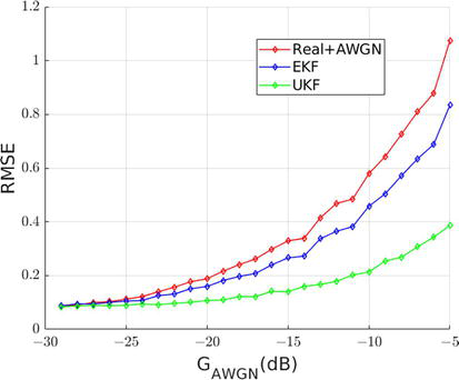
When performing a sweep in the gain of the noise added to the measurements of the Lidar and Radar sensors, and comparing the response of the EKF and UKF taking the RMSE as a reference parameter, the following response was observed.

Figure 8 shows a better capability of the UKF filter with respect to the EKF, for rejection of high noise levels in the sensor measurements, even when the noise level keeps increasing, the UKF response maintains low RMSE levels, i.e. it achieves a good estimation with respect to the real target position values. The following Table 1 shows the RMSE and MSE values for UKF and EKF with increasing AWGN. Note that the UKF response improves as the AWGN is increased.

Figure 8.

RMSE for EKF and UKF with increasing noise gain added to the dataset.

RMSE
G_AWGN	COORDINATE	EKF	UKF
−25dB	Px	0.1053	0.089
	Py	0.125	0.1
−20dB	Px	0.159	0.1073
	Py	0.1649	0.1166
−15dB	Px	0.266	0.14
	Py	0.2582	0.147
MSE
G_AWGN	COORDINATE	EKF	UKF
−25dB	Px	0.011	0.008
	Py	0.016	0.01
−20dB	Px	0.025	0.012
	Py	0.027	0.014
−15dB	Px	0.071	0.02
	Py	0.067	0.022

Table 1.

RMSE and MSE for X coordinate and Y coordinate.

Percentageally for −25 dB the UKF filter reduces noise by 14.8% more than the EKF filter, as the noise intensity is greater, this difference also increases with a value of 27.72% for −20 dB, and 38.23% at −15 dB.

4. Conclusions

For a correct filtering with EKF, good modeling of the system dynamics is required to achieve an accurate a priori prediction in the first stage of the filtering since the convergence of this filter by means of the Kalman gain is slower than the convergence of the UKF.

The UKF has a higher computational complexity compared to the EKF, when the CTRV model is combined with this last filter, a reduction of the computational complexity is obtained when it is implemented together with CORDIC.

When there is a fusion of Lidar and Radar sensor data in a drone with omnidirectional motion capability, the UKF filter has a better rejection of the noise associated with the measurements than the UKF filter.

Even with limited modeling of the system dynamics, the UKF manages to obtain an excellent response in the rejection of the noise associated with the fusion of the sensors.

By employing a progressive and constant increase of the distortion in the data obtained from the Lidar and Radar sensors, it was observed that the UKF has a more robust response to the increase of the uncertainty of the process to be filtered. For the actual implementation of a sensor data fusion system, this indicates a better adaptability of the UKF filter to different measurement scenarios as well as to differences in the quality of the sensors used.

Acknowledgments

The UPTC is part of the International Alliance with the Istituto di Tecnologie della Comunicazione dell’Informazione e della Percezione (TeCIP) from Italia and the Ljubljana University of Slovenia. We acknowledge NATO for the funds that make possible the research under grant G-5888 Science for Peace - Clarifier Research Project, and also, thanks to the UPTC for the administration of the funds under SGI-3139.

Conflict of interest

The authors declare no conflict of interest.