Distribution of Cortisol in Human Plasma in vitro: Equilibrium Solutions for Free Cortisol Using Equations of Mass Conservation and Mass Action

Abstract

Cortisol is secreted by the human adrenal cortex and circulates in plasma as free or protein-bound cortisol. Corticosteroid binding globulin (CBG) and albumin are the principal binding proteins (BPs) for cortisol in human plasma. Plasma concentrations of total cortisol (sum of protein-bound and free cortisol) are typically measured in vitro. Determination of free cortisol adds clinical and diagnostic value to total cortisol concentration. However, direct measurement of free cortisol concentrations involves laborious separation methods, limiting clinical utility. The development and application of physiologic protein-ligand binding models and equations provide an alternative approach to assessment of free cortisol concentrations in vitro. In this chapter, we introduce a matrix notation to represent relevant mass action and mass conservation equations. The matrix notation is also used to summarize and compare several contemporary models of interest, including cubic, quadratic, and quartic polynomial equations. Second, we introduce Feldman’s equations for competitive ligand-protein binding interactions, which are represented by matrices for multiple ligands and multiple BPs, including illustrative 2 × 2 matrix; we also discuss iterative solution strategies for coupled polynomial equations. Third, we develop a theorem for albumin-cortisol binding and review related assumptions that have been used to simplify polynomial equations and their equilibrium solutions.

1. Introduction

“A model should be as simple as it can be but no simpler.” Albert Einstein

“All models are wrong; some are useful.” George Box

1.1 Modeling the distribution of cortisol between free and protein-bound compartments in human plasma at equilibrium in the test tube (in vitro)

Several mathematical models have been put forward for the purpose of estimating equilibrium concentrations of free cortisol (X_F) in the test tube (in vitro). The minimum input data needed to estimate X_F include serum/plasma concentrations of total cortisol (X_TotF) and total corticosteroid binding globulin (X_TotCBG). Since X_TotF is known (measured experimentally), it is reasonable to consider that the problem is determining X_F as the fraction (or percentage) of the total cortisol, that is, (X_F/X_TotF). Though the clinician is primarily interested in free cortisol concentration (X_F), these polynomial models also yield estimates of CBG-bound (X_FC) and albumin-bound (X_FA) cortisol concentrations, which are generally of secondary interest.

1.2 Cortisol in captivity

Sampling of blood from the vascular volume by venipuncture is conventional and useful. Here we use in captivity in reference to the contained environment of the in vitro condition (and not in reference to BP-bound ligand as in Bikle et al. [1]). Once plasma/serum is removed from the well-mixed vascular compartment and placed in the test tube, there is no longer input or output of cortisol from the system; that is, in vitro rates of cortisol appearance, elimination, and diffusion are all zero. Moreover, X_TotF remains constant in the test tube; that is, dX_TotF/dt = 0 in vitro. By contrast, apart from the steady state, dX_TotF/dt ≠ 0 in vivo. We also note that the distribution of cortisol between free and protein-bound compartments quickly reaches equilibrium (or steady state) in vitro. A modeling perspective on the relationship between the dynamic and equilibrium conditions for cortisol in vitro is given in Appendix 1.

Thus, the in vitro assessment of cortisol captures a momentary snapshot or still life view of the dynamic, in vivo system. Despite these differences between the in vitro and in vivo conditions, analysis of cortisol distribution between free, CBG-bound, and albumin compartments in vitro yields information that can be usefully projected back to the dynamic model. This transition of parameters of interest from the in vitro equilibrium condition to the in vivo dynamic condition involves dividing association equilibrium constants into cognate on- and off-rate constants. Thus, the in vivo model uses on- and off-rate constants rather equilibrium association constants and differential equations (see [2]) rather than the iterative equilibrium equations discussed herein.

1.3 Motivations for estimating free cortisol concentrations by numerical modeling

Plasma or serum free cortisol concentrations (X_F) are generally difficult to measure, as they require pre-analytic separation procedures, such as equilibrium dialysis or ultrafiltration, at controlled temperature (37°C). These constraints have motivated interest in using numerical methods as an alternative approach to estimate X_F. Clinical laboratories routinely measure concentrations of total cortisol (X_TotF) and total albumin (X_TotA). Laboratory measurement of total CBG concentration (X_TotCBG) is less routine, but immunoassays are commercially available. In a typical scenario using contemporary methods, estimates of X_F can be obtained using a formula in which (i) X_TotF and X_TotCBG are measured, (ii) association rate constants are taken from the literature, and (iii) a value for albumin concentration is assumed (or measured) [3, 4].

In the present chapter we review equations for several contemporary models for estimation of X_F, including the cubic equation (Section 2) as well as quadratic and quartic polynomial equations (Section 3). These models all use principles of mass action and mass conservation. However, to the extent that they focus on cortisol to the exclusion of all other ligands that may compete for CBG and/or albumin binding, they may be regarded as too simple. In Section 4, we review the work of Feldman and co-workers [5, 6], which outline a system of integrated equations of mass action and conservation. These integrated equations can be applied to a variety of protein-ligand binding problems, including the binding of cortisol and other ligands to serum binding proteins (BPs), such as CBG and albumin. We shall refer to these as Feldman equations. We also introduce an alternative representation of Feldman equations using nxm matrix (K) notation. The matrix notation is introduced for the 3-compartment model (1 × 2, cubic solution) in Section 2.

1.4 Free, CBG-bound, and albumin-bound cortisol as a 3-compartment model

A minimal model for equilibrium solutions considers a single ligand (cortisol) and its two principal BPs in human plasma, namely CBG and albumin [2, 4, 7]. Whereas CBG-cortisol binding is specific, high-affinity, and saturable, albumin-cortisol binding is non-specific, low affinity, and non-saturable at physiologic concentrations of plasma cortisol [8]. The three compartments for cortisol in the vascular (plasma) volume (in vitro) include: (i) free (X_F), (ii) CBG-bound (X_FC), and (iii) albumin-bound (X_FA) cortisol (see Section 2). In this formulation, total cortisol represents the sum of three plasma compartments (X_TotF = X_F + X_FC + X_FA), illustrating the principle of mass conservation. An analytic solution (i.e., solution obtained using algebraic formula) for X_F may be obtained by a cubic equation, as previously described [4]. At a minimum, realistic modeling of cortisol distribution between free, CBG-bound, and albumin-bound compartments in vitro must take account of the different concentrations and binding characteristics of CBG and albumin. Thus, one- or two-compartment models may be too simple to realistically represent relevant physiology of cortisol in plasma and are not considered further in this chapter.

1.5 CBG-cortisol binding affinities are affected by temperature

CBG-cortisol binding affinity is sensitive to variation in temperature [9, 10, 11, 12, 13]. For purposes of this chapter, we focus on protein-ligand binding reactions at 37°C. In cortisol-binding studies performed using human serum at 37°C, values for the equilibrium dissociation constant for CBG-cortisol binding have been reported in the literature to be in the range of 12.5–33 nmol/L [3, 14, 15, 16, 17]. As temperature is increased from 37 to 40°C, CBG-cortisol affinity decreases substantially (by ≈50%) [9, 10, 11, 12, 13]. Thus, in febrile patients, free cortisol concentrations in vivo are expected to be greater than those (i) predicted by equations developed using affinity constants obtained for conditions at 37°C or (ii) measured experimentally at 37°C (e.g., by equilibrium dialysis).

1.6 Competitive protein-ligand binding models for multiple BP’s and multiple ligands

The problem of obtaining an accurate estimate of X_F becomes more challenging when one considers the possibility of other cortisol-binding proteins in human plasma, such as orosomucoid (α − 1-acidic glycoprotein, AAG) or elastase-cleaved CBG [18, 19, 20]. And the problem is compounded further considering the possibilities of ligands other than cortisol that circulate at sufficiently high concentration and bind CBG with sufficiently high affinity that, through their collective activities, they effectively compete with cortisol for CBG (and/or albumin) binding [14, 21, 22]. If ligands that effectively compete for CBG binding are not accounted for, model predicted X_F may significantly underestimate actual (experimentally measured) X_F. In Section 4 we review a generalized approach for modeling competition for CBG-cortisol (and albumin-cortisol) binding. These are represented by the 2 × 2 matrix, with several examples of ligands competing for CBG-cortisol binding reaction given in Section 5. Interestingly, once the Feldman equations are applied to two (or more) ligands, they are no longer tractable to analytic solutions. We discuss this problem of coupled polynomial equations and solution by iteration in Section 4. In Section 4, we also present Duality theorem that provides for transposition of matrix expression between n × m and m × n formats. We also provide theorems for existence and uniqueness of iterative solutions for the characteristic polynomial, which is developed more generally to existence and uniqueness of iterative solutions in Appendix 2. In Appendix 3, we further review matrix approaches to the characteristic polynomial, which includes use of singular value decomposition and vector-based matrix operations.

1.7 Re-parameterization of albumin-bound cortisol concentration (X_FA) results in simplifications to model equations and model solutions

Cortisol-albumin binding is characterized by low specificity and low affinity; moreover, since concentrations of albumin (μmol/L) greatly exceed those of cortisol (nmol/L), simplifications in modeling albumin-bound cortisol may be possible. Indeed, Tait and Burstein as well as Coolens and co-workers suggest that the concentration of albumin-bound cortisol (X_FA) is linearly related to X_F by a simple constant of proportionality (N) [3, 7]. By combining two parameters as a single parameter to estimate the concentration of X_FA, Coolens’ simplification reduces the order of the polynomial by one, such that analytic solutions using the cubic equation can now be obtained by a simpler (quadratic) equation (see Section 2). It may be noted that Coolens’ assumption only considers a single ligand (cortisol) binding to albumin. Since X_TotA >> X_TotF, the assumption that X_TotA ≈ ‘free albumin’ (X_A) seems reasonable enough. However, when one considers the myriad other ligands that bind albumin in non-specific fashion, the assumption that X_TotA ≈ X_A is less certain. A general theorem for albumin-cortisol binding, by which multiple ligands may compete for albumin-cortisol binding, is developed in Section 6. These considerations also raise the practical question of whether N is in fact constant (within and between individuals) and exactly what value of N should be used as the constant of proportionality (X_FA/X_F).

It also is uncertain whether there is a single or multiple cortisol binding sites per albumin molecule. In Appendix 4, we use the matrix format to represent equations for multiple albumin-cortisol binding sites having different but independent cortisol binding affinities.

1.8 The clinical conundrum

One might imagine that having measured concentrations of X_TotF, X_TotCBG, and X_TotA in hand, estimation of X_F (as a percent of X_TotF) should be a simple enough task. After all, cortisol binds CBG with simple 1:1 stoichiometry and the binding properties of CBG and cortisol are well characterized [10, 15, 16, 23, 24, 25, 26]. Similarly, purified albumin is readily available and cortisol binding properties have been reported [4, 17, 27, 28, 29, 30]. For example, in Section 6 we review albumin-cortisol binding data obtained in a purified solution of human serum albumin [27].

However, we find in practice that estimation of X_F in human plasma using contemporary models remains an inexact science. These model solutions for X_F often match experimentally measured free cortisol; however, their performance may be inconsistent in certain individuals, populations, and conditions. Changing affinities and variation in concentrations of competing ligands in conditions such as critical illness and septic shock may further challenge clinical application of contemporary numerical methods to estimate X_F.

Before introduction to the n × m matrix notation for Feldman equations, let us briefly review our use of the terms equilibrium concentration and bioavailable cortisol.

1.9 Definition of equilibrium concentrations in the test tube (which is a thought experiment)

To be clear about what is meant by the term equilibrium (or steady state) solutions in vitro, let us consider as a thought experiment a sample of human plasma having median normative concentrations of CBG and albumin from which cortisol has been removed (e.g., by charcoal adsorption). Thus, in this theoretical plasma sample CBG ≈ 600 nmol/L, albumin ≈ 600,000 nmol/L, and total cortisol = 0 nmol/L. To 0.1 mL of this sample, let us add 1 μL of (free) cortisol at a concentration of 10,000 nmol/L, which when diluted in the 100 μL sample volume yields a final total cortisol concentration of ≈100 nmol/L after mixing. Immediately following addition of (free) cortisol to the sample, there is a (brief) dynamic phase during which concentrations of X_F, X_FC, and X_FA are rapidly changing. A new steady state is quickly achieved in the test tube, after which period concentrations of X_F, X_FC, and X_FA (in the test tube) remain constant. Modeling studies suggest that steady state occurs rapidly in this example [4]. When we speak of equilibrium solutions, we are referring to cortisol concentrations at these equilibrium (or steady state) conditions. See Appendix 1 for further discussion of dynamic and steady state conditions in vitro.

1.10 Parsing the problem: bioavailable cortisol (X_F + X_FA)

In studies of in vitro testosterone distribution among free (X_T), SHBG-bound (X_TS), and albumin-bound (X_TA) testosterone compartments, X_TS can be separated from X_T and X_TA by ammonium sulfate precipitation. The term bioavailable testosterone has been commonly used to denote the non-SHBG-bound fraction of testosterone (i.e., free and albumin-bound testosterone), where X_TotT = X_T + X_TS + X_TA and bioavailable testosterone (T_bioavail) = (X_TotT – X_TS) = (X_T + X_TA). In the present chapter, we use the term bioavailable cortisol (F_bioavail) to denote the sum of free and albumin-bound cortisol (X_F + X_FA). Our use of the term is restricted to these concentrations without any intended endorsement of proposed biological activity of albumin-bound cortisol related to capillary transit times [31, 32, 33, 34]. In fact, from a modeling perspective of systemic concentrations of cortisol in vivo, X_FA does not diffuse between vascular and extravascular compartments; rather, X_FA varies in time-dependent fashion in dynamic equilibrium with X_F and X_FC (in the plasma compartment) [2, 8, 35]. Nonetheless, the concept of bioavailable cortisol may be useful to cortisol in vitro, as it parses the problem of estimating free cortisol into two tasks. The first task is determination of the concentration of bioavailable cortisol as a fraction of (measured) total cortisol (X_TotF), where bioavailable cortisol = (X_TotF – X_FC) = (X_F + X_FA). Once bioavailable cortisol concentration has been determined, the second task is selecting the correct constant of proportionality (N = X_FA/X_F) by which bioavailable cortisol can be apportioned between X_F and X_FA fractions.

2. Matrix notation for cubic equation (1 × 2 matrix)

A simple formulation of the nxm matrix shown in Table 1 includes free ligand (row), free concentrations of BPs (columns), and protein-bound cortisol concentrations (inner cells). The principle of mass action is represented by the 1:1 stoichiometric formulae in each inner cell in the matrix, where concentrations of CBG-bound cortisol (FC) and albumin-bound cortisol (FA) are expressed as mass action formulae using equilibrium association constants for CBG-cortisol ($K_{11}$) and albumin-cortisol ($K_{12}$) binding reactions at 37°C. For example, the inner cell for steady state concentration of FC (dotted ellipse) is the product of (i) molar concentrations of the reactants, free cortisol (F) and free CBG (C), and (ii) the equilibrium association (affinity) constant for CBG-cortisol binding ($K_{11}$). Note that the equilibrium association constant is expressed in units of concentration⁻¹ (L/nmol, nM⁻¹). Thus, inner cell entries are of the form $K_{11}·C·F$. By the same token, the inner cell for steady state (equilibrium) concentration of albumin-bound cortisol (FA) in vitro at 37°C (dashed ellipse) is the product of (i) molar concentrations of the reactants, free cortisol (F) and free albumin (A), and (ii) the equilibrium association (affinity) constant for albumin-cortisol binding ($K_{12}$). Thus, inner cell entries for albumin-cortisol binding are in the form $K_{12}·A·F$. In Table 1 and elsewhere, we designate the equilibrium affinity constant for CBG-cortisol binding as $K_{11}$ and the equilibrium affinity constant for albumin-cortisol binding as $K_{12}$.

Table 1.

Tutorial 1 × 2 matrix for cortisol binding equilibrium equations resulting in a cubic solution for free cortisol.

The three total concentrations are: total cortisol (TotF), total CBG (TotC), and total albumin (TotA) are measured (light red). The affinity constants for CBG-cortisol (K₁₁) and albumin-cortisol (K₁₂) binding are obtained from the literature or otherwise estimated (yellow). The free cortisol concentration (F) is estimated as cubic solution derived from the equilibrium equations of Feldman and co-workers [5] (light blue). The dashed boxes and ellipses are in this table to illustrate the discussion in the text. Briefly, ellipses enclose the mass action formulae for cortisol binding to CBG and albumin. Boxes enclose conservation of mass formulae. The horizontal box (dotted rectangle) indicates that total cortisol (TotF) represents the sum free (F), CBG-bound (FC), and albumin-bound (FA) cortisol. The vertical box (compound dashed rectangle) indicates that total CBG (TotC) represents the sum of free CBG (C) and cortisol-bound CBG (FC). The dashed box indicates that total albumin (TotA) represents the sum of free albumin (A) and cortisol-bound albumin (FA). Feldman equations give a solution of free F as a root of a cubic polynomial [4].

Constraints: None.

Although the equilibrium affinity (association) constants for CBG-cortisol (K₁₁) and albumin-cortisol (K₁₂) binding reactions are useful in the matrix notation, in other circumstances it may be preferable to consider the reciprocal, i.e. the equilibrium dissociation constant (K_d). We use the term K₁₁⁻¹, which is also equal to 1/$K_{11}$, to indicate the equilibrium dissociation constant for CBG-cortisol binding. Similarly, we use the term K₁₂⁻¹, which is equal to 1/$K_{12}$, to indicate the equilibrium dissociation constant for albumin-cortisol binding reaction. Note that equilibrium dissociation constants are expressed in more familiar units of concentration (nmol/L). Values abstracted from Coolens’ quadratic equation reflect the high affinity of CBG-cortisol binding (K₁₁⁻¹ = 33 nmol/L) and relatively low affinity (K₁₂⁻¹ = 330,000 nmol/L) of albumin-cortisol binding (assuming 1:1 stoichiometry).

The principle of mass conservation is also illustrated in Table 1. For example, total concentrations of ligand (row sums, dotted rectangle) and BP (column sums, compound dash and dashed rectangles), are shown in right and bottom margins, respectively. Note that in the usual application of the equations, which is to obtain an analytic solution (i.e., a solution that can be obtained by algebraic formula) for X_F, total concentrations of ligand and BPs are typically measured (red), while equilibrium affinity constants, K₁₁ and K₁₂ for CBG- and albumin-cortisol binding, respectively, are taken from literature (yellow). In the example shown in Table 1, total cortisol, total CBG, and total albumin are measured (red); K₁₁ and K₁₂ are taken from the literature (yellow); and free cortisol concentration is solved (blue) by the cubic equation. As noted in Coolens et al. and elsewhere [3, 4, 25, 36, 37], the assumption that given value for K₁₁ is broadly applicable across individuals, conditions, and clinical groups, may be inaccurate. For example, genome-wide association studies [36, 38] and the presence of recognized polymorphisms of CBG having reduced cortisol binding affinity in certain populations [25, 39] demonstrate that some individuals have normal concentrations of CBG, when measured by immunoassay, but reduced cortisol binding affinity. Individual differences in glycosylation of CBG may also influence its cortisol binding affinity, as do specific mutations associated with the syndrome of CBG deficiency [40, 41, 42].

3. Other models that treat cortisol as the sole ligand involved in protein binding in human plasma/serum (quadratic and quartic solutions)

In addition to the cubic equation described in Table 1, several variations on the basic cubic model have been suggested in the literature. Note that like the cubic equation, these variations also consider cortisol to be the sole ligand involved in protein-binding reactions. As a result, like the cubic equation, the corresponding solutions for X_F are polynomial equations that yield analytic solutions (quadratic solution for Coolens’ equation and quartic solution for the model proposed by Nguyen et al. [3, 20].

Coolens’ quadratic equation (Table 2) can still be represented as a 1 × 2 matrix. However, in Coolens’ equation, the mass action term for X_FA in the cubic equation (dashed oval in Table 1) is re-parameterized such that (K₁₂A*F) is simplified to (N*F). In this formulation, N = X_FA/X_F = K₁₂*A ≈ K₁₂*X_TotA. Coolens’ formula takes a value for equilibrium dissociation constant for albumin-cortisol binding from the literature (= 330,000 nmol/L) and assumes a normative value for serum albumin concentrations, yielding N = 1.74 [3]. The quadratic equation can be represented in matrix format as shown in Table 2. In Coolens’ formulation, N is viewed as proportional to the concentration of total albumin concentration (X_TotA), and in adaptations of Coolens’ equation the value of N has been adjusted proportionately to measured X_TotA [3, 43]. The assumptions related to Coolens’ equation and a general theorem to handle competition of multiple ligands for albumin-cortisol binding are further developed in Section 7 below.

Table 2.

1 × 2 matrix for cortisol binding equilibrium equations resulting in Coolens’ quadratic solution.

The solution for free cortisol proposed by Coolens et al. [3] is obtained under a constraint that F is small (see constraint listed below) [3, 7]. Coolens’ constant N replaces $K_{12}A$in the mass action formula to obtain the cell entry N·F. Coolens’ assumption listed under constraints below for the 1 × 2 matrix implies A = TotA. The conservation of mass equation for TotF leads to Coolens quadratic solution for the free concentration F. Coolens solution gives N = 1.74, but other values are possible [3].

Constraints: Coolens assumption $K_{12}F$ <<1; that is, F < < $K_{12}^{-1}=K_D,$the equilibrium dissociation constant of cortisol-albumin binding.

Note that Coolens’ simplification provides a simpler (quadratic) solution when compared to the cubic equation (Table 1). This is accomplished by combining X_F + N*X_F = (1 + N)X_F and deleting the column for X_A. This results in a 1 × 1 matrix table and a quadratic solution. For further discussion of the degree of polynomial equations, see Section 3 and Appendix 3.

3.1 Quartic solution

The quartic solution [20] adds a third column to the cubic solution for the additional binding protein, elastase-cleaved CBG (C_e), resulting in 1 × 3 matrix (see Table 3). Gudman-Hoeyer and Ottesen further developed the quartic model to consider multiple ligands and dynamical rates of appearance and elimination of elastase-cleaved CBG [19]. However, the clinical relevance of the quartic model is uncertain, especially in view of reports by Hammond and co-workers that the identification of a putative low-affinity (elastase-cleaved) CBG using the 9G12 monoclonal antibody was related to experimental artifact [40]. Moreover, it appears that elastase-cleaved CBG is rapidly cleared at local sites of inflammation, such that systemic serum concentrations of elastase-cleaved CBG are unmeasurably low [41].

Table 3.

1 × 3 matrix for equilibrium equations including elastase-cleaved CBG.

For this matrix, two forms of CBG having distinct cortisol binding affinities are proposed to exist: (i) full length CBG (C) and (ii) elastase-cleaved CBG (${\mathrm{C}}_{\mathrm{e}})$.The four total concentrations are total cortisol (TotF), total CBG (TotC), total elastase-cleaved CBG (Tot$C_e$), and total albumin (TotA) are measured (light red). The affinity constants for free cortisol binding to intact CBG (K₁₁), to elastase-cleaved CBG (K₁₃), and to albumin (K₁₂) are obtained from the literature or otherwise estimated (yellow) [19, 20]. The free cortisol concentration (F) is estimated as the root of a quartic polynomial as described in Nguyen et al. [20] (light blue).

Constraints: None, or in some cases that Tot $C_e$ equals a fixed fraction of TotC.

Quartic solution including addition binding protein (α1-acidic glycoprotein, AAG) (1 × 3 matrix) (Table 4): In addition to CBG and albumin, α₁-acid glycoprotein (AAG), also known as orosomucoid, circulates in human plasma at a mean concentration of ≈24 μM and binds cortisol with an affinity (K_D = 62,000 nM) intermediate to CBG (K_D = 33 nM) and albumin (K_D = 330,000 nM) [18, 44]. Table 4 shows a 1 × 3 matrix that includes AAG as an additional binding protein. The concentration of AAG-bound cortisol under physiologic conditions appears to be small [19]. However, depending on the concentration of AAG and other ligands that compete with cortisol for AAG-binding, it may contribute significantly to the pool of protein-bound cortisol. AAG may also represent an additional source of saturable cortisol-binding under conditions, such as CBG deficiency or low CBG concentrations [27]. As illustrated in Table 4, it is the concentration of free rather than total AAG that determines the concentration of AAG-bound cortisol. Considering the variety of other ligands that bind AAG, concentrations of free AAG (X_AAG) may be substantially reduced relative to total AAG (X_TotAAG), as discussed further in the general theorem (2 × 2 matrix) for albumin-cortisol binding (Section 7).

Table 4.

1 × 3 matrix for equilibrium equations including orosomucoid (AAG).

An alternative model includes orosomucoid (α − 1-acidic glycoprotein, AAG) as an additional cortisol-binding protein [44]. The four total concentrations are total cortisol (TotF), total CBG (TotC), total orosomucoid (TotO) and total albumin (TotA) are measured (light red). The affinity constants for CBG-cortisol (K₁₁), albumin-cortisol (K₁₂), and orosomucoid-cortisol (K₁₃) binding are obtained from the literature or otherwise estimated (yellow). The free cortisol concentration (F) is estimated as a root of a quartic polynomial (light blue).

Constraints: None.

Degrees of characteristic polynomials: In the above examples (single ligand, multiple BPs), note that each additional column adds one additional order of complexity to the polynomial equations; by contrast, treatment of albumin-cortisol binding as a constant (N) reduces the order of the polynomial by one. The degree of characteristic polynomials is discussed further in Appendix 3.

Also note that all the models discussed thus far consider cortisol as the sole ligand; that is, there is only one row (for cortisol only) in the n × m matrix. Consequently, analytic solutions may be obtained by algebraic equations, such as the familiar quadratic, cubic, quartic solutions discussed above. However, when there are two or more ligands competing for protein binding, a more complex system of coupled polynomial equations obtains. These coupled polynomial equations do not yield simple analytic solutions; rather they require iterative procedures to obtain solutions [19, 45, 46]. For these problems, a more general approach taking advantage of mass action and mass conservation equations has been developed.

4. Competitive ligand-protein binding equilibrium equations (for two or more ligands, 2 × 2 matrix) require iterative rather than analytic solutions

Feldman’s system of coupled equilibrium equations obtained from mass action and mass conservation equations is developed here in a matrix format for one or more ligands and one or more binding proteins [5, 6]. This will be done for n ligands and m binding proteins; however, the case n = 2 and m = 2, the 2 × 2 matrix, conveys the principles needed.

To simplify the discussion, consider the equilibrium of free cortisol concentration ($F$) binding to free CBG ($C$) and free albumin $\left(A\right)$ as well as a known competitor ($P$) that also binds to CBG and albumin. This equilibrium can be represented in matrix format for a 2 × 2 matrix of affinities $\left[K_{\mathit{ij}}\right]$ extended to include the free concentration on the left and top margins and total concentrations on the right and bottom margins (Table 5). Note that it is the matrix of affinities $\left(K_{\mathit{ij}}\right)$ that is 2 × 2. Also note that the bounded concentrations $X_{\mathit{FC}}$, $X_{\mathit{FA}}$, $X_{\mathit{PC}}$, and $X_{\mathit{PA}}$ have been replaced by mass action formula (assuming 1:1 stoichiometric binding). The four total concentrations give rise to four non-linear equations and, assuming total concentrations and all affinities $K_{\mathit{ij}}$ are known, we have four equations for the four free concentrations: F (free cortisol), P (free competitor), C (free CBG), and A (free albumin).

Table 5.

2 × 2 matrix for competitive ligand binding equilibrium equations with two ligands (cortisol and competitor (P)) that both bind CBG (and albumin) (iterative solution).

This 2 × 2 matrix illustrates equilibrium with multiple ligands and multiple binding proteins. The four total concentrations (total cortisol (TotF), total competitor ligand (TotP), total CBG (TotC), and total albumin (TotA)) are measured (light red). The affinity constants for CBG-cortisol (K₁₁) and albumin-cortisol (K₁₂) binding are obtained from the literature or otherwise estimated (yellow). Assuming P is a specific ligand, the affinities (K₂₁) and (K₂₂) are also obtained from the literature (yellow). The free cortisol (F) and free competitor (P) concentrations are estimated by iteration of the equilibrium equations described by Feldman et al. [5] (light blue).

To explain: the solutions of free F and P are both a positive root of a cubic equation. However, the two cubic equations are coupled (the coefficients of one equation requires knowing the solution of the other), so F and P need to be solved simultaneously. There is no analytic solution by algebraic methods, but solutions can be obtained by iteration.

Constraints: None.

This matrix is both a visual aid and a computation aid. The conservation of mass equations are derived as row sums of the free concentration on extreme left plus the cell entries to obtain the total concentration in the right margin:

$$\begin{array}{l}\mathit{Tot}F=F\left(1+K_{11}C+K_{12}A\right)\\ \mathit{Tot}P=P\left(1+K_{21}C+K_{22}A\right);\text{and}\text{as}\end{array}$$E1

column sums of the free concentration on extreme top plus the cell entries to obtain the total concentration in the bottom margin:

$$\begin{array}{l}\mathit{Tot}C=C\left(1+K_{11}F+K_{21}P\right)\\ \mathit{Tot}A=A\left(1+K_{12}F+K_{22}P\right)\end{array}$$E2

The mass action equilibrium equations are represented as the cell entries in above matrix; for example, the CBG-bound cortisol concentration X_FC is entered as $K_{11}·F·C$ in the 1,1 (upper left-hand corner cell).

Note that these 1:1 stoichiometric mass action formulae allow the F to be factored out of the first row sum for Free F, with similar operations for all of the marginal sums giving a very convenient form for all four conservation of mass formulae above. For example, Feldman’s 1972 iterative equations [5], for this case, are now easily derived from the systems of Eqs. (1) and (2) by cross dividing to obtain the system of iterative equations Eqs. (3) and (4):

$$\begin{array}{l}F=\frac{\mathit{\text{TotF}}}{\left(1+K_{11}C+K_{12}A\right)}\\ P=\frac{\mathit{\text{TotP}}}{\left(1+K_{21}C+K_{22}A\right)}\end{array}$$E3

where

$$\begin{array}{l}C=\frac{\mathit{\text{TotC}}}{\left(1+K_{11}F+K_{21}P\right)}\\ A=\frac{\mathit{\text{TotA}}}{\left(1+K_{12}F+K_{22}P\right)}.\end{array}$$E4

We call these iterative equations because guessing initial values for C and A, we can compute F and P (the first iteration); then with F and P we can compute C and A and then recompute F and P (the second iteration); and so on. A stopping rule can be defined as when F and P stop changing within specified limits.

Feldman et al. also continues this development by substituting the formulas for C and A into the equations for F and P [5] to obtain their Eq. (25). They are complicated equations but do show that the iterative equations can be written in terms of F and P alone. It will be somewhat simpler if we substitute the formulas for C and A into our original version of the F equation Eqs. (1) and (2) above, considering the P equation as a nuisance; that is, focusing on F and its equation. We have

$$\mathit{Tot}F=F\left(1+\frac{K_{21}\mathit{\text{TotC}}}{\left(1+K_{11}F+K_{21}P\right)}+\frac{K_{22}\mathit{\text{TotA}}}{\left(1+K_{12}F+K_{22}P\right)}\right)$$E5

This suggests that the iterative solution might be computed as the roots. Roots refer to the solutions of the polynomial equations (polynomial set equal to zero). The characteristic polynomial is obtained by algebraically clearing fractions in Eq. (5).

To be clear about this, define the product

$$\mathrm{\Pi }=\left(1+K_{11}F+K_{21}P\right)\left(1+K_{12}F+K_{22}P\right)=\left(K_{11}F+C_{21}\right)\left(K_{12}F+C_{22}\right),$$

where $C_{21}=1+K_{21}P\mathit{\text{and}}{C}_{22}=1+K_{22}P,\mathit{\text{both}}>1.$ $\mathit{\text{and}}\mathit{are}\mathit{\text{constant with respect to}}F.$ Multiplying both sides of (5) by Π clears the fractions and gives

$$\mathit{Tot}F·\mathrm{\Pi }=F·\mathrm{\Pi }+K_{21}\mathit{\text{TotC}}·\left(K_{12}F+C_{22}\right)+K_{22}\mathit{\text{TotA}}·\left(K_{11}F+C_{21}\right)$$E6

So, $\mathrm{\Pi }$is a quadratic polynomial and $F·\mathrm{\Pi }$ is a cubic polynomial and the other terms give linear polynomials or constants. This Eq. (6) is the cubic polynomial such as obtained in Dorin et al. [4] where there was no P and $C_{21}=C_{22}=1$. The standard solution of the cubic equation given in [4] and given more generally here shows existence of a solution. Also, for plausible values of F and P, the standard solution of the cubic equation can show uniqueness of the solution.

Comments. We have focused on the equation for F, but we can repeat Eqs. (5) and (6) for P. We then have two polynomial equations. We should also mention an important duality; we could write equations like Eqs. (5) and (6) for free A and C and iterate to find the solutions for A and C first, then one step computations using Eq. (3) would give us F and P. Usually, we do not care about A and C, but you could solve for A and C first and then compute F.

The problem with this approach in the above comment is that the polynomials for F and P are coupled; that is, the coefficients of the F polynomial are functions of P and the coefficients of the P polynomial are functions of F. For example, the 1 × 2 matrix results is a cubic polynomial for which we can compute the positive root since there is only one equation and no coupling. But for the 2 × 2 matrix there is coupling and we cannot solve the positive root because the coefficients are unknown since they are functions of the unknown P. Thus, we continue to need to find ligand-protein binding equilibrium solution values iteratively. Both Mazer [45] as well as Gudmand-Hoeyer and Ottesen [19] treat 2 × 2 cases but iterate to find solutions, as did and Rohatagi et al. for competition of prednisolone and cortisol for CBG binding [46].

None-the-less, we wish to save this duality theorem; it is true here and in general, so we will wait until the next section to write it down.

4.1 Generalization to n × m matrix representation of the equilibrium equations

The generalization of the equilibrium equations from the above case for 2 × 2 matrix to the n × m matrix is straightforward just with a cost of more notation. We use the notation system of Feldman et al. [5] where free hormones (ligands) were designated P₁, P₂, …, P_n and binding proteins were designated as Q₁, Q₂, …, Q_m and represent these equations in a matrix format, as shown in Table 6.

Matrix n × m	$Q_1$	$\cdots$	$Q_j$	$\cdots$	$Q_m$
$P_1$	$K_{11}{P}_1{Q}_1$	$\cdots$	$K_{1j}{P}_1{Q}_j$	$\cdots$	$K_{1m}{P}_1{Q}_m$	${\mathit{\text{TotP}}}_1$
$\cdots$	$\cdots$		$\cdots$		$\cdots$
$P_i$	$K_{i1}{P}_i{Q}_1$	$\cdots$	$K_{\mathit{ij}}{P}_i{Q}_j$	$\cdots$	$K_{\mathit{im}}{P}_i{Q}_m$	${\mathit{\text{TotP}}}_i$
$\cdots$	$\cdots$		$\cdots$		$\cdots$
$P_n$	$K_{n1}{P}_n{Q}_1$	$\cdots$	$K_{\mathit{nj}}{P}_n{Q}_j$	$\cdots$	$K_{\mathit{nm}}{P}_n{Q}_m$	${\mathit{\text{TotP}}}_n$
	${\mathit{\text{TotQ}}}_1$	$\cdots$	${\mathit{\text{TotQ}}}_j$	$\cdots$	${\mathit{\text{TotQ}}}_m$

Table 6.

General n × m matrix.

The total concentrations ${\mathit{\text{TotP}}}_i$ and ${\mathit{\text{TotQ}}}_j$ are measured and the nxm matrix of association constants $K=\left[K_{\mathit{ij}}\right]$ are known. The concentrations of free ligands $P=\left[P_i\right]$ are to be estimated. The mass conservation equations for the n rows and m columns together with mass action formulae yield Feldman’s iterative equations that solve for free ligand concentrations P in left margin column [5].

So, the conservation of mass equation for the concentration $\left[{\mathit{\text{TotP}}}_i\right]$ is the sum of the ith row:

$$\mathit{Tot}{P}_i=P_i+P_i{Q}_1+\cdots +P_i{Q}_j+\cdots +P_i{Q}_m=P_i+\sum _{j=1}^m{P}_i{Q}_j$$

Note that Feldman et al. [5] and we assume univalent (stoichiometric) binding for the ligand-protein binding reaction $P_i+Q_j\rightleftharpoons P_i{Q}_j$ in equilibrium. So, the mass action equilibrium gives $P_i{Q}_j=K_{\mathit{ij}}·P_i·Q_j$ where $K_{\mathit{ij}}$ is the association constant (affinity) of this reaction.

Thus, the sum in the ith row becomes

$$\mathit{Tot}{P}_i=P_i+\sum _{j=1}^m{K}_{\mathit{ij}}·P_i·Q_j=P_i\left(1+{\sum }_{j=1}^m{K}_{\mathit{ij}}{Q}_j\right)$$E7

which generalizes Eq. (1) above and with similar expressions generalizing Eq. (2) yields the general Feldman’s iterative equations

$$P_i=\frac{\mathit{Tot}{P}_i}{\left(1+{\sum }_{j=1}^m{K}_{\mathit{ij}}{Q}_j\right)}$$E8

with

$$Q_j=\frac{\mathit{Tot}{Q}_j}{\left(1+{\sum }_{i=1}^n{K}_{\mathit{ij}}{P}_i\right)}.$$E9

Though the Feldman equilibrium equations treated iteratively have been used to obtain equilibrium solutions of free ligand concentrations (P’s) [5, 6, 19, 45], it would be helpful to consider existence and uniqueness of these solutions more generally. Thus, we continue the development. The generalization of Eq. (5) is

$$\mathit{Tot}{P}_i=P_i\left(1+{\sum }_{j=1}^m\frac{K_{\mathit{ij}}{\mathit{\text{TotQ}}}_j}{\left(1+{\sum }_{i=1}^n{K}_{\mathit{ij}}{P}_i\right)}\right)$$E10

Before continuing this discussion, let us give the Duality theorem here.

4.2 Duality theorem for equilibrium matrix K

The transpose (reverse rows and columns) of the equilibrium table for the nxm matrix K gives an equivalent equilibrium table for the mxn matrix $K^T$. The solution(s) of the dual matrix (table) are the same as for the original matrix.

Proof. Instead of solving for $P_i$ first as in Eq. (10), it is equally possible to write the analogous equations for $Q_j$, solve for the $Q_j$ first and then solve for the $P_i$ second using Eq. (8). In terms of the K matrix table we only need to reverse rows and columns, that is, use the matrix transpose $K^T$.

Continuing the discussion of Eq. (10), a relatively simple presentation of our system of coupled polynomials is obtained by clearing fractions where possible in Eq. (10). So, define

$\mathrm{\Pi }={\prod }_{j=1}^m\left\{1+{\sum }_{k=1}^n{K}_{\mathit{kj}}{P}_k\right\}={\prod }_{j=1}^m\left\{K_{\mathit{ij}}{P}_i+1+{\sum }_{k\ne i}{K}_{\mathit{kj}}{P}_k\right\}={\prod }_{j=1}^m\left\{K_{\mathit{ij}}{P}_i+C_{\mathit{ij}}\right\}$ where $C_{\mathit{ij}}=1+{\sum }_{k\ne i}^m{K}_{\mathit{kj}}{P}_k>1$ and is constant with respect to$P_i.$

Note that ${\prod }_{j=1}^m\left\{K_{\mathit{ij}}{P}_i+C_{\mathit{ij}}\right\}$ could be expanded (analogous to the binomial theorem) as a sum of terms$,$ which is a m-degree polynomial in $P_i$provided all $K_{\mathit{ij}}>0;$ and the constant term of this polynomial is ${\prod }_{j=1}^m{C}_{\mathit{ij}}$ > 1.

So, clearing of fractions in Eq. (10) by multiplying both sides by Π yields

$$\mathrm{\Pi }{P}_i+\sum _{j=1}^m{K}_{\mathit{ij}}\mathit{Tot}{Q}_j{P}_i\prod _{\nu \ne j}\left\{K_{\mathit{i\nu }}{P}_i+C_{\mathit{i\nu }}\right\}=\left(\mathit{Tot}{P}_i\right)\mathrm{\Pi }$$E11

Comment. Each Π in Eq. (11) is a polynomial where $\mathrm{\Pi }{P}_i$is a m + 1 degree polynomial and the $P_i{\prod }_{\nu \ne j}$ are m-degree polynomials; and the linear combination of polynomials is a polynomial. Thus Eq. (11) is a (m + 1) degree polynomial equation in $P_i$, provided all $K_{\mathit{ij}}>0$. (If a $K_{\mathit{ij}}=0$, then the degree is reduced by 1, that is, the degree of the polynomial Eq. (11) equals the number of non-zero $K_{\mathit{ij}}$ plus 1.)

4.3 Existence theorem for characteristic polynomial

Eq. (11) for $P_i$ has at least one positive solution.

Proof. Eq. (11) for $P_i$ as a (m + 1) degree polynomial in each $P_i$ can be written as $A_{m+1}{P}_i^{m+1}+A_m{P}_i^m+\cdots +A_1{P}_i^1+\mathrm{C}=0,$ where $C=-\left(\mathit{Tot}{P}_i\right){\prod }_{j=1}^m{C}_j<-\mathit{Tot}{P}_i<0$ and $A_{m+1}={\prod }_{\nu =1}^m{K}_{\mathit{i\nu }}>0.$

Descartes’ Rule of Signs for polynomials says the number of positive roots is related to the number of sign changes of the coefficients of the polynomial. For our (m + 1) degree polynomial, there is at least one sign change regardless of whether coefficients $A_2\cdots A_{m+1}$ are positive or negative or zero. This implies there is at least one positive solution for $P_i$; that is, existence of a solution is shown. Additional discussion of Descartes’ Rule of Signs and analysis of the existence theorem is presented in Appendix 2.

4.4 Uniqueness theorem for characteristic polynomial

Eq. (11) for $P_i$ has exactly one positive solution.

Proof. To show uniqueness of a positive root of the characteristic polynomial known to exist, we return to the way we obtained this characteristic polynomial. To clear fractions, we multiplied Eq. (10) by $\prod ={\prod }_{j=1}^m\left\{K_{\mathit{ij}}{P}_i+C_{\mathit{ij}}\right\}$. Since the characteristic polynomial is product of two functions, the roots of this polynomial are the sum (union) of the roots of each factor. Now the m roots of ∏ are all negative. The second factor coming from Eq. (10) is

$$\begin{array}{l}{P}_i\left(1+{\sum }_{j=1}^m\frac{K_{\mathit{ij}}{\mathit{\text{TotQ}}}_j}{\left(1+{\sum }_{i=1}^n{K}_{\mathit{ij}}{P}_i\right)}\right)-\mathit{Tot}{P}_i.\text{As}\text{developed}\text{above}\text{this}\text{becomes}\\ P_i\left(1+\sum _{j=1}^m\frac{K_{\mathit{ij}}{\mathit{\text{TotQ}}}_j}{\left(K_{\mathit{ij}}{P}_i+C_{\mathit{ij}}\right)}\right)-\mathit{Tot}{P}_i=\sum _{j=1}^m\frac{{\mathit{\text{TotQ}}}_j{P}_i}{\left(P_i+B_{\mathit{ij}}\right)}-\left(\mathit{Tot}{P}_i-P_i\right)\text{where}{B}_{\mathit{ij}}=\frac{C_{\mathit{ij}}}{K_{\mathit{ij}}}.\end{array}$$

Next, $P_i\mathit{\text{and}}\frac{P_i}{\left(P_i+B_{\mathit{ij}}\right)}$ are monotone increasing functions of $P_i$, so their sum (this factor) is also. Now free $P_i$ satisfies $0\le P_i\le \mathit{Tot}{P}_i.$So evaluating the second factor at each end point, we have at $P_i=0,$ $\text{factor}=-\mathit{Tot}{P}_i$ which is negative and at $P_i=\mathit{Tot}{P}_i$, $\text{factor}={\sum }_{j=1}^m\frac{{\mathit{\text{TotQ}}}_j\mathit{Tot}{P}_i}{\left(\mathit{Tot}{P}_i+B_{\mathit{ij}}\right)}$ which is positive. This implies there is exactly one root (a positive root). Thus, the characteristic polynomial is the product of two factors and has m negative roots and exactly one positive root. This is a proof of uniqueness.

Comment. One might say the proof of existence given above is not needed, since the proof of uniqueness given here does both existence and uniqueness. Nonetheless, we needed the detailed development of the characteristic polynomial and the expanded discussion of this was instructive (also see Appendix 2).

5. Clinical correlates of competition for CBG-cortisol binding

In discussing limitations of their proposed method of calculating free cortisol, Coolens et al. acknowledge that cortisol-binding affinity of CBG may vary between individuals [3], which has been confirmed in subsequent studies [36, 39, 47]. They also noted the potential role of other ligands that compete for CBG-cortisol binding: “The fact that only the interaction of cortisol with CBG is taken into consideration constitutes a second limitation. In some conditions, significant amounts of other steroids may interfere with this equilibrium. This will be the case during pregnancy and also for patients with congenital adrenal hyperplasia… the proposed method cannot be applied to umbilical cord blood, and in congenital adrenal hyperplasia [3]”. Thus, although CBG binds cortisol with specificity, there are several other steroid compounds that bind CBG with significant affinity. If the free concentrations of these CBG-binding ligands are sufficiently high in the test tube, they can effectively compete with CBG-cortisol binding and raise the equilibrium concentration of X_F. CBG is also the transport globulin for progesterone, which binds CBG with 3-fold lower affinity than cortisol and at high concentrations of (free) progesterone can effectively compete in the CBG-cortisol binding reaction. For example, as described by Hodyl et al. very high progesterone concentrations in fetal cord blood are capable of elevating free cortisol concentrations through competition with cortisol at CBG’s hormone binding site. This competition raised X_F without CBG cleavage or altered CBG hormone-binding affinity [21]. Similar results demonstrating competition of CBG-cortisol binding by progesterone have been also reported elsewhere [48, 49, 50, 51].

In addition to progesterone, other adrenal corticosteroids competitively interfere with CBG-cortisol binding. For example, Dunn et al. observed relatively high equilibrium association constants for CBG binding of 11-deoxycortisol, 21-deoxycortisol, and 17-hydroxyprogesterone, with lower but significant CBG-binding affinities of aldosterone, testosterone, and other compounds [14]. Although the clinical relevance of these precursors of cortisol biosynthesis is uncertain, their combined effects may be significant, especially when dynamic changes in their concentrations are coordinated by ACTH. These observations may explain the observation by Barlow et al. that Coolens’ equation significantly underestimated measured X_F after synacthen stimulation [52]. Similar results were reported by Vogeser et al. where underestimation of X_F by Coolens’ formula was especially notable in patients with pronounced acute phase response [53]. In addition, testosterone and aldosterone also bind CBG, albeit with relatively low binding affinities [14, 19, 54, 55, 56]. Pharmacologic compounds, such as prednisolone, progesterone, medroxyprogesterone, danazol, and others also bind CBG with significant affinity [57]. The effect of prednisolone competition for CBG-cortisol binding and resulting increased concentrations of free cortisol has been previously reported [22].

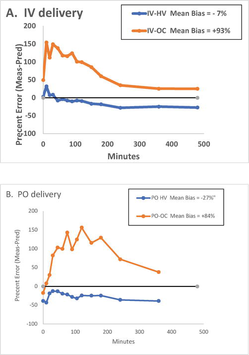
In vivo, cortisol is metabolized to cortisone by the 11-hydroxysteroid hydrogenase 2 (11-HSD2) enzyme expressed in kidney and other tissues. Cortisone binds CBG with intermediate affinity [14], raising the possibility that other metabolites of cortisol might also compete for CBG-cortisol binding. This hypothesis was further explored in an analysis comparing women on oral contraceptive pills (OC) and healthy volunteer (HV) groups based on data of Perogamvros et al. [58, 59]. The data set was especially useful for modeling cortisol distribution in vitro, since multiple measurements of X_TotF, X_F, and free cortisone (X_E) were obtained in the same individual at multiple time points spanning a broad range of cortisol concentrations. Using measured concentrations of X_TotF and X_TotCBG to predict X_F based on Coolens’ formula (represented in Table 2), we compared model-predicted vs. measured concentrations of X_F at each time point. As shown in Figure 1, the residual plots (measured X_F minus X_F estimated using Coolens’ formula) demonstrate the following: (i) Coolens’ formula provides a fair but inconsistent approximation to measured X_F in HV, (ii) in the OC group, X_F predicted by Coolens’ formula significantly underestimates measured concentrations of X_F, with up to 100% percent error in calculated X_F, (iii) the pattern of residual error was time-varying in both groups, but was more prominent in OC, (iv) the pattern of residuals differed for per os (po) and iv modes of hydrocortisone administration, roughly paralleling measured concentrations of X_TotF and X_F. We hypothesized that time-varying concentrations of competitor (P) resulted in higher concentrations of free cortisol than predicted by the Coolens’ formula, which considers cortisol as the sole ligand involved in CBG binding (single row in Table 2).

Figure 1.

Percent error (bias) showing mean residuals (measured minus model-predicted free cortisol concentration) In healthy volunteers (HV, blue) vs. women on oral contraceptives (OC, red) following iv bolus (20 mg) (Panel A) and po hydrocortisone (20 mg) (Panel B). Model-predicted free cortisol concentrations (XF’) were obtained using K11 and N values taken from literature (Coolens’ formula, see Matrix #2). XF estimated by Coolens’ formula significantly underestimated measured XF in women on OC.

In addition, we compared parameter solutions and residual plots for two alternative models. These parameter solutions represent the inverse matrix problem, as discussed also later in Section 6. That is, since X_F and X_TotF were measured at each time point, we used measured concentrations of X_TotF and X_F and assumed constancy of baseline X_TotCBG to iteratively solve for model-specific parameters of interest. In the minimal model, represented by Table 2, these parameters include K₁₁ and N. In the competition model, represented by 2 × 2 Table 5, additional parameters, including affinity constant for competitor (P) binding to CBG [K₂₁], were obtained. Our finding that the competition model provided significantly better fit to experimental data as well as better residual plots compared to the minimal model provide additional support, albeit indirect, for the presence of ligands (P) that compete for CBG-cortisol binding [58]. The identity of the putative ligand(s) (P) remains speculative. However, since endogenous corticosteroid was suppressed in this study by antecedent administration of dexamethasone [59], these observations raise the possibility that other ligands, for example metabolites of cortisol (or progestin in OC), might compete for CBG-cortisol binding. As free cortisone concentrations were also assayed at each time point and its CBG-binding affinity may be taken from the literature [14, 59], we were able to demonstrate that the transient increase in free cortisone concentrations observed after iv and po hydrocortisone bolus was not of sufficient magnitude to account for the observed difference between measured and model-predicted X_F (data not shown). However, it remains possible that other cortisol metabolites may increase in tandem with free cortisone with timing entrained by time-varying concentrations of X_F, the substrate for enzymes of cortisol metabolism. In the hypothetical example of multiple competing ligands, it may be possible to re-parameterize their integrated effects as a composite function represented by a harmonic mean (data not shown).

In summary, there are several validated examples of ligands that compete for CBG-cortisol binding; these include progesterone, adrenal steroid precursors of cortisol biosynthesis, synthetic compounds such as prednisolone, and metabolites of cortisol, such as cortisone.

At equilibrium in the test tube, the concentration of X_F is also affected by albumin-cortisol binding. As shown in Table 2, albumin-cortisol binding may be simplified [3] as a constant ratio (N) of albumin-bound to free cortisol (X_FA/X_F = K₁₂*A). However, whether the simplification of using total (X_TotA) as a surrogate for free albumin (X_A) concentration is appropriate remains uncertain, as discussed in Section 7. Before addressing Coolens’ assumption that X_TotA ≈ X_A, let us first examine some useful data concerning the albumin-cortisol affinity constant (K₁₂). For this purpose we revisit albumin-cortisol binding data previously reported by Lewis et al. [27]. These experiments involve binding of ³H-labeled cortisol to a purified solution of human albumin and will assume 1:1 stoichiometry of albumin-cortisol binding. Consideration of multiple cortisol binding sites per albumin molecule is discussed in Appendix 4.

6. Albumin-cortisol binding in purified solution of human serum albumin using data of Lewis et al.

The experiment involves addition of a small mass of ³H- labeled cortisol (E), which is assumed to bind albumin with an affinity equal to that of endogenous (unlabeled) cortisol (F), to solutions of varying concentrations of purified albumin [27]. Thus, the test tube consists of TotA and TotE, which at equilibrium also gives a free E and a free A. The 1 × 1 matrix for 1 ligand (E) and 1 binding protein (albumin) is shown in Table 7.

Table 7.

1 × 1 matrix for equilibrium equations for experimental cortisol binding studies using purified albumin solution [27].

For these in vitro studies reported by Lewis et al. ³H-cortisol (F) is added to varying concentrations of purified albumin solution [27]. Added ³H-cortisol is distributed between free (measured) and albumin-bound fractions at equilibrium, and here TotF is the amount of ³H-cortisol added to the test tube. F is measured (light red), TotF and TotA are otherwise known (yellow). The affinity constant for albumin-cortisol binding is solved (blue) using varying concentrations of TotA, where the fraction R = F/TotF and, according to (Feldman’s) row eq. 1/R = 1 + ${\mathrm{K}}_{11}$ $·\mathrm{A}$. Applying Coolens’ assumption ${\mathrm{K}}_{11}$ F < < 1 [3], then A = TotA. The plot of 1/R versus experimentally varied TotA provides a series of points which is nearly linear with slope = ${\mathrm{K}}_{11}$. Goodness of fit of this model for the purified albumin assay can be judged by deviations from linearity. Note that this is an inverse problem in that the total and free concentrations are measured or experimentally known and the affinity constant ${\mathrm{K}}_{11}$ is to be estimated.

Constraints: ${\mathrm{K}}_{11}$F < < 1; note that in this experiment, N = ${\mathrm{K}}_{11}A$ =${\mathrm{K}}_{11}\mathit{\text{TotA}}$ and N varies in relation to experimentally varied TotA.

In the albumin-cortisol binding experiments of Lewis et al. [27], concentrations of free and albumin-bound E are measured and, using known values of X_TotA and the measured values of the percent free cortisol (R), the affinity constant (K₁₂) and corresponding equilibrium dissociation constant $K_{12}^{-1}$ is estimated (blue). Conservation of mass laws give

$$\text{TotE}=\mathrm{E}\left(1+K_A\mathrm{A}\right),\text{or}E=\frac{\mathit{\text{TotE}}}{1+K_A\mathrm{A}}.$$E12

Rewriting Eq. (12) in terms of R = fraction that free E is of the total TotE, we have

$$\frac{1}{R}=1+K_A\mathrm{A}.$$E13

The conservation of mass in the column gives

$$\text{TotA}=\mathrm{A}\left(1+K_A\mathrm{E}\right),\text{or}A=\frac{\mathit{\text{TotA}}}{1+K_{A}E}$$E14

to be estimated.

Rewriting (14) in terms of dissociation constant K_D = 1/K_A, we have $A=\frac{{\mathrm{K}}_{\mathrm{D}}\mathit{\text{TotA}}}{{\mathrm{K}}_{\mathrm{D}}+E}$.

Now Coolens’ approximation E < < ${\mathrm{K}}_{\mathrm{D}}$ applies, in which case A = TotA. Then

$K_{A}A=K_A\mathit{\text{TotA}},$ so that Eq. (12) becomes

$$\frac{1}{R}=1+K_A\mathit{\text{TotA}}$$E15

Note that we also use the notation $K_A\mathit{\text{TotA}}=N$ to represent N in Coolens’ formula, which in this formulation indicates that N is proportional to X_TotA.

Assuming 1:1 stoichiometry of albumin-cortisol binding, a graphical estimate of $K_A$ is obtained by plotting 1/R versus TotA and fitting the regression line where the slope is the estimate $K_A$. Data from Lewis et al. [27] are shown in Table 8, R represents the free ³H-cortisol concentration expressed as a fraction of total ³H-cortisol [free ³H-cortisol]/[albumin-bound ³H-cortisol+ free ³H-cortisol].

Table 8.

Data for free cortisol concentrations in binding studies of purified human albumin solution reported by Lewis et al. and associated plot of transformed free cortisol (F) vs. albumin concentration.

A. Data from Lewis et al. purified albumin assay [27]. The experiment involves fixed concentration of labeled cortisol (F) added to solutions of varying concentrations of purified albumin, where the fraction R = free F/TotF. B. Associated plot with slope K₁₁ = 0.0771 per g/L according to eq. 1/R = 1 + ${\mathrm{K}}_{11}$ $·\text{TotA}$, applying Coolens’ assumption ${\mathrm{K}}_{11}$ F < < 1, then A = TotA). The conversion to units nmol/L gives 0.0771/(15,047) = 5.124 × 10⁻⁶ per nmol/L and in terms of dissociation constant K_D = 1/5.124 × 10⁻⁶ = 195,200 nmol/L.

Plotting this data and fitting a regression line gives the graph shown in the plot associated with Table 8, which corresponds to $K_{12}^{-1}$ ≈ 195,000 nmol/L. At median concentrations of serum albumin (580,000 nmol/L), this $K_{12}^{-1}$ ≈ 195,000 nmol/L corresponds to N = 3.0. Lewis et al. addressed the issue of discrepant values for N in purified albumin solution (3.0) vs. the lower N (1.74) for plasma/serum samples used in Coolens’ quadratic equation human serum [27]. They note that “in physiological human albumin solutions 25% of ³H-cortisol is in the free fraction…This may suggest that the ratio of albumin-bound to unbound cortisol is 3.0, which is slightly higher than the value of 1.74 value used in the Coolens’ calculation of free cortisol from total cortisol and CBG. Taken together we suggest that revision of the Coolens’ value is probably not warranted” [27].

7. Toward a general theorem that includes competition for albumin-cortisol binding (2 × 2 matrix)

7.1 Coolens’ simplification (re-parameterization of albumin-bound cortisol)

Coolens’ assumption re-parameterizes the equation used to estimate the concentration of albumin-bound cortisol, which is represented by the inner cell indicated by dashed oval in Table 1. In the cubic solution, the mass action equation for albumin-bound cortisol (FA) is the product of K₁₂*F*A, where K₁₂ is the equilibrium affinity constant for albumin-cortisol binding, F is the concentration of free cortisol, and A is the concentration of free albumin. Coolens’ simplification of this equation transitions K₁₂*A to a single value (N). N is a constant, which makes the implicit assumption that both K₁₂ and A are also constant. A related assumption is that $\mathrm{F}<<K_{12}^{-1}$, which implies that $\mathrm{F}/K_{12}^{-1}$ is a very small number. In a simplified model that only considers one ligand (cortisol), these assumptions suggest that TotA = free A and that free A is unaffected by changes in F within the physiologic range of systemic cortisol concentrations.

To visualize the re-parameterization of albumin-bound cortisol in the matrix format, we refer to Table 1 and focus on the column sum (compound box) showing that $\mathit{\text{TotA}}=A\left(1+K_{12}F\right)$. Given Coolens’ assumption that $\mathrm{F}<<K_{12}^{-1}$ and dividing through by $K_{12}^{-1}$, we obtain $K_{12}·F<<1$, so that in the column sum $\mathit{\text{TotA}}=A\left(1+K_{12}F\right)\cong A\left(1+0\right)=\mathrm{A}$, which is a constant (TotA). Now $K_{12}A\cong K_{12}\mathit{\text{TotA}}=N$ is a constant. So we can replace $K_{12}\mathit{FA}\text{in the matrix}\mathrm{by}\mathit{NF}$, as shown in Table 2.

Coolens’ Theorem. In the 1 × 2 matrix above, if $K_{12}F<<1$, then

1. $\frac{\left[\mathit{FA}\right]}{\left[F\right]}=N\mathit{\text{is}}a\mathit{\text{constant}}$,

2. A is a constant and $K_{12}A=N$,

3. $A\cong \mathit{\text{TotA}}$.

Comment. It is clear that the above theorem is intended for dynamic situations such as occur in vivo in human physiology. For example, statement (i) above means $\frac{\left[\mathit{FA}\right]}{\left[F\right]}$ is constant, as F (and FA) vary over time. Yet, the matrix above describes equilibrium situations such as occur in vitro (in a test tube) or as in a steady state condition in a dynamic system. The connection is often that the equilibrium in vitro is a representative (snapshot) in time of the dynamic process. In equilibrium in a test tube, dynamic variables become constants, as discussed in Section 1 above. This view might be considered accurate even in vivo, because binding takes place so quickly in time while other time-varying processes in the in vivo dynamic system develop relatively much more slowly.

Condition iii) is not absolutely necessary. See the general theorem below.

To introduce the general theorem, we consider Coolens’ assumptions and Coolens’ simplification to the context of competitive protein-ligand binding reactions where multiple ligands may compete with cortisol for albumin binding at one (or more) binding sites. These considerations may be generally applicable to BP’s associated with non-specific binding reactions in which many ligands (multiple rows in nxm matrix) may be involved. As well, the theorem generally applies to BPs having high molar concentration in serum relative to molar concentration of the ligand(s) of interest. Because the concentrations of BPs, ligands, and competing ligands are constant in the test tube, the assumption of constancy of N as a means of simplifying numerical solutions for X_F may be most realistic in vitro. As addressed below, N may vary under different conditions that affect the ratio of X_FA/X_Fin vivo, including supernumerary binding reactions that influence the concentration of free albumin (X_A) as a percent of total (X_TotA).

7.2 Theorem for generalization of Coolens’ N

Without pre-condition and in all matrices and for every ligand P with the concentration [PA] and assuming 1:1 stoichiometric ligand P-albumin binding, we have

1. $\frac{\left[\mathit{PA}\right]}{P}=N_P$ is a constant if and only if

2. A is a constant and then $N_P=K_{P}A$ and $N_P$ is constant.

3. If A is constant then all mass action equations for A in the general matrix can be replaced by $N_{P}P$ for every ligand P.

Proof. By the mass action equation for cortisol-albumin binding $\frac{\left[\mathit{PA}\right]}{\left[P\right]}=K_{P}A$, so defining $N_P=\frac{\left[\mathit{PA}\right]}{\left[P\right]}$, we have $N_P$ is constant if and only if A is constant.

For example, without loss of generality, considering 2 × 2 matrix where ligand P is a competitor to F in binding to A, we obtain the matrix shown in Table 5.

Writing $\mathit{\text{TotA}}=A\left(1+K_{12}F+K_{22}P\right)$, a generalization of Coolen’s condition might be $K_{12}F+K_{22}P\ll 1,\mathit{\text{in which case}}A\cong \mathit{\text{TotA}}$ is a constant. By the general theorem above, both $K_{12}A=N_F\mathit{\text{and}}{K}_{22}P=N_P$ are constants. In the 2 × 2 matrix above the mass action equations for A can be replaced by $N_{F}F$ and $N_{P}P$ as shown by iii) in the general theorem. The resulting 2 × 2 matrix is shown in Table 9.

Table 9.

2 × 2 matrix for cortisol binding equilibrium equations with Coolens’ approximation.

The three total concentrations: total cortisol (TotF), total competitor (TotP), and total CBG (TotC) are measured (light red). The affinity constants for CBG-cortisol (K₁₁) and albumin-cortisol (K₁₂) binding are obtained from the literature or otherwise estimated (yellow). Assuming P is a specific ligand, the Coolens constants for ligand-albumin binding (N₂₁) and (N₂₂) may be obtained from the literature (yellow). The free cortisol and free competitor concentrations (F and P) are estimated (light blue).

Constraints: General Coolens’ assumption, $K_{12}F+K_{22}P\ll 1.$

To take advantage of this simplification, this 2 × 2 matrix can be collapsed into a 2 × 1 matrix, which is useful for computation purposes, as shown in Table 10.

Table 10.

2 × 1 matrix simplification by application of general Coolens’ assumption.

By algebraic manipulation, one column from the 2 × 2 matrix (Table 9) can be combined with the marginal column of free concentrations; thus, one column from Table 9 is eliminated, resulting in Table 10, a 2 × 1 matrix.

Constraints: General Coolens’ assumption, $K_{12}F+K_{22}P\ll 1.$

There is one more step that could be taken to explain that this equilibrium solution results in a cubic equation in terms of free C. Then using the solution for C, the Feldman equations result in solutions for free F and free P. That step is to use the Duality Theorem mentioned after the general equilibrium n × m matrix in Table 6, which transposes rows and columns. Thus, the 2 × 1 matrix (Table 10) becomes a 1 × 2 matrix, shown in Table 11, and the characteristic polynomial is of degree m + 1 = 2 + 1 = 3, a cubic equation in C. Once the value of C is obtained, the Feldman Eq. (12) give solutions for free F and free P (see caption of Table 11).

Table 11.

1 × 2 matrix, the transpose of 2 × 1 matrix in Table 10, for cortisol binding equilibrium equations with Coolens’ approximation.

This table illustrates the application of the Duality Theorem to change the 2 × 1 matrix (Table 10) into an equivalent 1 × 2 matrix (Table 11). Using this transformation, equilibrium equations can be solved first for free CBG concentration (C).

The conservation of mass equations are:

$$\begin{array}{l}\mathit{\text{TotC}}=C\left(1+K_{11}F+K_{21}P\right)\\ \mathit{\text{TotF}}=F\left(1+N_{12}+K_{11}C\right)\mathit{\text{or}}F=\mathit{\text{TotF}}/\left(1+N_{12}+K_{11}C\right)\\ \mathit{\text{TotP}}=P\left(1+N_{22}+K_{21}C\right)\mathit{\text{or}}P=\mathit{\text{TotP}}/\left(1+N_{22}+K_{21}C.\right)\end{array}$$

Now substituting F and P formulae into the first equation and clearing fractions gives a cubic Eq. (6) in C with all coefficients known.

Finally, this value of C can be substituted into the Feldman Eq. (12) for F and P above gives the values for free F and free P.

Constraints: General Coolens’ assumption, $K_{12}F+K_{22}P\ll 1.$

Corollary 1. In the 2 × 2 matrix above, if $K_{12}F\ll 1$ and P is constant then the following are true and equivalent:

1. $\frac{\left[\mathit{PA}\right]}{P}=N_P$ is a constant if and only if

2. A is a constant and $K_{P}A=N_P$,

3. If A is constant then all mass action equations for A in the matrix can be replaced by $N_{P}P$ for every ligand P including F.

Proof. Write $\mathit{\text{TotA}}=A\left(1+K_{12}F+K_{22}P\right)=A\left(1+0+K_{22}P\right)$, so that

A is constant if and only if P is constant and the rest is true by the general theorem.

Comment 1. In general, if any $N_P=K_{P}A$ were not constant then A is not constant and then no other $N_P$ is constant. These are an all-or-none result; every K_A in the A column can be replaced by constants $N_P$ (they may be different constants) or none of them can be replaced by constants $N_P$.

Comment 2. In Corollary 1, for the 2 × 2 matrix, the fact that N is constant requires A to be constant, which if A < TotA requires P to be constant seems to be difficult to realize in vivo, but not in vitro.

Another problem may occur when A < TotA in that we may no longer know the value of $N_P=K_{P}A$.

Let us summarize comment 1 as corollary 2.

Corollary 2. In the general matrix, if any $N_P=K_{P}A$ were constant then all the other $N_P$ are constants; and in vivo, if any $N_P=K_{P}A$ were not constant then all the other $N_P$ are not constants.

Proof. Any $N_P=K_{P}A$ is constant if and only if A is constant, and A is constant if and only if all $N_P=K_{P}A$ are constant.

Corollary 3. In the 2 × 2 matrix above, if $K_{12}F\ll 1$ and $K_{22}P\ll 1$ then the following are true:

1. A = TotA

2. $\frac{\left[\mathit{PA}\right]}{P}=N_P$ and $\frac{\left[\mathit{FA}\right]}{F}=N_F$ are constant and

3. $N_P=K_P\mathit{\text{TotA}}$ and $N_F=K_F\mathit{\text{TotA}}$ .

Proof. Write $\mathit{\text{TotA}}=A\left(1+K_{12}F+K_{22}P\right)$. Then $\mathit{\text{TotA}}=A\left(1+0+0\right)=A$,

Comment 3. In the above general theorem, we considered competition as one competitor, P. However, one may think of this P as a composite of many competitors P. A more formal analysis of this could be done using multiple competitors P as multiple additional rows in our matrix.

7.3 What if there are multiple cortisol binding sites on the albumin molecule?

The albumin-cortisol binding reaction is often simplified by assumption of (1:1) stoichiometry, whereby one molecule of albumin binds one molecule of cortisol. However, it is possible that albumin has more than one binding site for cortisol, as has been suggested for albumin binding of testosterone for example [60]. The matrix approach can still be usefully applied in the example of multiple binding sites, though care must be taken to distinguish ‘per site’ vs. ‘per molecule’ binding activities in the matrix. This is especially critical when dealing with conservation of mass equations for albumin in the multiple binding site model since an important operational objective of the matrix is to relate marginal totals to measured data. In the case of albumin, measured data is reported in molecular mass (g/L or mmol/L) rather than theoretical number of binding sites. A matrix approach to multiple cortisol binding sites on the albumin molecule is described in Appendix 4.

7.4 Current perspectives on albumin-cortisol binding

Competition probably affects albumin-cortisol binding and equilibrium concentrations of albumin-bound cortisol in vitro. The competitors having the greatest potential impact on free cortisol concentrations are ones that circulate at high concentrations and bind albumin with significant affinity, such as free fatty acids [60]. Our general theorem represented in Table 9 suggests that the simplification for albumin-bound cortisol using a constant (N) is applicable if N can be reasonably estimated. A key element in this objective is ascertainment of free albumin (X_A) as a percent of total albumin (X_TotA). By the same token, there is evidence that free A varies in relation to total A. Thus, it appears that free albumin concentrations (X_A), and consequently values for N, are reduced in hypoalbuminemic subjects [29, 61].

Given ease of measurement of serum total albumin concentrations, it may be useful to adjust N based on measured concentrations of X_TotA. On the other hand, the impact of variation in N on free cortisol concentration is relatively small under conditions where most of the hormone is bound by CBG. Thus, in some formulations, such as Coolens’ quadratic equation, normative rather than measured values for X_TotA are applied with minimal impact of free cortisol estimates; similar assumptions of normative values for X_TotA and N are made in formula used to estimate free testosterone and vitamin D concentrations [62, 63]. However, for conditions such as critical illness, septic shock, or CBG-deficiency in which bioavailable cortisol ((X_F + X_FA) = F(1 + N)) represents a more substantial fraction of X_TotF, error associated with selection of an incorrect value for N has a more significant impact on estimated X_F. Given these uncertainties concerning both the constancy and value for N, additional investigations concerning the use of Coolens’ simplification to model albumin-bound cortisol concentrations are warranted.

8. Conclusions

We have introduced a matrix format for equilibrium (1) as a guide to writing down the Feldman equations, (2) to represent a given equilibrium problem/discussion in vitro or in vivo marking what is known and what is to be computed, (3) as an illustration of several formulations given in the literature, and (4) as an aid to computations/simplifications, as illustrated by Appendix 4. Although the present chapter has focused on cortisol, it may be understood that the matrix approach described herein is generalizable to analogous problems, including other corticosteroids of interest, sex steroids, thyroid hormones, vitamin D metabolites, and insulin-like growth factor 1. The approach is also generalizable to other ligand-protein binding problems, including substrate-enzyme and antigen-antibody reactions.

The topics treated with this matrix format include:

1. Summary of contemporary models that consider cortisol as the sole ligand involved in BP interactions. A single ligand (cortisol) in nxm matrix yields analytic solutions using cubic (1 × 2), quartic (1 × 3), and quadratic (1 × 2 with re-parameterization of albumin-bound cortisol) equations.

2. Competition model for specific binding, by which multiple ligands compete for the specific serum transport BP (CBG in this case) characterized by high-affinity binding and limiting concentrations. In this example of specific binding, free CBG concentrations vary widely over the physiologic range of (free) cortisol concentrations. This results in saturable kinetics of CBG-cortisol binding. Other ligands may also compete with cortisol for limiting concentrations of free CBG. The competition model is represented by 2 × 2 matrix, which may be generalized to multiple ligands interacting with multiple BPs. Clinical examples of competition for CBG-cortisol binding, including analysis of women on OCP, were also developed using matrix notation. The coupled polynomial equations associated with the 2 × 2 matrix are not tractable to analytic solutions; rather, they require iterative solutions.

3. Competition model for non-specific binding, as exemplified by albumin-cortisol binding. In this situation, the equilibrium dissociation constant for albumin-cortisol binding ($K_{12}^{-1})$greatly exceeds the concentration of free cortisol ($K_{12}^{-1}>>{\mathrm{X}}_{\mathrm{F}}$); consequently, the free concentration of albumin (A) varies insignificantly over the physiologic range of free cortisol concentrations. The albumin-cortisol binding reaction was first addressed using a 1 × 1 matrix to represent the in vitro³H-cortisol binding experiments reported by Lewis et al. using purified albumin solutions [27].

4. The matrix for non-specific binding was subsequently expanded to a general, competitive (2 × 2) model and theorem for Coolens’ simplification, which considers albumin-bound cortisol (X_FC) as a constant ratio (N) of albumin-bound to free cortisol concentrations. The generalized theorem raises the possibility that, given the multiplicity of ligands that bind albumin, the concentration of free albumin (A) may be less than total albumin concentration (A < TotA).

5. CBG binds cortisol with 1:1 stoichiometry, but there is a possibility of complex stoichiometry in the case of albumin-cortisol binding. Development of per site and per molecule matrix notation was useful for modeling the hypothetical example of multiple, independent cortisol-binding sites per albumin molecule. This approach was useful for multiple sites having different affinity constants for albumin-cortisol binding. However, in order to fulfill the objective of relating the matrix totals to measured totals (e.g., total albumin concentration in serum), it is important to account for sites per molecule when applying mass conservation equations.

The recognition that ligands other than cortisol that influence CBG-cortisol binding reactions closes a chapter on simple polynomial equations that consider cortisol as the sole binding ligand. The generalized system of Feldman equations, represented by the 2 × 2 matrix, involves coupled polynomial equations. In the presence of other competing ligands (P), estimation of free cortisol involves iterative rather than simple analytic solutions. In the case of albumin-cortisol binding, the multiplicity of ligands involved in non-specific binding challenge the assumption that free albumin is equal to total albumin and complicate accurate assessment of N. Thus, while N may be constant in vitro, N may vary between individuals and vary over time and condition within an individual subject. If N is not a constant and might vary within and between individual subjects, the simplicity of a constant N is no longer applicable. In that case, alternative measures to predict albumin-bound cortisol concentration or estimate N may be needed to accurately solve free cortisol concentrations. Since X_TotA is simply and routinely measured clinical laboratory, the challenge becomes determination of free albumin as a percent of X_TotA. With these (X_TotA and X_A) in hand, there may be an approach to solving for affinities or Coolens’ N. Accurate assessment of N is more important in conditions, such as critical illness or exogenous hydrocortisone administration, where bioavailable cortisol represents a more substantial percentage of total cortisol.

In summary, the principles of mass action and conservation continue to govern the distribution of cortisol between free and protein-bound compartments in vitro. Alternative modeling approaches (and/or alternative measurements) may be needed to resolve the clinical problem of accurately estimating X_F without having to use laborious separation methods. We hope that this chapter provides a way forward on this important task.

Acknowledgments

The authors thank Frank K. Urban III, Professor of Electrical & Computer Engineering at Florida International University, Miami, FL for helpful discussion of the material. The research was supported by the Research Service of the New Mexico Veterans Administration Healthcare System in Albuquerque, NM. We wish to acknowledge Ilias Perogamvros, David Ray, Brian Keevil, Leon Aarons, Adrian Miller, and Peter Trainer at University of Manchester, UK, who generously provided the cortisol concentration data used in Figure 1 and related modeling analysis [2, 58, 59].

Conflict of interest

The authors declare no conflict of interest.

Appendices

Appendix 1. A connection between dynamic model in vitro and equilibrium solutions in vitro:

The CBG-cortisol binding reaction in our four compartment model of in vivo cortisol distribution (2) applied to the in vitro experiment is represented by the differential equation $\frac{\mathit{dFC}\left(t\right)}{\mathit{dt}}=-{\kappa }_{-1}F\left(t\right)C\left(t\right)+{\kappa }_{1}C\left(t\right)F\left(t\right)$, where F is the free cortisol, C is the free CBG, and FC is CBG-bound cortisol; ${\kappa }_1$and ${\kappa }_{-1}$ are the on and off rates of this cortisol-CBG reaction. Rewriting this differential equation in a standard form: $\frac{\mathit{dFC}}{\mathit{dt}}+{\kappa }_{-1}\mathit{FC}={\kappa }_{1}C·F$, there is a well-known integral solution, and we get a convolution integral solution:

$\mathrm{FC}\left(\mathrm{t}\right)=\frac{{\kappa }_1}{{\kappa }_{-1}}{\int }_0^t{\kappa }_{-1}exp\left(-{\kappa }_{-1}\left(\mathrm{t}-\mathrm{\tau }\right)\right)C\left(\tau \right)F\left(\tau \right)d\mathrm{\tau }$, provided we start at $\mathrm{FC}\left(0\right)=0.$

We recognize that the dynamic reaction of F binding to CBG to form the bound FC is proportional to a delayed version of the function C × F according to convolution integral solution. The half-life of the reaction = $\frac{\mathit{ln}2}{{\kappa }_{-1}}$ which equals $\frac{.69}{.88/\mathit{sec}}=0.8\mathit{\text{seconds}}$ for typically reported values of this off rate. The constant of proportionality is $\frac{{\kappa }_1}{{\kappa }_{-1}}=\frac{.027/\mathit{nM}-\mathit{sec}}{.88/\mathit{sec}}=.03/\mathit{nM}$, which engineers might call gain and biochemists call the affinity or association constant of the reaction; the reciprocal =33 nM is the disassociation constant. We also recognize that FC, C, and F are constants at equilibrium, and that $\frac{\mathit{dFC}}{\mathit{dt}}=0$implies FC = K₁₁ CxF, which is the mass action equation for this reaction and is used in the equilibrium solution in vitro.

Next as an illustration of a general result, we show that the steady state solutions of the differential equations governing the dynamic behavior of three compartments (free, CBG-bound and albumin-bound cortisol) in vitro, in the test tube, are the same as the solutions of Feldman’s iterative equations for that same test tube. The introductory sections entitled “Free, CBG-bound, and albumin-bound cortisol as a 3-compartment model” and “Cortisol in captivity” in the manuscript describe the in vitro situation represented in a test tube. The system of three differential equations for this 3-compartment model are

$$\begin{array}{l}\frac{\mathit{dF}\left(t\right)}{\mathit{dt}}=+{\kappa }_{-1}^C\ast \mathit{FC}\left(t\right)-{\kappa }_1^{C}C\left(t\right)\ast F\left(t\right)+{\kappa }_{-1}^A\ast \mathit{FA}\left(t\right)-{\kappa }_1^{A}A\left(t\right)\ast F\left(t\right)\\ \frac{\mathit{dFC}\left(t\right)}{\mathit{dt}}=-{\kappa }_{-1}^C\ast \mathit{FC}\left(t\right)+{\kappa }_1^{C}C\left(t\right)\ast F\left(t\right)\\ \frac{\mathit{dFA}\left(t\right)}{\mathit{dt}}=-{\kappa }_{-1}^A\ast \mathit{FA}\left(t\right)+{\kappa }_1^{A}A\left(t\right)\ast F\left(t\right)\end{array}$$E16

where $C\left(t\right)=\mathit{\text{TotCBG}}-\mathit{FC}\left(t\right)\text{and}A\left(t\right)=\mathit{\text{TotA}}-\mathit{FA}\left(t\right).$

The steady state solutions are these limits: $\underset{t\to \infty }{lim}F\left(t\right)=F\left(\infty \right),$

$\underset{t\to \infty }{lim}\mathit{FC}\left(t\right)=\mathit{FC}\left(\infty \right),\mathit{\text{and}}\underset{t\to \infty }{lim}\mathit{FA}\left(t\right)=\mathit{FA}\left(\infty \right),$ The where clause in Eq. (4) in this chapter also implies the limits $\underset{t\to \infty }{lim}C\left(t\right)=C\left(\infty \right),\mathit{\text{and}}\underset{t\to \infty }{lim}A\left(t\right)=A\left(\infty \right)$ exist.

On the other hand, the Feldman iterative equations are derived by schoolbook algebra from the conservation of mass and mass action system of equations

$$\begin{array}{l}\mathit{Tot}F=F\left(1+K_{11}C+K_{12}A\right),\\ \mathit{Tot}C=C\left(1+K_{11}F\right)\\ \mathit{Tot}A=A\left(1+K_{12}F\right)\end{array}$$E17

The question is are iterative solutions for the equilibrium (F, C. and A) the same as the steady state solutions $F\left(\infty \right)$, $C\left(\infty \right),\mathit{\text{and}}A\left(\infty \right)?$

We proceed using the convolution solution obtained above for FC(t); thus under technical conditions satisfied here, we obtain

$$\begin{array}{lll}\mathrm{FC}\left(\infty \right)& =& \underset{t\to \infty }{lim}\mathit{FC}\left(t\right)=\underset{t\to \infty }{lim}{K}_{11}{\int }_0^t{\kappa }_{-1}exp\left(-{\kappa }_{-1}\left(\mathrm{t}-\mathrm{\tau }\right)\right)C\left(\mathrm{\tau }\right)F\left(t\right)d\mathrm{\tau }\\ & =& K_{11}C\left(\infty \right)F\left(\infty \right)\underset{t\to \infty }{lim}{\int }_0^t{\kappa }_{-1}exp\left(-{\kappa }_{-1}\left(\mathrm{t}-\mathrm{\tau }\right)\right)d\mathrm{\tau }\end{array}$$

where ${\left.{\int }_0^t{\kappa }_{-1}exp\left(-{\kappa }_{-1}\left(\mathrm{t}-\mathrm{\tau }\right)\right)d\mathrm{\tau }=exp\left(-{\kappa }_{-1}\left(\mathrm{t}-\mathrm{\tau }\right)\right)\right|}_0^t=1-e^{-{\kappa }_{-1}t}$

and $\underset{t\to \infty }{lim}\left\{1-e^{-{\kappa }_{-1}t}\right\}=1.$ Thus, the steady state solutions satisfy the mass action eq. $\mathrm{FC}\left(\infty \right)=K_{11}C\left(\infty \right)F\left(\infty \right).$ It is clear that the third equation of Eq. (16) results in a convolution solution for FA(t) and that the steady state solutions satisfy the mass action eq. $\mathrm{FA}\left(\infty \right)=K_{11}A\left(\infty \right)F\left(\infty \right).$

It is now convenient to sum the 3 equations in the system of Eq. (16) to obtain

$$\frac{d\left(F\left(t\right)+\mathit{FC}\left(t\right)+\mathit{FA}\left(t\right)\right)}{\mathit{dt}}=0\mathit{\text{for}}\mathit{all}t\ge 0.$$

This implies F(t) + FC(t) + FA(t) = a constant for all t and we recognize that the constant is TotF. Taking the limit as $t\to \infty$ gives that the steady state solutions satisfy the conservation of mass equation $F\left(\infty \right)+\mathit{FC}\left(\infty \right)+\mathit{FA}\left(\infty \right)=\text{TotF}$.

All this information implies that that the steady state solutions also satisfy the second and third equations of Eq. (16) above and the corresponding Feldman iteration equations and Feldman equilibrium solutions are the same as the steady state solutions.

Comment. The usual method of setting derivatives equal zero to obtain steady state solutions works here and works more quickly, but the above proof gives steady state solutions directly as limits, which is instructive.

Appendix 2. Descartes’ Rule of Signs and existence and uniqueness of iterative solutions

Cartesian side bar: Descartes’ Rule of Signs was published in 1637 by Rene Descartes in his work La Geometrie. The rule states that if the non-zero terms of a single-variable polynomial with real coefficients are ordered by descending variable exponent then the number of positive roots of the polynomial is either equal to the number of sign changes between consecutive (non-zero) coefficients or is less than it by an even number. A root of multiplicity k is counted as k roots. A corollary is that the number of negative roots is the number of sign changes after multiplying the coefficients of odd power terms by −1, or fewer than it by an even number. In 1828, Carl Friedrich Gauss improved the rule by providing the proof that when there are fewer roots of polynomials than there are variations of sign, the difference between the two is even.

End of side bar.

We have shown existence of positive solutions for each of the coupled characteristic polynomials by our Existence Theorem. We need to connect this with the iterative solutions and note that these solutions can exist simultaneously so that we have vector solutions for $\mathrm{P}=\left(P_1,\cdots ,P_n\right).$

Let vector P^ν be the iterations of Eq. (8) and Q^ν be the iterations of Eq. (9). Suppose that the limits $\underset{\nu \to \infty }{lim}{\mathrm{P}}^{\nu }=P$ and $\underset{\nu \to \infty }{lim}{\mathrm{Q}}^{\nu }=Q\text{exist}.$Writing Feldman’s iterative equations as the functions ${\mathrm{P}}^{\nu }=\mathrm{f}\left({\mathrm{Q}}^{\mathrm{\nu }}\right)\text{and}{\mathrm{Q}}^{\mathrm{\nu }}=\mathrm{g}\left({\mathrm{P}}^{\nu -1}\right)$, the composition is ${\mathrm{P}}^{\nu }=\mathrm{f}\circ \mathrm{g}\left({\mathrm{P}}^{\nu -1}\right)$ and taking limits we obtain $\mathrm{P}=\mathrm{f}\circ \mathrm{g}\left(\mathrm{P}\right)$, since f, g and $\mathrm{f}\circ \mathrm{g}$ are continuous functions. This last equation can be solved for P as a system of coupled polynomial equations. Coupled refers to the fact the coefficients of the polynomial in P_i depend on the other P_k, k ≠ i. This shows the iterative solutions are the same as the polynomial roots. Note that the commonly used term “root” of a polynomial is a solution of the polynomial set equal to zero.

If we are concerned the limits P and Q may not exist, then we note that each $P_i$ satisfies the inequalities, $0\le P_i\le \mathrm{Tot}{P}_i$ for i = 1, …, n, which is a closed (compact) box and the Heine-Borel theorem guarantees at least one limit point P in this box and a subsequence of ${\mathrm{P}}^{\nu }$’s converging to this P. The same argument as above guarantees that this P satisfies our system of coupled polynomials. In fact, for every limit point this is true. If all the limit points were equal, then the limit exists and is unique. Thus, the uniqueness of the iterative solutions is related to the uniqueness of the polynomial positive roots. So, the only question remaining is: Does the system of polynomial equations have one and only one positive solution? Negative and imaginary solutions of the polynomials are extraneous and not possible limits.

Comment. The existence and uniqueness of solutions of Feldman’s iterative equations does not require that we obtain analytic solutions, that is, closed form formula. In fact, analytic solutions are readily available for the roots of polynomials of degree 4 or less, but it has been shown that the general 5th degree polynomials do not have analytic solutions. Most think solutions should be obtained by iterative numerical methods (or perhaps using differential equations). Fortunately, showing existence and uniqueness of solutions does not require analytic solutions.

It is possible to show uniqueness for all nx1 matrices. Each m + 1 degree polynomial is quadratic whose coefficients are in the pattern ($+,0,-$) that has precisely one sign change, and Descartes’ Rule of Signs says the number of positive roots is one or less by 2 or more. Since having less is not possible, there is exactly one positive root, which is uniqueness. The duality of the iterative equations shows uniqueness for all 1 × m matrices.

Summary. We have now shown that the Feldman iterative solutions are the same as the positive root(s) of the characteristic polynomial(s) and that Feldman iterative solutions are also the same as the steady state solutions of the corresponding differential equations (Appendix 1). We have three separate methods for computing equilibrium values in vitro; and we have established existence and uniqueness of these solutions.

Appendix 3. Degree of characteristic polynomials and singular value decomposition

The degree (m + 1) of the polynomial (see Section 4) has been related to the number of binding proteins (Q_j); however, we can reverse the roles of ligands and BPs and obtain (n + 1) degree polynomial. This points out a slight inaccuracy in the presentation above; the truth relates to the number of K_ii > 0, which is related to r equals rank of the matrix K (r = rank(K)).

Let us fix the inaccurate discussion above about the degree of the limiting polynomial; is it (m + 1), (n + 1), or (r = rank(K))? Since the rank of K must be less than or equal to min (m,n) and often is less, the number of positive K_ii’s may be less than (m + 1) and (n + 1). We note that the factors of the limiting polynomial for P_i involve the K_iν’s in the i^th row of K. For the product of linear factors ${\prod }_{\nu \ne i}\left\{K_{\mathit{i\nu }}{P}_i+C_{\mathit{i\nu }}\right\}$, if $K_{\mathit{i\nu }}=0,$then this term becomes a positive constant, and the degree of the polynomial is reduced by one. This is true for every $K_{\mathit{i\nu }}=0$ the i^th row of K. The result is that the degree of characteristic polynomial in $P_i$equals 1 + number of positive K_iν in the i^th row of K.

For another view of the degree of the characteristic polynomial (in a different space), we will use a matrix version of the Feldman equations and the singular value decomposition of the matrix K. This decomposition says every nxm matrix K can be factored as $K=Q_1\sum Q_2^T$ where $\mathit{nxn}\mathit{\text{matrix}}{Q}_1\mathit{\text{and}}\mathit{mxm}\mathit{\text{matrix}}{Q}_2$are each orthonormal ($Q_1^T{Q}_1=I_n$where $I_n=\mathit{nxn}\mathit{\text{identity matrix}}{I}_n$and

$Q_2^T{Q}_2=I_m)$; and where there are r (= rank(K)) positive singular values ${\mu }_i$ which form the diagonal of $\sum$ such that $\sum =\left(\begin{array}{cc}\mathit{diag}\left(\mu \right)& 0\\ 0& 0\end{array}\right)$. Another way of saying this is $K={\sum }_{i=1}^r{\mu }_i{p}_i{q}_i^T$ where $p_i$ ia a left singular nx1 vector corresponding to ${\mu }_i$ (column of $Q_1)$ and $q_i$ is a right singular mx1 vector corresponding to ${\mu }_i$ (column of $Q_2)$.

We may need another matrix theory development for Feldman equations. In addition to matrix algebra, we will need the Hadamard (alternatively called Schur) product of two matrices of the same size defined as by elementwise products; that is, $A\odot B=\left[A_{\mathit{ij}}·B_{\mathit{ij}}\right].$ Note that Hadamard products are commutative: $A\odot B=B\odot A$; whereas the usual matrix product of square matrices is not generally commutative. The Hadamard (Schur) product of two vectors of the same size is similarly defined as $\lambda \odot v=\left[{\lambda }_j·v_j\right]$. The Schur product of a vector and a matrix follows quickly. We should also define Schur division of vectors $\lambda \oslash v=\left[{\lambda }_j/v_j\right]$provided $v_j\ne 0.$The Schur product of vectors can be realized in the matrix algebra using square diagonal matrices like diag (v) whose diagonal is made up of the elements of the vector v and off diagonal entries are all zero: $\lambda \odot v=\mathit{diag}\left(v\right)\lambda =\mathit{diag}\left(\lambda \right)v$ . Also, diag(v)$1=v,$where 1 is a vector with entries all equal to 1. Conversely, diag (v) can be realized using a Schur product: $\mathit{diag}\left(v\right)=v\odot I=I\odot v,$where $I$ is the usual matrix identity.

Comment. The important part of the Feldman equations in terms of matrix theory involves $diag\left(\mathrm{P}\right)\mathrm{K}diag\left(\mathrm{Q}\right)=\left[K_{\mathit{ij}}{P}_i{Q}_j\right].$

The pre-multiplication by diag(P) can be represented by $P\odot K$, but the post-multiplication by diag(Q) operates on the columns of K and is not easily represented by the Schur product $\odot$ since the candidate expression of $K\odot Q$ operates on rows by commutativity and not on columns as required. Attempts at two other expressions give K diag(Q) = K (Q$\odot I)$. This requires a distributive law for computations, which is said not to exist; or alternatively K diag(Q) =${\left(\mathrm{Q}\odot K^T\right)}^T,$ which is also difficult to use in computations.

Feldman Eqs. (1) and (2) with the n × m matrix K, n × 1 vector $=\left[P_i\right]$, and m × 1 vector $Q=\left[Q_j\right]$ can be written as

$$\mathit{diag}\left(P\right)\left\{1_n+K\mathit{diag}\left(Q\right)1_m\right\}=\left[{\mathit{\text{TotP}}}_i\right]$$E18

and

$$\mathit{diag}\left(Q\right)\left\{1_m+K^T\mathit{diag}\left(P\right)1_n\right\}=\left[{\mathit{\text{TotQ}}}_j\right].$$E19

These equations look simpler in a vector form than in the matrix form.

$$\mathrm{P}+\left(P\odot K\right)Q=\mathit{\text{TotP}}$$E20

$$\mathrm{Q}+\left(Q\odot K^T\right)P=\mathit{\text{TotQ}}$$E21

But looks are deceiving. In future work, it may be possible to use matrix algebra augmented by Schur multiplication.

Appendix 4. Matrix application to hypothetical example of multiple cortisol binding sites per albumin molecule: reconciliation of mass conservation per site and per molecule with measured concentrations of total albumin.

Rather than assume simple 1:1 stoichiometry for albumin-cortisol binding, let us consider the more complex, hypothetical scenario where there are three independent cortisol-binding sites per albumin molecule. The per site equilibrium can be also analyzed using the proposed matrix notation. We parse the problem by first discussing per site equilibrium; once the per site equilibrium has been developed, we secondarily discuss per molecule equilibrium. The per site equilibrium is useful to determine the concentration of albumin-bound cortisol using mass action equations, while the per molecule equilibrium is also necessary for conservation of mass equations and relating the solution to clinical measurements in units of mass/volume (of total albumin). In this hypothetical example, let us suppose TotA is the concentration of albumin molecules and the 3 cortisol-binding sites per molecule are numbered 1,2, and 3. Let each site have its own association (affinity) constant, K₁₁, K₁₂, K₁₃, respectively. Let total and free concentration per site be TotA_i and A_i, respectively. Relating concentrations to the number of molecules (or site #1) per unit volume justifies the concept of per site concentration. Note that each TotA_i = A_i. Considering one ligand for this discussion, the 1 × 4 per site matrix can be drawn as (Table A1).

Matrix 1 × 4 per site	C=CBG	$A_1$	$A_2$	$A_3$
$F$	$K_{1}C\bullet F$	$K_{11}{A}_1\bullet F$	$K_{12}{A}_2\bullet F$	$K_{13}{A}_3\bullet F$	$\mathit{\text{TotF}}$
	TotC	$\mathit{\text{TotA}}$	$\mathit{\text{TotA}}$	$\mathit{\text{TotA}}$

Table A1.

1 × 4 matrix per site for 3 independent binding sites on albumin.

Free albumin concentrations for each site are labeled A₁, A₂, and A₃ concentrations, respectively. Here, free albumin concentration at a given site is the number of unbound said sites per unit volume. Note that there is no assumption in Table A1 that the three sites are identical with respect to their cortisol binding affinities (K₁₁, K₁₂, K₁₃).

Constraints: Independent binding sites per molecule.

Theorem 1. The Feldman equations for the below matrix become

$$\begin{array}{l}\mathit{\text{TotF}}=F\left(1+K_{1}C+K_{11}{A}_1+K_{12}{A}_2+K_{13}{A}_3\right)\\ \mathit{\text{TotC}}=C\left(1+K_{1}F\right)\\ \mathit{\text{TotA}}=A_1\left(1+K_{11}F\right)\\ \mathit{\text{TotA}}=A_2\left(1+K_{12}F\right)\\ \mathit{\text{TotA}}=A_3\left(1+K_{13}F\right)\end{array}$$

Comment 1. We now know that the equation for TotF has 4 columns and that the characteristic polynomial is 5th degree, so there probably is no analytic solution; that is, with formulas that can be evaluated. The general solution for this problem can be obtained by iteration

Comment 2. One might think of using duality because then the 4 equations for 1 TotC and the 3 TotA lead to quadratic polynomials which can be written down. However, the 4 quadratics are coupled with the coefficients depending on unknowns. So, we still need to iterate to find numerical solutions.

Comment 3. Note that according to these Feldman equations, the per site free $A_i$ are different if and only if the per site affinities $K_{1j}$ are different.

Comment 4. If the 3 sites were identical, then all of the affinities $K_{1j}$ are the same, the $A_i$ are the same and $=F$$\left(1+K_{1}C+K_{11}S\right)$, where S = 3$A_1$and $K_{11}$ is per site. Note also the converse$:\mathit{\text{if}}{K}_{1j}$ are equal then the sites can be considered to be identical. This equation for TotF leads to a cubic solution.

We have shown

Corollary 1. If the sites are identical (with respect to affinities) and independent, then

1. the affinities for F binding to the 3 sites of Albumin are equal (to$K_{11})$,

2. the three free $A_i$ are equal and define $S=A_1+A_2+A_3=3A_1$,

3. the Feldman equations collapse and with S = 3 $A_1\mathit{\text{and TotA replaced}}\mathit{be}3\mathit{\text{TotA}}$ is represented by the 1 × 2 matrix (Table A2)

4. the resulting characteristic polynomial is the cubic equation reported in [4] with TotA replaced by 3TotA.

Matrix 1 × 2 (cubic)	C=CBG	$S$
$F$	$K_{1}C\bullet F$	$K_{11}S\bullet F$	$\mathit{\text{TotF}}$
	TotC	$3\mathit{\text{TotA}}$

Table A2.

1 × 2 matrix for 3 identical, independent sites simplified by summing the per site free albumin concentrations in Table A1.

Table A1 is simplified by the summation S = A₁ + A₂ + A₃. The identical, independent site assumption implies S = 3A1. This simplification reduces the 1 × 4 matrix (Table A1) to this 1 × 2 matrix.

Constraints: Independent binding sites and identical binding sites (K₁₁ = K₁₂ = K₁₃).

Proof. Statement ii) is based on algebra and the rest is a matter of recognition.

Corollary 2. If Coolens’ assumptions apply, each $K_{1j}F\ll 1,\mathit{\text{then}}$

each $A_i=\mathit{Tot}{A}_i=\mathit{\text{TotA}}$ and

1. each $\frac{{\mathit{FA}}_i}{F}=N_i$ is constant, and

2. each $N_j=K_{1j}\mathit{\text{TotA}}$; and in this case,

the polynomial for the row F becomes Coolen’s quadratic equation, which can be solved, provided $\mathit{\text{Coolen}}{s}^{\prime }N\mathit{\text{is replaced}}\mathit{by}{N}_1+N_2+N_3.$

Proof. Statement i) is based on the Feldman equations $\mathit{\text{TotA}}=A_i\left(1+K_{1j}F\right)=A_i\left(1+0\right)$, under Coolen’s assumptions. Statement ii) and iii) follow from $\frac{F{A}_i}{F}=K_{1j}{A}_i=K_{1j}\mathit{\text{TotA}}=N_j$.

It is instructive to draw the 1 × 4 per site matrix for this corollary (Table A3) which can be collapsed to a 1 × 2 matrix (Table A4) with the $N=N_1+N_2+N_3.$ This leads to Coolen’s quadratic equation and solution. End of Proof.

Matrix 1 × 4	C=CBG	$A_1$	$A_2$	$A_3$
$F$	$K_{1}C\bullet F$	$N_1\bullet F$	$N_2\bullet F$	$N_3\bullet F$	$\mathit{\text{TotF}}$
	TotC

Table A3.

1 × 4 matrix per site for cortisol binding equilibrium equations with Coolens’ approximations.

The 1 × 4 matrix per site (Table A1) is simplified by Coolens’ approximation to obtain this Table A3. Note that the 3 independent sites are not required to be identical here.

Constraints: Independent binding sites and Coolens’ approximations ($K_{1i}{A}_i\ll 1,\mathit{\text{for}}i=1,2,3$).

Matrix 1 × 2 (quadratic)	C=CBG	$S$
$F$	$K_{1}C\bullet F$	$N\bullet F$	$\mathit{\text{TotF}}$
	TotC

Table A4.

1 × 2 matrix simplification by summing free albumin’s A₁, A₂, and A₃ and by summing Coolens’ N₁, N₂, and N₃.

Applying Coolens’ approximations to Table A1 results in three Coolens’ Ns, i.e. N1, N2, and N3. Thus, without assuming identical sites (and/or identical affinities) Coolens’ approximations simplify Table A1 to Table A4 by S = A₁ + A₂ + A₃ and N = N₁ + N₂ + N₃.

Constraints: Independent binding sites and Coolens’ approximations ($K_{1i}{A}_i\ll 1,\mathit{\text{for}}i=1,2,3$).

We can generalize Corollary 2 to the situation where the multiple sites are different as long as the sites remain independent and Coolens’ assumption applies. It is clear from the Feldman equations (Theorem 1) that the per site free albumin $A_i=\mathit{\text{TotA}}/\left(1+K_{1i}F\right)$ are different and that the Coolens’ $N_i=K_{1i}{A}_i$ are different, all since the affinities $K_{1i}$ are different

Theorem 2. If the albumin molecules have ν independent, possibly non-identical, sites and the Coolens’ assumption ${\sum }_{i=1}^{\nu }{K}_{1i}F\ll 1$ applies, then

1. each $A_i=\text{TotA}$ and

2. each $\frac{F{A}_i}{F}=N_i$ is constant, and$N_i=K_{1i}\mathit{\text{TotA}}$

3. the per site 1 × (ν + 1) per site equilibrium matrix (analogous to the above 1 × 4 matrix) collapses to a 1 × 2 matrix (as above) where

   $$N=\sum _{i=1}^{\nu }{N}_i=\sum _{i=1}^{\nu }{K}_{1j}\mathit{\text{TotA}}$$

Proof. If ${\sum }_{i=1}^{\nu }{K}_{1i}F\ll 1$ then each $K_{1j}F\ll 1$ and i) is true and $N_i=K_{1i}\mathit{\text{TotA}}.$ The Feldman equation for TotF becomes $\mathit{\text{TotF}}=F\left(1+K_{1}C+N\right).$

Probabilistic approach to ligand-protein binding for multisite binding proteins using Boolean logic: Note that the quantity $\mathrm{S}=A_1+A_2+A_3=3A_1$ is not the same as free Albumin (X_A). X_A could be defined as the concentration of albumin molecules for which none of the three cortisol-binding sites of the albumin molecule are occupied (bound). Nonetheless, the cubic solution that results from the above 1 × 2 matrix is correct. To explain S, we need a further development. A given site is occupied or not, which is a binary outcome. This means concentrations of specific configurations of occupancy of multiple sites are like Boolean subsets and that Boolean algebra applies. Relative concentrations (specific concentration divided by a total concentration) are like probabilities, which means probability theory applies. The Boolean subsets are called events and independence of the sites imply $P\left(A\cap B\right)=P\left(A\right)P\left(B\right)$, though some care is required because probabilities are somewhat site-specific. However, this development is beyond the scope of the present chapter.

References

1.Bikle D, Bouillon R, Thadhani R, Schoenmakers I. Vitamin D metabolites in captivity? Should we measure free or total 25(OH)D to assess vitamin D status? The Journal of Steroid Biochemistry and Molecular Biology. 2017;173:105-116
2.Dorin RI, Urban FK 3rd, Perogamvros I, Qualls CR. Four-compartment diffusion model of cortisol disposition: Comparison with 3 alternative models in current clinical use. Journal of the Endocrine Society. 2022;7(2):bvac173
3.Coolens JL, Van Baelen H, Heyns W. Clinical use of unbound plasma cortisol as calculated from total cortisol and corticosteroid-binding globulin. Journal of Steroid Biochemistry. 1987;26(2):197-202
4.Dorin RI, Pai HK, Ho JT, Lewis JG, Torpy DJ, Urban FK III, et al. Validation of a simple method of estimating plasma free cortisol: Role of cortisol binding to albumin. Clinical Biochemistry. 2009;42(1–2):64-71
5.Feldman H, Rodbard D, Levine D. Mathematical theory of cross-reactive radioimmunoassay and ligand-binding systems of equilibrium. Analytical Biochemistry. 1972;45(2):530-556
6.Feldman HA. Mathematical theory of complex ligand-binding systems of equilibrium: Some methods for parameter fitting. Analytical Biochemistry. 1972;48(2):317-338
7.Tait JF, Burstein S. In vivo studies of steroid dynamics in man. In: Pincus G, Thimann KV, Astwood EB, editors. The Hormones: Physiology, Chemistry and Applications. Vol. V. NY: Academic Press; 1964. pp. 441-557
8.Bikle DD. The free hormone hypothesis: When, why, and how to measure the free hormone levels to assess vitamin D, thyroid, sex hormone, and cortisol status. JBMR Plus. 2021;5(1):e10418
9.Cameron A, Henley D, Carrell R, Zhou A, Clarke A, Lightman S. Temperature-responsive release of cortisol from its binding globulin: A protein thermocouple. The Journal of Clinical Endocrinology and Metabolism. 2010;95(10):4689-4695
10.Chan WL, Carrell RW, Zhou A, Read RJ. How changes in affinity of corticosteroid-binding globulin modulate free cortisol concentration. The Journal of Clinical Endocrinology and Metabolism. 2013;98(8):3315-3322
11.Meyer EJ, Nenke MA, Rankin W, Lewis JG, Torpy DJ. Corticosteroid-binding globulin: A review of basic and clinical advances. Hormone and Metabolic Research. 2016;48(6):359-371
12.Nenke MA, Nielsen ST, Lehrskov LL, Lewis JG, Rankin W, Moller K, et al. Pyrexia’s effect on the CBG-cortisol thermocouple, rather than CBG cleavage, elevates the acute free cortisol response to TNF-alpha in humans. Stress. 2017;20(2):183-188
13.Vogeser M, Briegel J. Effect of temperature on protein binding of cortisol. Clinical Biochemistry. 2007;40(9–10):724-727
14.Dunn JF, Nisula BC, Rodbard D. Transport of steroid hormones: Binding of 21 endogenous steroids to both testosterone-binding globulin and corticosteroid-binding globulin in human plasma. The Journal of Clinical Endocrinology and Metabolism. 1981;53(1):58-68
15.Stroupe SD, Gray RD, Westphal U. Steroid-protein interactions. Kinetics of binding of cortisol and progesterone to human corticosteroid-binding globulin. FEBS Letters. 1978;86(1):61-64
16.Stroupe SD, Harding GB, Forsthoefel MW, Westphal U. Kinetic and equilibrium studies on steroid interaction with human corticosteroid-binding globulin. Biochemistry. 1978;17(1):177-182
17.Westphal U. Steroid-Protein Interactions. In: Monographs on Endocrinology. II, Vol. 27. New York, NY: Springer-Verlag; 1971
18.Colombo S, Buclin T, Decosterd LA, Telenti A, Furrer H, Lee BL, et al. Orosomucoid (alpha1-acid glycoprotein) plasma concentration and genetic variants: Effects on human immunodeficiency virus protease inhibitor clearance and cellular accumulation. Clinical Pharmacology and Therapeutics. 2006;80(4):307-318
19.Gudmand-Hoeyer J, Ottesen JT. Analysis and validation of a new extended method for estimating plasma free cortisol including neutrophil elastase and competition from other steroids. The Journal of Steroid Biochemistry and Molecular Biology. 2018;181:109-124
20.Nguyen PT, Lewis JG, Sneyd J, Lee RS, Torpy DJ, Shorten PR. Development of a formula for estimating plasma free cortisol concentration from a measured total cortisol concentration when elastase-cleaved and intact corticosteroid binding globulin coexist. The Journal of Steroid Biochemistry and Molecular Biology. 2014;141:16-25
21.Hodyl NA, Stark MJ, Meyer EJ, Lewis JG, Torpy DJ, Nenke MA. High binding site occupancy of corticosteroid-binding globulin by progesterone increases fetal free cortisol concentrations. European Journal of Obstetrics, Gynecology, and Reproductive Biology. 2020;251:129-135
22.Rohatagi S, Barth J, Mollmann H, Hochhaus G, Soldner A, Mollmann C, et al. Pharmacokinetics of methylprednisolone and prednisolone after single and multiple oral administration. Journal of Clinical Pharmacology. 1997;37(10):916-925
23.Gardill BR, Vogl MR, Lin HY, Hammond GL, Muller YA. Corticosteroid-binding globulin: Structure-function implications from species differences. PLoS One. 2012;7(12):e52759
24.Klieber MA, Underhill C, Hammond GL, Muller YA. Corticosteroid-binding globulin, a structural basis for steroid transport and proteinase-triggered release. The Journal of Biological Chemistry. 2007;282(40):29594-29603
25.Simard M, Hill LA, Lewis JG, Hammond GL. Naturally occurring mutations of human corticosteroid-binding globulin. The Journal of Clinical Endocrinology and Metabolism. 2015;100(1):E129-E139
26.Simard M, Underhill C, Hammond GL. Functional implications of corticosteroid-binding globulin N-glycosylation. Journal of Molecular Endocrinology. 2018;60(2):71-84
28.Westphal U, Firschein HE, Pearce EM. Binding of hydrocortisone-4-C14 and progesterone-4-C14 to serum albumin, demonstrated by paper electrophoresis. Science. 1955;121(3147):601-602
29.Yamamoto M, Ariyoshi Y, Matsui N. The serum concentrations of unbound, transcortin bound and albumin bound cortisol in patients with dysproteinemia. Endocrinologia Japonica. 1982;29(5):639-646
30.Zheng X, Bi C, Brooks M, Hage DS. Analysis of hormone-protein binding in solution by ultrafast affinity extraction: Interactions of testosterone with human serum albumin and sex hormone binding globulin. Analytical Chemistry. 2015;87(22):11187-11194
31.Mendel CM. The free hormone hypothesis: A physiologically based mathematical model. Endocrine Reviews. 1989;10(3):232-274
32.Mendel CM. The free hormone hypothesis. Distinction from the free hormone transport hypothesis. Journal of Andrology. 1992;13(2):107-116
33.Mendel CM, Miller MB, Siiteri PK, Murai JT. Rates of dissociation of steroid and thyroid hormones from human serum albumin. The Journal of Steroid Biochemistry and Molecular Biology. 1990;37(2):245-250
34.Pardridge WM. Transport of protein-bound hormones into tissues in vivo. Endocrine Reviews. 1981;2(1):103-123
35.Bikle DD, Gee E. Free, and not total, 1,25-dihydroxyvitamin D regulates 25-hydroxyvitamin D metabolism by keratinocytes. Endocrinology. 1989;124(2):649-654
36.Bolton JL, Hayward C, Direk N, Lewis JG, Hammond GL, Hill LA, et al. Genome wide association identifies common variants at the SERPINA6/SERPINA1 locus influencing plasma cortisol and corticosteroid binding globulin. PLoS Genetics. 2014;10(7):e1004474
37.Lee JH, Meyer EJ, Nenke MA, Falhammar H, Torpy DJ. Corticosteroid-binding globulin (CBG): Spatiotemporal distribution of cortisol in sepsis. Trends in Endocrinology and Metabolism. Mar 2023;34(3):181-190
38.Crawford AA, Bankier S, Altmaier E, Barnes CLK, Clark DW, Ermel R, et al. Variation in the SERPINA6/SERPINA1 locus alters morning plasma cortisol, hepatic corticosteroid binding globulin expression, gene expression in peripheral tissues, and risk of cardiovascular disease. Journal of Human Genetics. 2021;66(6):625-636
39.Lin HY, Underhill C, Lei JH, Helander-Claesson A, Lee HY, Gardill BR, et al. High frequency of SERPINA6 polymorphisms that reduce plasma corticosteroid-binding globulin activity in Chinese subjects. The Journal of Clinical Endocrinology and Metabolism. 2012;97(4):E678-E686
40.Hill LA, Sumer-Bayraktar Z, Lewis JG, Morava E, Thaysen-Andersen M, Hammond GL. N-glycosylation influences human corticosteroid-binding globulin measurements. Endocrine Connections. 2019;8(8):1136-1148
41.Hill LA, Vassiliadi DA, Dimopoulou I, Anderson AJ, Boyle LD, Kilgour AHM, et al. Neutrophil elastase-cleaved corticosteroid-binding globulin is absent in human plasma. The Journal of Endocrinology. 2019;240(1):27-39
42.Perogamvros I, Underhill C, Henley DE, Hadfield KD, Newman WG, Ray DW, et al. Novel corticosteroid-binding globulin variant that lacks steroid binding activity. The Journal of Clinical Endocrinology and Metabolism. 2010;95(10):E142-EE50
43.Boonen E, Meersseman P, Vervenne H, Meyfroidt G, Guiza F, Wouters PJ, et al. Reduced nocturnal ACTH-driven cortisol secretion during critical illness. American Journal of Physiology. Endocrinology and Metabolism. 2014;306(8):E883-EE92
44.Kerkay J, Westphal U. Steroid-protein interactions. XIX. Complex formation between alpha 1-acid glycoprotein and steroid hormones. Biochimica et Biophysica Acta. 1968;170(2):324-333
45.Mazer NA. A novel spreadsheet method for calculating the free serum concentrations of testosterone, dihydrotestosterone, estradiol, estrone and cortisol: With illustrative examples from male and female populations. Steroids. 2009;74(6):512-519
46.Rohatagi S, Hochhaus G, Mollmann H, Barth J, Derendorf H. Pharmacokinetic interaction between endogenous cortisol and exogenous corticosteroids. Die Pharmazie. 1995;50(9):610-613
47.Emptoz-Bonneton A, Cousin P, Seguchi K, Avvakumov GV, Bully C, Hammond GL, et al. Novel human corticosteroid-binding globulin variant with low cortisol-binding affinity. The Journal of Clinical Endocrinology and Metabolism. 2000;85(1):361-367
48.Rosenthal HE, Slaunwhite WR Jr, Sandberg AA. Transcortin: A corticosteroid-binding protein of plasma. X. Cortisol and progesterone interplay and unbound levels of these steroids in pregnancy. The Journal of Clinical Endocrinology and Metabolism. 1969;29(3):352-367
49.Dorr HG, Heller A, Versmold HT, Sippell WG, Herrmann M, Bidlingmaier F, et al. Longitudinal study of progestins, mineralocorticoids, and glucocorticoids throughout human pregnancy. The Journal of Clinical Endocrinology and Metabolism. 1989;68(5):863-868
50.Abou-Samra AB, Pugeat M, Dechaud H, Nachury L, Bouchareb B, Fevre-Montange M, et al. Increased plasma concentration of N-terminal beta-lipotrophin and unbound cortisol during pregnancy. Clinical Endocrinology. 1984;20(2):221-228
51.Doe RP, Dickinson P, Zinneman HH, Seal US. Elevated nonprotein-bound cortisol (NPC) in pregnancy, during estrogen administration and in carcinoma of the prostate. The Journal of Clinical Endocrinology and Metabolism. 1969;29(6):757-766
52.Barlow NL, Holme J, Stockley RA, Clark PM. An evaluation of measured and calculated serum free cortisol in a group of patients with known adrenal suppression. Annals of Clinical Biochemistry. 2010;47(Pt 3):200-204
53.Vogeser M, Mohnle P, Briegel J. Free serum cortisol: Quantification applying equilibrium dialysis or ultrafiltration and an automated immunoassay system. Clinical Chemistry and Laboratory Medicine. 2007;45(4):521-525
54.Dorin R, Urban III FK, Qualls C. Influence of cortisol concentration on the relationship between aldosterone secretion rate and aldosterone concentration: Modeling and simulation. In: Endocrine Reviews. Vol. 38, No. 3 (Supplement). Oxford, UK: Oxford University Press; Jun 2017. p. 600
55.Zager G, Burtis WJ, Luetscher JA, Dowdy AJ, Sood S. Increased plasma protein binding and lower metabolic clearance rate of aldosterone in plasma of low cortisol concentration. The Journal of Clinical Endocrinology and Metabolism. 1976;42(2):207-214
56.Zipser RD, Speckart PF, Zia PK, Edmiston WA, Lau FY, Horton R. The effect of ACTH and cortisol on aldosterone and cortisol clearance and distribution in plasma and whole blood. The Journal of Clinical Endocrinology and Metabolism. 1976;43(5):1101-1109
57.Pugeat MM, Dunn JF, Nisula BC. Transport of steroid hormones: Interaction of 70 drugs with testosterone-binding globulin and corticosteroid-binding globulin in human plasma. The Journal of Clinical Endocrinology and Metabolism. 1981;53(1):69-75
58.Dorin RI, Perogamvros I, Qualls C. Distribution of cortisol in human serum in vitro: Role of competitive ligand-protein interactions in women on oral contraceptives. In: Journal of the Endocrine Society. Vol. 7, No. Supplement_1. Oxford, UK: Oxford University Press; Oct-Nov 2023. p. A76
59.Perogamvros I, Aarons L, Miller AG, Trainer PJ, Ray DW. Corticosteroid-binding globulin regulates cortisol pharmacokinetics. Clinical Endocrinology. 2011;74(1):30-36
60.Jayaraj A, Schwanz HA, Spencer DJ, Bhasin S, Hamilton JA, Jayaram B, et al. Allosterically coupled multisite binding of testosterone to human serum albumin. Endocrinology. 2021;162(2):bqaa199
61.Matsui N, Yamamoto M, Seo H, Niinomi M, Ariyoshi Y. Determination of serum cortisol fractions by isocolloidosmolar equilibrium dialysis. Changes during pregnancy. Endocrinologia Japonica. 1979;26(2):263-273
62.Vermeulen A, Verdonck L, Kaufman JM. A critical evaluation of simple methods for the estimation of free testosterone in serum. The Journal of Clinical Endocrinology and Metabolism. 1999;84(10):3666-3672
63.Bouillon R, Schuit F, Antonio L, Rastinejad F. Vitamin D binding protein: A historic overview. Frontiers in Endocrinology (Lausanne). 2019;10:910
Written By
Richard I. Dorin and Clifford R. Qualls
Submitted: 14 August 2023Reviewed: 07 October 2023Published: 06 February 2024
Open access peer-reviewed chapter