Fractal and Multifractal Characterization of 3D Video Signals

Abstract

Video signals are responsible for the largest amount of information in data storage and data transmission systems. Three-dimensional (3D) video formats are the largest in terms of the amount of data, and thus the required bit rate. For the efficient transmission of 3D video in communication systems, a detailed knowledge of the traffic characteristics of the format is necessary. In this research, characterization of 3D video signals is performed by using fractal and multifractal analyses. Codes for analyses are written in MATLAB and Python. Communication network traffic shows self-similar behavior with long-range dependence (LRD). Using visual methods and a rigorous statistical methods, it was shown that video sequences of 3D video formats have fractal self-similar properties with LRD and high Hurst parameter values. It is shown that investigated 3D video formats have multifractal structure by using the histogram method. The research included different 3D video formats, specifically with one video sequence (frame compatible, FC and frame sequential, FS) and with two or more video sequences (multiview, MV). Cases with different signal qualities defined by the quantization parameter, different types of frames, different groups of picture (GoP), and different broadcasting methods were taken into account and separately analyzed.

1. Introduction

Three-dimensional (3D) video contains multiple views of the scene, which provides a viewer with a sense of depth [1, 2, 3, 4]. 3D video formats with one video sequence are frame compatible (FC) and frame sequential (FS) formats, while formats with multiple video sequences are marked as multiview (MV) formats [5, 6, 7].

One of the main features of 3D video content is a very large amount of data, which is large compared to other content and also compared to conventional single-view video. Such a large amount of data represents a limitation in the possibilities of storing and transmitting 3D video in communication systems such as cellular networks, digital television, or all IP networks. This is why it is especially important to know the detailed characterization of 3D video formats for its transmission.

3D video transmission research includes testing statistical properties, required protocols, quality of service, transmission modeling, and adaptation to different communication networks. Previous research is often devoted to the analysis of protocols for delivering 3D video representation formats [8] or on video quality as a central topic [9]. Appropriate traffic models are often created for more efficient video transmission [10]. The latest research includes using machine learning for adaptation and more successful transport of 3D video [11].

In this chapter, the results of the research of 3D video format with two views in MV video format, FS format, and FC side-by-side (SBS) representational format are given. Publicly available, long video traces with frame data [12, 13] were used. One video sequence of frames contained 51,200 frames in full high definition (HD). In addition to examining the 3D video format, the research included the determination of characteristics for 3D video with different streaming methods.

One of the directions of image and video research follows the presence of fractal features in these signals [14]. A particularly significant fractal feature that is present in images and videos is self-similarity, which has found application in the processing of these signals, for example, in fractal compression [15, 16]. In Refs. [17, 18], it was shown that traffic in communication networks has fractal behavior.

This book chapter analyzes the fractal self-similarity of 3D video representation formats using graphical and a more rigorous statistical method. The fractal self-similar nature of the 3D video format is demonstrated using the Hurst parameter. The obtained values show that 3D video sequences exhibit long-range dependent (LRD) behavior during transmission [19].

The application of fractal properties to the network traffic characterization offers simple models but also limits their accuracy. As the traffic with variable bit rate leads to the creation of a structure with changes on different scales, a more detailed characterization of the traffic is possible using multifractals [20, 21]. In this research, the characterization of the 3D video format was also performed using multifractal parameters. Multifractal characterization of 3D video signals is given in Refs. [22, 23, 24, 25]. It is shown that the most pronounced multifractal nature characterizes the MV video, while it is the least pronounced for the FS video. A detailed multifractal analysis of the 3D video format included an examination of the influence of the frame type, organization of the frames in group of picture (GoP), and a broadcasting method on the multifractal properties.

This book chapter is divided into seven sections. After the introductory remarks, Section 2 provides an overview of 3D video representation formats. Section 3 provides the basics of video traces, their structure, and use, as well as data on the used video traces of 3D video signals. In Section 4, the fundamentals of complex systems are described, and details about fractals and multifractals are given. The results of the fractal self-similar analysis of the 3D video formats, with explanations of the methods used, are given in Section 5. The multifractal characterization of the 3D video formats and the results of this analysis are given in Section 6. Final remarks with special emphasis on the contributions of this chapter are given in Section 7.

2. 3D video formats

A three-dimensional (3D) video is a video that creates a sense of depth. This is one of the latest video formats, which presence in systems ranges from initial applications for cinema and television to modern ones for mobile users and transmission through IP networks.

The 3D video transmission system includes acquisition and processing, 3D video representation and coding on the transmitter side, transmission through the system, then decoding, view generation — rendering, and display on the receiver side [26, 27, 28]. A representation format of 3D video largely determines the modules in the system.

In order to ensure successful transmission through different communication systems and enable their compatibility, international standards are needed. Organizations ITU-VCEG (International Telecommunication Union-Video Coding Experts Group) and ISO-MPEG (International Organization for Standardization-Moving Picture Experts Group) published a large number of necessary standards in the field of digital media, including standards for 3D video.

2.1 Classification of 3D video formats

3D video formats can be classified based on the number of video sequences into video formats with one video sequence and 3D video formats with two or more video sequences.

2.1.1 3D video formats with one video sequence

3D video formats with one video sequence include frame-compatible (FC) 3D video and frame-sequential (FS) 3D video.

Traditional video encoders can be used for 3D video formats with one video sequence, such as the H.264/MPEG-4 standard adopted by the joint body joint video team (JVT) formed by ITU-T and ISO/MPEG. The H.264/MPEG-4 standard (H.264 or MPEG-4 Part 10 standard) is also referred to as H.264/AVC (H.264/MPEG-4 Advanced Video Coding).

FC 3D video formats are formats with two views of the scene (stereo video formats) where the frames from the individual views are multiplexed into a single encoded frame. Within this format, half of the samples correspond to the left view of the 3D video, while the other half corresponds to the right view, meaning that each view has half of the full frame resolution [1].

There are several different packings of left and right view samples into a single frame, such as splitting the resolution into two parts (horizontal resolution splitting for side-by-side (SBS) format and vertical for top-bottom (TB) format), interleaving of left and right views (column and row interleaved formats) and packing according to the principle of a chessboard (chessboard format).

Enhancement of FC video parameters can be achieved during coding by adding supplemental enhancement information (SEI) within H.264/AVC or using scalable extension within the code scalable video coding (SVC), which represents extension of the H.264/AVC standard.

FS video formats are created by encoding individual views of 3D video according to the principle used to encode classic video with a single video sequence in full resolution. The frames obtained in this way are combined with each other forming one video sequence [1]. This offers better quality not only in the case of the FC format but also a larger amount of the data.

2.1.2 3D video formats with multiple video sequences

3D video formats with multiple video sequences include multiview (MV) 3D video format, multiview video plus depth (MVPD), and layered video plus depth (LVPD).

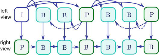
A video containing two or more views of the same scene, where each view is a single video sequence, is MV 3D video. Unlike the FC 3D video format, where each of the frames has full high definition (HD) [5, 29], more video sequences within a video lead to a significant increase in the amount of data, that is. the required bandwidth for transmission. In order to reduce the amount of data of the MV 3D video, during its coding, in addition to temporal and spatial redundancy within one view of the scene, the redundancy that largely exists between views is also used. The concept with interview prediction was included in the H.264/AVC standard as an amendment multiview video coding (MVC) [5]. Within this coding, intra-coded (I) frames, predictive (P) frames, and bi-directive (B) frames are used for reference frames, as shown in Figure 1.

Figure 1.

Illustration of interview prediction between views in MV 3D video.

3D video formats that, in addition to video sequences, contain additional depth data are MVPD video formats. Additional depth data is placed on the map based on the distance value of a point on the scene in the image plane to the camera. Using the depth matrix makes it much easier to create artificial views of the scene, but creating precise depth values is very complex. The advantage of depth video is direct compatibility with existing 2D systems.

Video with multiple video sequences has a significantly larger amount of data, so to improve this feature LVPD format was created, where image data from different views and depth data from different views placed in layers with the aim of reducing redundancy. Image information is reduced by projecting images from different views onto each other and eliminating repetitive content [30, 31, 32]. This procedure is repeated for depth data as well. In addition to the main layers, additional data about hidden elements of the scene are created in the image domain and in the depth domain.

Support for 3D video formats with depth is provided by the standard MPEG-C Part 3. This format requires the synthesis of additional views of the scene on the receiver side.

3. Video traffic using video traces

3.1 Video traffic characterization

There are generally three approaches to analyze video traffic in communication networks: using video bit stream, using video traces, and using a video transport model.

After encoding, a video bit stream is obtained with the selected encoder parameters. This data can be used for subjective and objective evaluations of video quality, as well as for video traffic analysis. During these analyses, the documents used are of the order $\mathrm{GB}$, which greatly complicates the examination. Also, most of the video material is proprietary, which limits research.

Based on the coded video material, it is possible to create a video trace, where the specific bits in the video bit stream are not saved but the information at the frame level. This approach does not violate the rights of the video owner.

The characterization of video sequences includes the determination of statistical characteristics of video signal traffic at the frame level and at the level of a group of images, as well as quality characteristics [13, 33]. These parameters are determined based on traffic metrics, quality metrics, as well as by rate-distortion (RD) and variability distortion (VD) curves [33].

3.2 Creating video traces

The creation of video traces begins by feeding the video signal to the reference encoder, which parameters can be changed. As a result of encoding, an encoded bit stream and a video trace document are obtained. Video trace documents are most often used to test the effectiveness of the coding method and to characterize the traffic of video material [33].

To generate YUV uncompressed video content from the stored video content, conversion software can be used, such as FFmpeg. A video trace can also be generated on the basis of pre-encoded video content present on the Internet, for example, using the software tool MPlayer.

Video traces for long video sequences, suitable for traffic evaluation, are available online thanks to researchers. Good examples are the database of the Technical University of Berlin published by Fitzek and Reisslein (http://www-tkn.ee.tu-berlin.de/research/trace/trace.html) and the video database Arizona State University traces credited by Reisslein, Karam, Seeling, Fitzek, and Madsen (http://trace.eas.asu.edu).

3.3 Structure of video traces

Video traces contain data about encoded video content. There are two types of video traces: video traces for frame sizes and video traces for frame quality.

A video trace document is typically a text document with ASCII (American Standard Code for Information Interchange) or unicode characters. At the beginning of the document, there is a header that gives general data about the video, and below is the video trace data in tabular form [33].

The video trace document header usually contains video title, frame format— spatial resolution, and frame rate, encoding method and encoder used, group of picture (GoP) organization, quantization parameter values, and basic statistical data.

Each row of the tabular part of the trace refers to one frame in the video. The first column contains the frame numbers $n=0,\dots ,N-1$, the second the display time of the frame $t_n$ in cumulative form, $t_n=\mathit{nT}$, and the type of frame (I, P, or B) in the third column. The size of the frames is described by the parameter $X_n^q$, which carries information about the number of bytes in the $n$th frame that is compressed with the quantization parameter $q$. In the video trace, for each of the frames, the quality is expressed within the parameters $Q_n^{q,Y}$, for the luminance component, and $Q_n^{q,U}$$Q_n^{q,V}$, for chrominance components.

In addition to the above data, the video trace can also contain additional data such as offset distortion and scores for the video quality metric, as well as the ordinal number of views to which the frame belongs in 3D video.

3.4 Parameters of analyzed 3D video sequences

An overview of the parameters of the examined 3D video formats is given in Table 1. MV, FS, and FC SBS 3D video formats were investigated using long, publicly available, video traces encoded using JMVC version 8.3.1, that is. H.264 reference software JSVM version 9.19.10 in single-layer encoding mode. The tested 3D video had two views ($V=2$), a left view (LV) and a right view (RV), where each view has 51,200 frames in full HD resolution ($1920\times 1080$) and frame rate $f=24\text{frames}/\mathrm{s}$. Tim Burton’s film Alice in Wonderland, which is a combination of real and computer-generated film, was used to evaluate the performance of 3D video. The analysis included different encoder settings for quantization parameters: $q_p=\left(I,P,B\right)$: $\left(\mathrm{24,24,24}\right)$, $\left(\mathrm{28,28,28}\right)$_, and $\left(\mathrm{34,34,34}\right)$. The length of a group of picture (GoP) for MV and SBS format is 16 frames, while for FS format it is 32 frames, which allows equal display time between adjacent I frames for each format. The picture group scheme is B1, which means that one B frame is located between consecutive I and P frames. Additionally, for MV 3D video GoP G16B7 was analyzed. The test also included determining the characteristics of video sequences for individual types of frames.

Parameter	LV	RV	MV	SBS	FC
Frame rate $f\left[\text{frames}/\mathrm{s}\right]$	24	24	48	24	48
Frame format	HD $1920\times 1080$
Number of frames	51,184	51,184	102,368	51,184	102,368
Video standard	H.264/AVC MVC			H.264/AVC
Encoder	JMVC 8.3.1			JSVM 9.19.10
Quantization parameters $q_p\left(I,P,B\right)$	$\left(\mathrm{24,24,24}\right)$, $\left(\mathrm{28,28,28}\right)$, $\left(\mathrm{34,34,34}\right)$
Group of Pictures, GoP	G16B1, G16B7				G32B1

Table 1.

Parameters of analyzed 3D video sequences.

In addition to examining the 3D video formats, the research included the determination of characteristics for 3D video with different streaming methods. Frames can be transmitted in their original form one by one or view-by-view for MV video when the LV and RV are viewed individually as separate video sequences. The second streaming method implies that certain views are combined, sequentially (S) or with aggregation (combining, C). In the case of sequential merging, frames from individual views are used to create a single sequence with the following frame order: frame 1 from view 1, frame 1 from view 2, …, frame 1 from view $V$, frame 2 from view 1, frame 2 from view 2, … In the case of merging with aggregation, MV frames are formed, where one MV frame represents the sum of all frames with the same serial number from different views. This principle was applied at the level of aggregation with two frames (marked as MV-C 2 and FS-C 2) and at the level of aggregation with the length of a group of images (MV-C 16 and FS-C 16).

4. Complex system theory

4.1 Fundamentals of complex systems

A complex system represents a network of individual components without central control, where simple individual components and their actions lead to complex behavior of the system as a whole, to sophisticated information processing, and possibilities for development and potentially adaptation.

Examples of complex systems include many natural and made systems such as insect colonies, neural networks, immune systems, cities, economic markets, and communication networks [34, 35].

One of the basic geometric properties of these systems is great complexity and fine structure regardless of the scale of observation [14]. By using fractal geometry, it is possible to measure the complexity of the system [36].

4.2 Fractals and fractal dimensions

Fractals represent complex geometric shapes, which have a fine structure on an arbitrarily small scale. Fractals usually have a certain degree of self-similarity, which can be exact or statistical [14, 37].

In order to measure the degree of complexity, it is necessary to find a relationship between how quickly the length, area, or volume change with decreasing scale. This would further allow determining the required size depending on the scale. The law that gives this relationship is a power law in the form

$$y\sim x^D.$$E1

This law is the basis of the fractal self-similarity dimension, which is defined as:

$$D=\frac{logm}{logr},$$E2

where $m$ is the number of copies, and $r$ is the scaling factor.

The principle of measuring complexity using the fractal self-similar dimension is simple to calculate, but for the case, where fractals do not scale, a generalized definition of the fractal dimension—box dimensions is needed.

Calculating the box dimension involves placing a complex structure on the grid whose boxes are $\epsilon$ in size and counting the boxes that contain part of the structure $N\left(\epsilon \right)$. By reducing the size of the $\epsilon$ box, a correspondingly larger value for $N\left(\epsilon \right)$ is determined. By plotting the obtained values on a log/log diagram and determining the slope of the line passing through the measured values, the box dimension is obtained.

In addition to the listed dimensions, which are used the most, there are other dimensions such as the pointwise dimension, a correlation dimension, and the Hausdorff dimension [14, 38].

4.3 Multifractals and multifractal spectra

In some situations, it is necessary to associate a certain measure with part of the set. Such as fractal sets, measure sets are considered to be highly irregular and variable in their value at different scales. If the variability of these sets is exactly or statistically self-similar, we are talking about multifractals [39].

To characterize the complexity of multifractals is necessary to include weighting coefficients that will depend on the value of the measure $\mu$.

The size $\alpha$ defined as

$$\alpha =\frac{log\mu \left(\mathrm{box}\right)}{log\left(\epsilon \right)}$$E3

represents the coarse Hölder exponent. The parameter $\alpha$ gives the ratio of the logarithm of the measure within the box to the logarithm of the size of the box. Typically, the coarse Hölder’s exponent $\alpha$ has values in the range $\left[{\alpha }_{\mathit{min}},{\alpha }_{\mathit{max}}\right]$, where $0<{\alpha }_{\mathit{min}}<{\alpha }_{\mathit{max}}<\infty$.

Once the parameter $\alpha$ is determined, it is necessary to determine its frequency distribution. For different values of the parameter $\alpha$, the number of boxes $N_{\epsilon }\left(\alpha \right)$ that have a rough Hölder exponent equal to $\alpha$ is determined. As in the determination of features of the original set, and with the parameter $\alpha$ the probability distribution with decreasing box size $\epsilon \to 0$ has no limiting value. Therefore, a weighted logarithmic function is needed.

$$f_{\epsilon }\left(\alpha \right)=-\frac{log{N}_{\epsilon }\left(\alpha \right)}{log\left(\epsilon \right)}.$$E4

This function for $\epsilon \to 0$ tends to the function $f\left(\alpha \right)$.

The function $f\left(\alpha \right)$ describes how with the decrease in the size of the boxes $\epsilon$, the number of boxes with a coarse Hölder exponent equal to $\alpha$, $N_{\epsilon }\left(\alpha \right)$ The connection of these parameters is given by the relation $N_{\epsilon }\left(\alpha \right)\sim {\epsilon }^{-f\left(\alpha \right)}$. The function $f\left(\alpha \right)$ describes the distribution of the parameter $\alpha$. The graph $f\left(\alpha \right)$ is denoted as multifractal spectrum or $f\left(\alpha \right)$ curve.

Sometimes the parameter $\alpha$ is denoted as the strength of the singularity and then $f\left(\alpha \right)$ represents the singularity or the Hausdorff singularity, and the $f\left(\alpha \right)$ curve is denoted as the spectrum of the singularity. The singularity $\alpha$ tracks local changes in the signal and $f\left(\alpha \right)$ gives the global characteristics of the data [39, 40, 41].

For an empirical self-similar measure, only one $n$-th state of the measure is known. In this case, in order to determine the multifractal spectrum, the previous states of the measurement are reconstructed by coarse-graining of the measurement. For discrete data, the smallest measure is obtained for the $n$-th measure state when the size of the boxes is $\epsilon =1$. The sum of all measures within a state equals one or is normalized to one.

To estimate multifractal characteristics and multifractal spectra of 3D video formats, the histogram method is used. This method is characterized by slower convergence of $f_{\epsilon }\left(\alpha \right)$ to $f\left(\alpha \right)$ and slower execution but can enable the display of additive processes in the signal and enables inverse multifractal analysis—determining the exact pieces of data that have a selected pair of values ($\alpha$, $f\left(\alpha \right)$). The histogram method works all the time with pure original data and contains fewer approximations.

5. Self-similarity analysis of 3D video formats

In this research, the fractal self-similarity of 3D video formats was examined using visual and rigorous statistical methods [19].

5.1 Self-similarity parameters

A process with values $X\left(t\right)$, $t\in \mathrm{ℝ}$ is self-similar with parameter $H$ if for each positive factor, $c$ the distributions of finite dimensions are $X\left(\mathit{ct}\right)$, $t\in \mathrm{ℝ}$, equal to the distribution $c^{H}X\left(t\right)$, $t\in \mathrm{ℝ}$ [14, 17]. Thus, typical self-similar series or self-similar processes look qualitatively the same regardless of the time scale on which they are observed. This does not mean that the same image is repeated in an identical way, but it is a general impression that the process remains the same.

One of the advantages of the self-similar model is that the degree of self-similarity is expressed by only one number, the $H$ parameter. This parameter is also referred to as the Hurst exponent or Hurst index. The values of the Hurst parameter can be divided into three categories [14, 42], where range $0<H<1/2$ stands for short-range dependent (SRD) processes, $H=1/2$ for random walk, and range $1/2<H<1$ for long-range dependent (LRD) processes.

It is shown that the traffic in communication networks exhibits self-similar properties, by measuring self-similarity using the Hurst parameter. This parameter indicates the level of traffic explosiveness, where higher values of the parameter indicate greater traffic explosiveness [43].

5.2 Methods for testing self-similarity

Self-similarity testing methods include the aggregated variance method, the R/S statistic method, and the method based on the correlation of multifractal analysis and the Hurst parameter, that is. multiscale method and others [17, 43]. In this chapter, the results will be given using the R/S statistic method, which was previously successfully tested on a process with fractal Gaussian noise, with a predefined value of Hurst parameter.

The R/S statistic method involves the following steps. Data on frame sizes $X_n$, $n=1,\dots ,N$ are divided into $K$ nonoverlapping blocks. Then, the rescaled adjusted ranges $R\left(t_i,d\right)/S\left(t_i,d\right)$ are determined for multiple values of the parameter $d$, where $t_i=N/K\left(i-1\right)+1$ are the starting points of the blocks that fill condition $\left(t_i-1\right)+d\le N$,

$$R\left(t_i,d\right)=max\left\{0,W\left(t_i,1\right),\dots ,W(t_i,d)\right\}-min\left\{0,W\left(t_i,1\right),\dots ,W(t_i,d)\right\}$$E5

wherein,

$$W\left(t_i,k\right)=\sum _{j=1}^k{X}_{t_i+j-1}-k\left(\frac{1}{d}\sum _{j=1}^d{X}_{t_i+j-1}\right),k=1,\dots ,d$$E6

and $S^2\left(t_i,d\right)$ the variance of the data $X_{t_i},\dots ,X_{t_i+d-1}$. R/S values were determined for each value of the $d$ parameter. This number decreases with the increase in the value of the $d$ parameter, which is a consequence of the restrictions that exist for the $t_i$ values. By drawing a graph of the value $log\left(R\left(t_i,d\right)/S\left(t_i,d\right)\right)$ as a function $logd$, the so-called R/S diagram is obtained. The slope of the regression line of the R/S value provides an estimate of the Hurst parameter.

5.3 Results of 3D video self-similarity analysis

Frame size traces of MV 3D video are shown in Figure 2(a), as a relation between the size of the frames and their sequence number. The video trace is also shown for two smaller ranges of frame numbers in Figure 2(b) and (c). The selected ranges are marked in Figure 2. Qualitatively, the self-similarity of MV 3D video is observed in Figure 2.

Figure 2.

Frame size in relation to frame number for MV 3D video: (a) full frame size video trace, (b) enlarged section of part of the trace labeled as (a), and (c) further enlarged section of part of the trace labeled as (b).

This self-similarity test is only graphical, so more rigorous statistical methods are needed to show the self-similar nature of 3D video formats, such as R/S statistic method.

Graphic representation of the R/S statistic method is shown in Figure 3. This is an example of a plot used in the estimation of the Hurst parameter. Reference lines have been added to the graphs for comparison, specifically reference lines with slopes $k_1=1/2$ and $k_2=1$. The slope of the regression line $\beta$ was estimated using the method of least squares fit and the R/S statistical method $H=\beta$. Examples of $H$ parameter estimation given in Figure 3 refer to MV 3D video representation format with quantization parameters $q_p\left(I,P,B\right)=\left(\mathrm{28,28,28}\right)$.

Figure 3.

Evaluation of Hurst parameter for MV 3D video using R/S statistic method.

Complete Hurst index evaluation results for left view (LV), right view (RV), combined view (CV), multiview (MV) 3D video formats, side-by-side (SBS), and frame sequential (FS) format are given in Table 2. The values of the quantization parameters for all video formats are $q_p\left(I,P,B\right)=\left(\mathrm{28,28,28}\right)$. Based on the results given in Table 2, it is concluded that Hurst index for 3D video formats has large values, indicating a high level of long-range dependence process for 3D video content.

3D Video type	Video format	$H_{R/S}$
One video sequence	SBS	0.9601
One video sequence	FS	0.9881
Multiview video	LV	0.9627
Multiview video	RV	0.9774
Multiview video	CV	0.9737

Table 2.

Hurst index values for 3D video representation formats using the R/S statistic method.

The previous results apply to video content when frames are broadcast one by one. Table 3 gives the results for the analysis of self-similar nature for streaming 3D video where aggregation of frames in pairs (denoted by C-2) or aggregation at the level of group of pictures (denoted by C-16). The results show a self-similar LRD behavior of 3D video content with aggregation, but with generally smaller values of the Hurst parameter.

3D Video type	$H_{R/S}$	3D Video type	$H_{R/S}$	3D Video type	$H_{R/S}$
SBS-C 2	0.9504	FS-C 2	0.9860	CV-C 2	0.9811
SBS-C 16	0.8676	FS-C 16	0.8567	CV-C 16	0.8681

Table 3.

Comparison of Hurst index values for 3D video representation formats with frame pair aggregation (C 2) and GoP aggregation (C 16).

6. Multifractal analysis of 3D video formats

Video content is characterized by high variability and the appearance of explosiveness, especially in the case when the values of the encoder’s quantization parameters are constant. Characterization of traffic variability is possible with statistical methods, such as coefficient of variation, RD, and VD curves. The dynamics and tendencies of fractal structure changes can be described using self-similarity parameters, as was done for 3D video in Chapter 5.3.

The mentioned characterizations of 3D video formats are very significant, but for the complete characterization of 3D video, multifractal analysis is also necessary due to the complexity of the video process. Also, this method enables a more precise insight into the behavior of the signal and its variability when broadcasting frame-by-frame or view-by-view, and gives particularly important results for broadcasting with frame aggregation. Such a more precise characterization of the 3D video format can allow for better modeling of this type of traffic, as well as for improving the efficiency of video transmission methods.

Multifractal characterization of 3D video signals is given in Refs. [23, 24, 25].

6.1 Estimation of multifractal properties by histogram method

In this research, the histogram method was used for multifractal characterization of 3D video formats.

The histogram method for determining the multifractal spectrum starts with overlaying a self-similar measure with boxes of size $\epsilon$. In the case of this method, $f_{\epsilon }\left(\alpha \right)$ slowly tends to $f\left(\alpha \right)$, so for a better estimation of the spectrum, sliding boxes were used to cover the measure instead of nonoverlapping ones.

In this analysis, $n_{\epsilon }=8$ of different box sizes were used, with the following values $\epsilon =\left[\mathrm{1,3,5,9,13,21,29,37}\right]$, that is, indices for ${\epsilon }_k$ are $k=1,2,\dots ,n_{\epsilon }$. For each value of ${\epsilon }_k$, the overall measure, ${\mu }_{i,k}$, where $i=1,2,\dots ,n$ is determined. The total length of the data and the value for ${\epsilon }_k$ determine the parameter $n$, where a larger number of existing measures is obtained for smaller boxes. For more efficient computation, all measurements are placed in a matrix $M$, where the size of the matrix is given by $\left[n_{\epsilon }\times n\right]$, for the largest possible $n$ (the smallest value for ${\epsilon }_k$). The coarse Hölder’s exponent ${\alpha }_i$, $i=1,2,\dots ,n$ is now determined as the slope for the graph $log\left({\mu }_i,k\right)$ in relative to $log\left({\epsilon }_k/L\right)$, where $L$ is the length of one-dimensional data.

The range of $\alpha$ values, $\left[{\alpha }_{\mathit{min}},{\alpha }_{\mathit{max}}\right]$ is discretized into $D=100$ parts of equal length $\mathrm{\Delta }\alpha$, and the ${\alpha }_d$ values are formed based on interval center values. In the domain of the parameter $\alpha$ of the value ${\alpha }_i$, for different values $j,j=\mathrm{1,3,5},\dots ,199$, the number $N_j\left({\alpha }_d\right)$ is determined as the number of boxes of size $j$_, which have the value ${\alpha }_i$ in the region $\mathrm{\Delta }\alpha$ around ${\alpha }_d$. This procedure is repeated for all values of ${\alpha }_d,d=1,2,\dots ,100$. Finally, the $f\left({\alpha }_d\right)$ values are determined as the slopes of the graph $-log\left(j/n\right)$ versus $log\left(N_j\left({\alpha }_d\right)\right)$. A plot of $f\left({\alpha }_d\right)$ versus ${\alpha }_d$ represents an estimate of the $f\left(\alpha \right)$ curve.

To understand the discussion of multifracral properties, it is important to know that ${\alpha }_{\mathit{min}}$ corresponds to the largest values of the measure, while ${\alpha }_{\mathit{max}}$ is associated with the smallest and smoothest part of the signal under investigation.

6.2 Results of multifractal analysis of 3D video format

3D video representation formats were examined in a multifractal sense using the histogram method. Multifractal video spectra are determined considering different multiview video views, different 3D video formats, different video streaming approaches, frame types, and GoP organization.

Multifractal spectra determined using the histogram method for different views of multiview 3D video and for different 3D representation formats are given in Figure 4(a) and (b), respectively. Multiview 3D video views have different data complexity (sequences of frame sizes), where RV has the lowest complexity, while CV and LV have similar, higher complexity, as seen by the range of dimensions in the spectrum. Also, the maximum of the multifractal spectrum for RV is the largest (the case with the highest frequency), while the singularity $\alpha \left(f_{\mathit{max}}\right)$ is the smallest compared to LV and CV. Multifractal spectra for CV multiview 3D video, FS, and SBS 3D representation formats show that the widest spectrum (most complex structure) occurs for CV, followed by SBS, while the least complexity is found in FS format.

Figure 4.

Multifractal spectra obtained using the histogram method: (a) different representational formats of 3D video and (b) different views for MV 3D video — Left, right, and combined.

The multifractal spectrum for RV has two dominant peaks at the top of the spectrum, which is due to the two processes that exist within the data— the P and B frames in the signal formed using the frames from the LV as a reference. A similar, but less pronounced process is present in the case of the spectrum for CV of MV 3D video.

Multifractal spectra obtained by applying the histogram method for selected types of frames: Only I frames, only P frames, and only B frames for different 3D video representation formats are given in Figure 5. The smallest changes in the multifractal spectrum are observed for I frames as a consequence of the similar coding principle of this type of frame, regardless of the 3D video format. The maximum of the multifractal spectrum is the smallest in the case of I frames, followed by the maximum for B-type frames and P-type frames. The smallest decrease of the multifractal spectrum around its maximum was observed for I frames, which is a consequence of the structure with a larger number of dimensions whose participation in the structure is significant. Multifractal spectra for P and B frames have a faster decay and fewer dimensions with a large participation in the signal. For isolated frame types, sequences with only P frames have a multifractal spectrum with the smallest value of the ${\alpha }_{\mathit{min}}$ parameter, which means the highest explosiveness. Similar conclusions can be drawn based on the multifractal spectra obtained using the moment method. The relationships between multifractal spectra for CV, SBS, and FS formats for I-only, P-only, and B frames are the same as for video sequences with all frame types.

Figure 5.

Multifractal spectra obtained by the histogram method for selected types of frames: (a) only I frames for 3D video representation formats, (b) only I frames for different views of MV 3D video, (c) only P frames for 3D video representation formats, (d) only P frames for different views of MV 3D video, (e) only B frames for 3D video representation formats, and (f) only B frames for different views of MV 3D video.

Comparison of multifractal spectra of MV 3D video with different groups of picture (GoP) organization is given in Figure 6. GoP with higher number of B frames shows slightly less additive processes in signal, but width of multifractal spectra stays approximately the same.

Figure 6.

Multifractal spectra by the histogram method: (a) MV 3D with GoP G16B1 and GoP G16B7, (b) RV 3D with GoP G16B1 and GoP G16B7.

As given in Ref. [13] based on CoV, the FS 3D format has better properties in terms of variability than the MV 3D format, but with frame aggregation (for a pair of consecutive frames or for 16 consecutive frames—one GoP) video sequences show better characteristics in terms of variability for both formats, especially for MV 3D video which becomes more similar in characteristics to the FS format. These results were further analyzed in terms of the explosiveness of the video signal, which is very important for data traffic. Video sequences with frame aggregation were also analyzed using the multifractal spectrum obtained using the histogram method. These results are shown in Figure 7. The main change on the spectrum, for video content with aggregation, is the position of the spectrum maximum $\alpha \left(f_{\mathit{max}}\right)$, which represents the complexity of the structure in the case with the highest frequency. Both 3D formats, FS and CV, have a less complex structure, a smaller value of $\alpha$ in the case with the highest frequency, for sequences with aggregation. A small improvement was observed for aggregation at the level of two frames, while a larger improvement was observed for aggregation at the new group of images. The parameter $f_{\mathit{max}}$ for FS and CV spectra is very similar.

Figure 7.

Multifractal spectra by the histogram method for MV and FS video with aggregation.

7. Conclusions

In this book chapter, 3D video representation formats are characterized: multiview (MV) video representation format that uses multiview video coding, as well as frame sequential (FS) and frame compatible (FC) and side-by-side (SBS) formats that use encoding using a conventional single-view video encoder. The analysis of 3D video formats is realized using 3D video traces for these three main 3D video representation formats. Publicly available traces of long video sequences [12, 13] were used. Video traces contained information about each individual video frame: display time, frame size, frame type, and frame quality parameters. Within one 3D video sequence for one setting of quantization parameters, there were two views with 51,200 frames each in full HD $1920\times 1080$ (resolution)

In this book chapter, several aspects regarding fractal and multifractal characterization of 3D video are presented.

An essential overview of 3D video representation and compression formats according to fractal and multifractal properties is given [19, 25].

It has been shown that video sequences of 3D video format have fractal self-similar properties with long-range dependence (LRD) [19]. The characterization of the fractal properties of 3D video was realized using a visual method and detailed calculation using R/S statistic method using codes implemented in MATLAB and Python, which showed high values of the Hurst parameter of about $0.95$ indicating a high-level explosiveness and LRD characteristics [19].

It is shown that the three main examined 3D video formats have a multifractal structure [23, 24, 25], as well as individual views in multiview 3D video format using the multifractal spectra. The implementation of the algorithm and the application of the histogram method using codes written in the MATLAB and Python [25] showed that MV video has the most pronounced multifractal structure for the most pronounced singularity (the largest part of the structure), while the least pronounced multifractal nature is present in FS video.

An overview of the fractal and multifractal properties of the 3D video format depending on the choice of frame type was given, which showed a great similarity of the multifractal properties of the intra-coded (I) frames of the 3D video format, which is a consequence of the similar coding principle of this type of frame, and which showed differences in the variability of frame types, especially pronounced for prediction (P) coded and bidirectional (B) coded frames for different 3D video formats, which is a consequence of different coding approaches, as well as the highest explosiveness of P-type frames [22, 23, 25].

Fractal and multifractal properties of 3D video representation formats in the case of frame aggregation and in different conditions of 3D video broadcasting were exposed with the aim of determining more efficient transmission, which showed a decrease in the expression of variability if only certain generalized dimensions or fractal self-similarity are observed, but an increase in explosiveness on a smaller to the part of the signal that is observed thanks to the multifractal spectrum [19, 25].

Values of fractal and multifractal parameters of 3D video representation formats could be used for modeling 3D video traffic in communication systems [17, 19, 20, 25, 37, 39].

The results presented in this chapter can be used to improve methods of reducing variability (smoothing) and to design more efficient multiplexing methods, in applications such as smoothing with pre-sending part of the signal [44], more precisely in terms of explosive traffic estimation and its management process and controls.

Statistical multiplexing methods that use frame type information to improve features can potentially improve performance given the multifractal features of the different frame types presented in this book chapter [22, 23, 25]. Also, the results can be used in examining the impact of the introduction of 3D video formats into the multiplexer with 2D video formats on the channel characteristics.

References

1.Merkle P, Müller K, Wiegand T. 3D video: Acquisition, coding, and display. IEEE Transactions on Consumer Electronics. 2010;56(2):946-950
2.Rocha L, Gonçalves L. An overview of three-dimensional videos: 3D content creation, 3D representation and visualization. In: Bhatti A, editor. Current Advancements in Stereo Vision. Rijeka: IntechOpen; 2012
3.Eisert P, Schreer O, Feldmann I, Hellge C, Hilsmann A. Volumetric video – acquisition, interaction, streaming and rendering. In: Valenzise G, Alain M, Zerman E, Ozcinar C, editors. Immersive Video Technologies. Cambridge, Massachusetts: Academic Press; 2022. p. 289-326
4.Kerdranvat M, Chen Y, Jullian R, Galpin F, François E. The video codec landscape in 2020. In: The future of video and immersive media. ICT Discoveries. International Telecommunication Union. 2020;3(1):73-84
5.Tech G, Chen Y, Müller K, Ohm JR, Vetro A, Wang YK. Overview of the multiview and 3D extensions of high efficiency video coding. IEEE Transactions on Circuits and Systems for Video Technology. 2016;26(1):35-49
6.Karsten Müller PE, Schwarz H, Wiegand T. Video Data Processing. Heidelberg, Germany: Springer-Verlag - part of Springer Nature; 2019
7.Punchihewa A, Bailey D. A review of emerging video codecs: Challenges and opportunities. In: 2020 35th International Conference on Image and Vision Computing New Zealand (IVCNZ). Wellington, New Zealand: IEEE. 2020. pp. 1-6
8.Mohib H, Swash MR, Sadka AH. Multi-view video delivery over wireless networks using HTTP. In: Proceedings of International Conference on Communications, Signal Processing, and their Applications. Sharjah, United Arab Emirates: IEEE; 2013. pp. 1-5
9.Malekmohamadi H. Automatic subjective quality estimation of 3D stereoscopic videos: NR-RR approach. In: 3DTV Conference: Capture, Transmission and Display of 3D Video. Copenhagen, Denmark: IEEE; 2017. pp. 1-4
10.Tanwir S, Nayak D, Perros H. Modeling 3D video traffic using a Markov modulated gamma process. In: 2016 International Conference on Computing, Networking and Communications (ICNC). Kauai, HI, USA: IEEE; 2016. pp. 1-6
11.Hao J, Liu S, Guo B, Ding Y, Yu Z. Context-adaptive online reinforcement learning for multi-view video summarization on Mobile devices. In: 2022 IEEE 28th International Conference on Parallel and Distributed Systems (ICPADS). Nanjing, China: IEEE; 2023. pp. 411-418
12.Video Trace Library. Available from: http://trace.eas.asu.edu.
13.Pulipaka A, Seeling P, Reisslein M, Karam L. Traffic and statistical multiplexing characterization of 3D video representation formats. IEEE Transactions on Broadcasting. 2013;59(2):382-389
14.Peitgen H, Jürgens H, Saupe D. Chaos and Fractals. New York: Springer; 1992
15.Ingole AV, Kamble SD, Thakur NV, Samdurkar AS. A review on fractal compression and motion estimation techniques. In: 2018 International Conference on Research in Intelligent and Computing in Engineering (RICE). San Salvador, El Salvador: IEEE; 2018. pp. 1-6
16.Tiwari M, Chaurasia V, Siddiqui EA, Patel V, Kumar A, Patankar M. Enhanced image compression using fractals and principle component analysis. In: 2023 1st International Conference on Innovations in High Speed Communication and Signal Processing (IHCSP). Bhopal, India: IEEE; 2023. pp. 502-507
17.Sheluhin O, Smolskiy S, Osin A. Self-Similar Processes in Telecommunications. New York: John Wiley & Sons, Inc.; 2007
18.Filaretov GF, Chervova AA. Fractal characteristics of the network traffic. In: 2022 VI International Conference on Information Technologies in Engineering Education (Inforino). Moscow, Russian Federation: IEEE; 2022. pp. 1-4
19.Zekovic A, Reljin I. Self-similar nature of 3D video formats. In: Jonsson M, Vinel AV, Bellalta B, Belyaev E, editors. Proceedings of Multiple Access Communications - 7th International Workshop, MACOM 2014, Halmstad, Sweden, August 27–28, 2014. Lecture Notes in Computer Science series. Vol. 8715. New York City, USA: Springer; 2014. pp. 102-111
20.Dang TD, Molnár S, Maricza I. Capturing the complete multifractal characteristics of network traffic. In: Global Telecommunications Conference. Taipei, Taiwan: GLOBECOM IEEE; 2002. pp. 2355-2359
21.Millán G, Osorio-Comparán R, Lomas-Barrie V, Lefranc G. The associative multifractal process: A new model for computer network traffic flows. In: IEEE Chilean Conference on Electrical, Electronics Engineering, Information and Communication Technologies. Valparaíso, Chile: IEEE; 2021. pp. 1-6
22.Zekovic A, Reljin I. Multifractal and inverse multifractal analysis of multiview 3D video. In: Proceedings of 21st Telecommunication Forum (TELFOR 2013), 26–28 November 2013; Belgrade, Serbia: TELFOR; 2013. pp. 753-756
23.Zekovic A, Reljin I. Inverse multifractal analysis of different frame types of multiview 3D video. TELFOR Journal. 2014;6(2):121-125
24.Zekovic A, Reljin I. Comparative analysis of multifractal properties of H.264 and multiview video. In: Proceedings of 1st International Conference on Electrical, Electronic and Computing Engineering IcETRAN 2014, 2–5 June 2014; Vrnjačka Banja, Serbia: IcETRAN; 2014. pp. EKI1.7.1-4
25.Zekovic A, Reljin I. Multifractal analysis of 3D video representation formats. EURASIP Journal on Wireless Communications and Networking. 2014;2014(181):1-14
26.Smolic A. 3D video and free viewpoint video – From capture to display. Pattern Recognition. 2011;44(9):1958-1968
27.Zhang C, Su M, Liu Q, Yang M. 3D communication system integrating 3D reconstruction and rendering display. In: 2022 5th International Conference on Advanced Electronic Materials, Computers and Software Engineering (AEMCSE). Wuhan. China: IEEE; 2022. pp. 167-170
28.Patil VTM, Anami B, Billur D. Effective 3D video streaming using 2D video encoding system. In: 2022 2nd Asian Conference on Innovation in Technology (ASIANCON). Ravet. India: IEEE; 2022. pp. 1-5
29.Müller K, Merkle P, Tech G, Wiegand T. 3D video formats and coding methods. In: Proceedings of the 17th IEEE International Conference on Image Processing (ICIP): 26–29 September 2010; Hong Kong, China: IEEE; 2010. pp. 2389-2392
30.Cagnazzo M, Pesquet-Popescu B, Dufaux F. 3D video representation and formats. In: Dufaux F, Pesquet-Popescu B, Cagnazzo M, editors. Emerging Technologies for 3D Video: Creation, Coding, Transmission and Rendering. New Jersey, USA: Wiley Publishing; 2013
31.Yilmaz GN, Battisti F. Depth perception prediction of 3D video for ensuring advanced multimedia services. In: 2018 - 3DTV-Conference: Capture, Transmission and Display of 3D Video. Helsinki, Finland: IEEE; 2018. pp. 1-3
32.Merkle P, Müller K, Marpe D, Wiegand T. Depth intra coding for 3D video based on geometric primitives. IEEE Transactions on Circuits and Systems for Video Technology. 2016;26(3):570-582
33.Seeling P, Fitzek FHP, Reisslein M. Video Traces for Network Performance Evaluation. Dordrecht: Springer; 2007
34.Mitchell M. Complexity: A Guided Tour. Oxford, New York: Oxford University Press; 2009
35.Easley D, Kleinberg J. Networks, Crowds, and Markets: Reasoning about a Highly Connected World. Cambridge, United Kingdom: Cambridge University Press; 2010
36.Lloyd S. Measures of complexity: A non-exhaustive list. IEEE Control Systems Magazine. 2001;21(4):7-8
37.Feder J. Fractals. New York: Springer Science – Business Media; 1988
38.Strogatz SH. Nonlinear Dynamics and Chaos: With Applications to Physics, Biology, Chemistry, and Engineering. Cambridge, Massachusetts: Westview Press; 2001
39.Evertsz A, Mandelbrot B. Multifractal Measures. In: Peitgen H, Jürgens H, Andrews P, editors. Chaos and Fractals. New York: Springer; 1992. pp. 849-881
40.Véhel JL, Tricot C. On Various Multifractal Spectra. Progress in Probability. 2004;57:23-42
41.Chhabra A, Meneveau C, Jensen V, Sreenivasan K. Direct determination of the f(α) singularity spectrum and its application to fully developed turbulence. Physical Review A. 1989;40(9):5284-5294
42.Mandelbrot BB, van Ness JW. Fractional Brownian motions, fractional noises and applications. SIAM Review. 1968;10:422-437
43.Leland W, Taqqu M, Willinger W, Wilson DV. On the self-similar nature of Ethernet traffic (extended version). IEEE/ACM Transactions on Networking. 1994;2(1):1-15
44.Devi UC, Kalle RK, Kalyanaraman S. Multi-tiered, Burstiness-aware bandwidth estimation and scheduling for VBR video flows. IEEE Transactions on Network and Service Management. 2013;10(1):29-42
Written By
Amela Zekovic
Submitted: 11 June 2023Reviewed: 30 June 2023Published: 14 September 2023
Open access peer-reviewed chapter