Topology Optimization Generating System

Abstract

In this project, we started with discussing the structural topology approaches in general throughout the concept of topology optimization. We discussed the different types of topologies and their mathematical functions, and then, we established the idea of creating the topology optimization generating system. We made a collaboration of multiple programs and algorithms to create a friendly user environment for mechanical engineers mostly to design their own work with the best optimized solution possible with the less available volume of material. Afterwards they can test the result with a physics simulator and apply any constrains and physical force anywhere they want.

1. Introduction

The structural optimization is considered to be a mechanical designing to be a mechanical designing concept. The main purpose behind it is to find the optimal type of structure considering the constrains applied on the structure target.

2. Optimization problem

The main concept behind the topology optimization problems is to find the variable x where it minimizes or maximizes the objective function f(x) considering the constrains applied to the initial structure. There are many methods to solve this problem by using an optimization model to solve our problem.

Every optimization model has the following [1]:

• Objective function $\mathit{f}\left(\mathit{x}\right)$:

  This function describes the structure goal that the user wants to optimize by finding the region of feasible solutions. Thus, the objective function job is to minimize or maximize the amount of manufacturing material in every micro-structure.

• Design variable $\left(\mathit{x}\right)$:

  The variable $\left(\mathit{x}\right)$ describes the parameters that the objective function depends on them, whereas the objective function searches for the best results to reach the optimal solution for the structure goal.

• Constrains:

  Having constrains in the optimization problems is conditional where it depends on each individual issue, but in real-life optimization problems, there must be few constrains to mark the feasible regions.

Figure 1 shows how the feasible regions can be different due to each optimization problem.

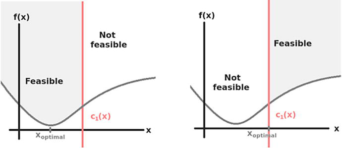
Figure 1.

Feasibility regions.

3. Structural optimization

The main idea behind the structural optimization is making an assemblage of materials to sustain loads in the best way possible, and thus, it is considered to be a mechanical designing process that aims to find the optimized structure considering the designing area [2].

4. The main types of structural optimization

• Size Optimization:

Size optimization is considered to be the simplest method where the optimization parameters are given by the structural parameters like height, width thickness and corners. In this method, the shape of the target is known, but the goal is to find a better shape. In this type, the structural elements are the design variables, and the objective function aims to find different shapes of the structure goal [2].

• Shape Optimization:

  This type is considered to be an extension of size optimization, whereas it allows us to set the range of the elements of material interdependence, and the goal of this method is to change rearrange the place of elements without changing the interdependency of the elements themselves. In this type, the parameters of the objective function are the coordinates of the structure corners considering few parameters to build the edges of the structure target like reducing the stress—decrease or increase the exertion applied on the structure…etc.

• Topology Optimization:

  This type is considered to be better than the other types because it does not apply constrains on the structure goal. In this type the design target can be partitioned into elements whereas the optimization parameters are a group of elements, these elements are the material parameters that shows the material variation where the structure goal has holes in it and were it does not. The objective function is to find the best way to variate the material.

5. Finite element method

This method is used to find a numeric solution for the differential equations. The main purpose behind solving them is to describe the behavior of any physical phenomenon, whereas we try to solve the elastic problem described by the displacement as a result of applying any force on the elastic initialized structure. The elasticity of the initialized structure can be static at certain elements. The main role of the finite element method is being linked with the topology optimization objective function and its constrains [3, 4].

In this method, we turn the initial structure into small pieces called the micro-structures, whereas any physical force applied on the initialized structure will have an effect on the micro-structures.

• Linear elastic problem:

  We implement the displacement field in the stress and strain problems as a two-way displacement field for each element in the designing area.

  The displacement vector is represented as

$$\mathrm{U}=\mathrm{U}\left(\mathrm{X},\mathrm{Y}\right)=\left[\begin{array}{c}u\left(x,y\right)\\ v\left(x,y\right)\end{array}\right]=\left[\begin{array}{c}u\\ v\end{array}\right]$$E1

Whereas each u and v represent the displacement on x, y coordinates at a specific element.

The strain can be calculated using the displacement vectors on the plane xy using the general elastic theory, whereas we implement the strain vector as.

$$\epsilon =\left[\begin{array}{c}{\epsilon }_x\\ {\epsilon }_y\\ {\gamma }_{\mathit{xy}}\end{array}\right]=\left[\begin{array}{c}\frac{\partial u}{\partial x}\\ \frac{\partial v}{\partial y}\\ \frac{\partial u}{\partial y}+\frac{\partial v}{\partial x}\end{array}\right]=\left[\begin{array}{cc}\frac{\partial }{\partial x}& 0\\ 0& \frac{\partial }{\partial y}\\ \frac{\partial }{\partial y}& \frac{\partial }{\partial x}\end{array}\right]\left[\begin{array}{c}u\\ v\end{array}\right]=\mathrm{Bu}$$E2

Whereas each ${\epsilon }_x$ and ${\epsilon }_y$ represent the normal strain on x, y coordinates, and ${\gamma }_{\mathit{xy}}$ represents the shear strain on the plane xy.

The stress vector:

$$\sigma =\left[\begin{array}{c}{\sigma }_x\\ {\sigma }_y\\ {\tau }_{\mathit{xy}}\end{array}\right]$$E3

Whereas each ${\sigma }_x$and ${\sigma }_y$ represent the normal stress on x, y coordinates, and ${\gamma }_{\mathit{xy}}$ represents the tangential stress on the plane xy.

The relationship between stress and strain represented as

$$\sigma =D\epsilon$$E4

In the general status:

$$\sigma =D\left(\epsilon -{\epsilon }_0\right)+{\sigma }_0$$E5

This equation reserves on the linear behavior until a certain limit called the elastic limit.

In the previous equation, D represents the basic matrix that has all the elasticity properties of the manufacturing material:

$$\mathrm{D}=\left[\begin{array}{ccc}{d}_{11}& d_{12}& 0\\ d_{21}& d_{22}& 0\\ 0& 0& d_{33}\end{array}\right]$$E6

Based on Maxwell–Betti theory, then D is symmetrical [5].

Using isotropic material, D can be calculated for stress as

$$d_{11}=d_{22}=\frac{E}{1-v^2}$$E7

$$d_{12}=d_{21}=v{d}_{11}$$E8

$$d_{33}=\frac{E}{2\left(1+v\right)}$$E9

The strain is calculated by

$$d_{11}=d_{22}=\frac{E\left(1-v\right)}{\left(1+v\right)\left(1-2v\right)}$$E10

$$d_{12}=d_{21}=d_{11}\frac{v}{1-v}$$E11

$$d_{33}=\frac{E}{2\left(1+v\right)}$$E12

Whereas E represents Young’s modulus, and $v$ represents the Poisson radius.

• Discrete Solution:

  This equation allows to represent the effect of the generated work done by the internal and external forces of the design and links the stress, strain and pressure:

$$\begin{array}{c}{\iint }_A\left(\delta {\epsilon }_x{\sigma }_x+\delta {\epsilon }_y{\sigma }_y+\delta {\gamma }_{\mathit{xy}}{\tau }_{\mathit{xy}}\right)\mathit{hdA}={\iint }_A\left(\mathit{\delta u}{b}_x+\mathit{\delta u}{b}_y\right)\mathit{hdA}\\ +{\iint }_s\left(\mathit{\delta u}{t}_x+\mathit{\delta v}{t}_y\right)\mathit{hds}+{\int }_i\left(\delta u_i{U}_i+\delta v_i{V}_i\right)\end{array}$$E13

This can be written in a matrix way:

$${\iint }_A\delta {ϵ}^T\mathit{\text{σhdA}}={\iint }_A\delta u^T\mathit{\text{bhdA}}+{\int }_s\delta u^T\mathit{\text{thds}}+\sum _i\delta u_i^T{q}_i$$E14

Whereas $\mathit{\delta u},\mathit{\delta ϵ},\sigma$ represent the theoretical vectors, the theoretical stress and the pressure fields.

$h$ represents the thickness of the initial structure.

$b,t,q$ represent the forces applied on the initial structure given by:

The forces applied on the structure elements:

$$b=\left[\begin{array}{c}{b}_x\\ b_y\end{array}\right]$$E15

The forces applied on the edges:

$$t=\left[\begin{array}{c}{t}_x\\ t_y\end{array}\right]$$E16

The forces applied on the points:

$$q=\left[\begin{array}{c}U\\ V_y\end{array}\right]$$E17

All these forces will be given as constrains for the optimization process.

Using finite element method, we can solve our problem using the discrete method where we calculate the solution at some points, then we interpolate the solution in the middle points, and thus, the elements will be generated from the points and the links between them and that is how we create a complete generation for the initial structure elements as shown in Figure 2:

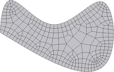
Figure 2.

Initial structure elements.

To apply the theoretical work of the elements depending on Eq. (2) that can be written as:

$${\iint }_{A^e}\delta u^T\mathit{\sigma hd}{A}^e={\iint }_{A^e}\delta u^T\mathit{bhd}{A}^e+{\int }_{s^e}\delta u^T\mathit{thd}{s}^e+\delta u^T{q}^e$$E18

Now, we can partition and except the theoretical work vectors since it is randomly generated from the work of elements equation:

$${\iint }_{A^e}{B}^T\mathit{\sigma hd}{A}^e={\iint }_{A^e}\mathit{bhd}{A}^e+{\int }_{s^e}\mathit{thd}{s}^e+q_e$$E19

Replacing the general Eq. (5) with the first part of the previous equation:

$${\iint }_{A^e}{B}^T\left(D\left(\epsilon -{\epsilon }_0\right)+{\sigma }_0\right)\mathit{hd}{A}^e={\iint }_{A^e}\mathit{bhd}{A}^e+{\int }_{s^e}\mathit{thd}{s}^e+q_e$$E20

Algebraically, we get

$$h{\iint }_{A^e}{B}^T\mathit{\epsilon d}{A}^e=h{\iint }_{A^e}{B}^{T}D{\epsilon }_{0}d{A}^e-h{\iint }_{A^e}{B}^T{\sigma }_{0}d{A}^e+h{\iint }_{A^e}\mathit{bd}{A}^e+h{\int }_{s^e}\mathit{td}{s}^e+q^e$$E21

Replacing Eq. (2) with the first part of the previous equation, we get

$$h{\iint }_{A^e}{B}^T\mathit{DBd}{A}^{e}u=h{\iint }_{A^e}{B}^{T}D{\epsilon }_{0}d{A}^e-h{\iint }_{A^e}{B}^T{\sigma }_{0}d{A}^e+h{\iint }_{A^e}\mathit{bd}{A}^e+h{\int }_{s^e}\mathit{td}{s}^e+q^e$$E22

This equation can be written as

$$K^e{u}^e=\left[f_{\in }^e-f_{\sigma }^e+f_b^e+f_s^e\right]+q^e=f^e+q^e$$E23

After assembling all the element wide matrices, we get this linear equation:

$$\mathrm{K}.\mathrm{u}=\mathrm{f}$$E24

6. Topology optimization mathematical function

We start by solving the linear equation:

$$\mathrm{K}.\mathrm{u}=\mathrm{f}$$E25

Whereas:

K is the stiffness matrix (determines the hardness of the material).

U is the displacement vector (determines where not to add material during design.)

f is the forces vectors.

The stiffness matrix K can be factorized as

$$\mathrm{K}=\mathrm{E}.\widehat{\mathrm{K}}$$E26

Whereas:

E is the Young’s parameter (determines the solidity of the structure).

$\widehat{\mathrm{K}}$ is the factorized stiffness matrix.

The main purpose behind dividing the stiffness matrix is to divide the structure goal into small parts to determine which element is more important than others. Now, we can factorize the elements using the equation:

$${\mathrm{k}}_{\mathrm{e}}=\mathrm{E}.{\widehat{k}}_{\mathrm{e}}$$E27

Whereas:

E is the Young’s parameter for each element e.

Now, we can link each element with any of the parameters of designing with each parameter from the constrains using this equation:

$${\mathrm{E}}_{\mathrm{e}}={\mathrm{x}}_{\mathrm{e}.}\mathrm{E}$$E28

Replacing E_e, we get:

$${\mathrm{k}}_{\mathrm{e}}={\mathrm{x}}_{\mathrm{e}.}\mathrm{E}.{\breve{k}}_{\mathrm{e}}$$E29

Thus, each variable x_e is considered to be a parameter for the topology optimization problems. When x_e = 1, we get material, when x_e = 0, we get an empty hole. Some methods use binary design variables, whereas others may use continuous values between 0 and 1.

Figure 3 shows how assigning the optimal values to the variables in topology optimization methods can give the best results:

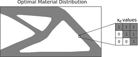
Figure 3.

Optimal Material Distribution.

7. Topology optimization approaches

• Density-Based Method (Gradient Methods) [6]:

  This method depends on creating a discrete designing space using solid elements or solid nodes, whereas it is available to change the volume of design or the stiffness of each micro-structure by changing the value of the variable x_e considering its range [x_min, x_max], and thus, we can create a physical simulation by changing the density or the solidarity(Young’s parameter).

• Solid Isotropic Material with Penalization (SIMP) [7]:

  This methodology is also gradient-based where it preserves on the solidity of the material. The structure goal should get fragmented into micro-structures so that the user can delete any unwanted parts from the initial structure, and in this method, the stiffness stays the same for each element, whereas we make several alignments to get to the structure goal. The algorithm of this method starts with setting the stiffness of all elements elected to be the same taking in consideration that all the selected elements have the same volume, and thus, the algorithm will frequently start setting the optimality of each element considering the constrains needed to be applied on the structure goal.

  This method was used in many researches like [5, 8, 9].

  SIMP algorithm steps:

1. Create initial structure fragments.

2. Set the micro-structure to be solid elements gradually.

3. Analyze the elements considering the physical constrains applied (forces, stress… etc).

4. Find the optimal value for each element considering how important is the element for the optimization process.

5. Reduce the number of elements frequently.

6. Use the “soft kill” penalization concept where each element has its own situation of material (has material—space—partly has material).

The pros of SIMP algorithm:

1. The initial structure does not have to be homogenous.

2. Considered to be mathematically functional.

3. Considered to be approximately flexible with any design.

4. Does not require hard mathematics understanding.

5. Can be used with any physics constrains.

The cons of SIMP algorithm:

1. Depends on the mesh of the material.

2. There might be elements with two types of materials.

3. Depends on penalization.

Figure 4 shows how SIMP algorithm works:

• Rational Approximation of Material Properties [7, 10]:

  This method has been established to fix the designs that takes the weather circumstances in consideration like: wind force, humidity, snow…etc., and the main concept behind it is to be an initial alternative formula of (SIMP) algorithm where the designer determines the designing void area as a hydro-static liquid unable to be pressured, the liquid transforms the pressure force without leaving any marks on the surface.

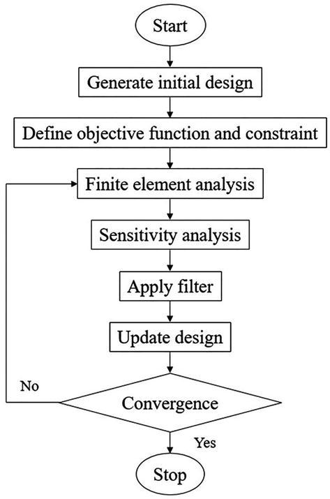
Figure 4.

SIMP Algorithm steps.

This method was used in many researches like [11, 12, 13].

The cons of RAMP:

• Depends on penalization.

• It shows hard mathematical problems when using low-stiffness structured elements.

Figure 5 clarifies the idea of RIMP:

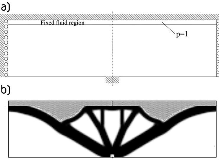
Figure 5.

RIMP Algorithm result.

Heuristic Methods (Discrete Methods) [6]:

This type depends on the knowledge of the user to get to the structure goal, and it is not necessary to have mathematical knowledge base. These methods considered to be simple, but on the other hand, reaching the local or global optimal results is not guaranteed because it does not change any of the variables or parameters of the structure goal considering the optimization algorithm applied on the initial structure.

These methods were used in many researches like [14, 15, 16].

Meta-Heuristic Methods [6]:

These methods considered to be randomized, and in many topology optimizing cases, these methods depend on population-based proof of concept where they are called evolutionary algorithms. Each element of structure is being evaluated by a randomizing solution, whereas the best elements are picked up by the algorithm to create the best evaluating solution. The main steps of these algorithms are selection, crossover, mutation and replacement applied on the chosen elements of structure.

These methods were used in many researches like (Figure 6) [17, 18, 19] .

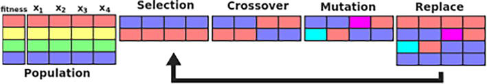
Figure 6.

Meta Heuristic methods work.

The pros of meta-heuristic methods:

• Capable of avoiding local optimal limitations.

• Capable of being approached from global optimal limitation.

• Does not need a lot of information about the initial structure.

The cons of meta-heuristic methods:

• Cannot handle a lot of variables about the initial structure.

• Require heavy types of computing resources.

8. Topology optimization generating system

The main purpose that stands behind this project is the need of reducing the amount of material used in manufacturing without weakening the structure goal, also making the designing process easier by adding the constrains strictions and physical behavior so that the structure goal became more mesh-linked and efficient. This project stands upon finding the best variation of the material of manufacturing in strict circumstances so that the structure goal has the same efficiency of the initial structure but less manufacturing material.

9. The functional requirements

• Choosing the initial structure:

  Using FreeCAD software, we managed to create a designer-friendly environment that gives the users all the freedom during their journey of designing the initial structure, whereas they can design their 3D model in any shape, volume and all the details they want or import a previous model they already have and apply their changes on it.

• Initial goal partition:

  In this part, we change the initial structure into a solid structure, and then, we applied the partitioning method that is called the finite elements method where the user can change then approve the method’s work.

• Apply the physical constrains:

  Using a plugin tool called “Calculix”, the designer can apply any type of physical constrains that he/she wants, like: material type, stiffness… etc.

• Apply the functional constrains:

  While using the plugin “Calculix”, the designer can apply the fixed points and the force vectors parameters like: the transformation and rotation of the vector and the intensity of force… etc.

• Managing the evacuation process:

  After applying all the constrain needed, the 3D model file would be an input file to the evacuation process with another parameters that the algorithm needs like the iteration number whether or not save all iterations… etc.

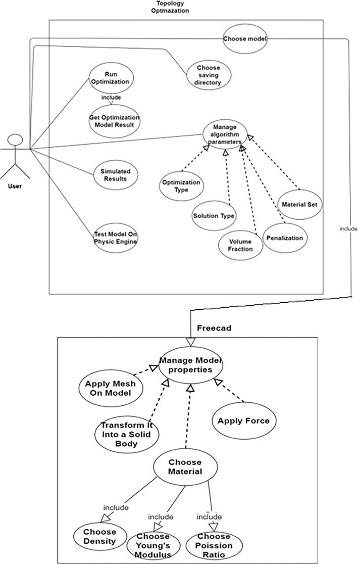
  For this level, we managed to implement the SIMP algorithm as a plugin to FreeCAD to create a user-friendly interface to manage all the parameters and constrains needed to be applied on the initial 3D model.

  The user interface includes:

1. Choose the path of saving all the iterated models that have been evacuated.

2. Set all the parameters of the SIMP algorithm.

3. Start the evacuation process.

4. Test the results on the physical simulator that will be explained later on.

5. Show the results of the most optimized 3D model.

6. Represent a GIF of all the iterations of the evacuation process.

7. Test the results using a physics simulator.

• The evacuation process works:

  Using the solid isotropic material with penalization (SIMP) algorithm to merge and solve the problem, whereas it is a homogeneous method that allows to give each element of the partitioned initial structure its own value$x_e$ given by the range [$x_{\mathit{min}},x_{\mathit{max}}$] whereas $x_{\mathit{min}}=1$ (and)

$$x_{\mathit{max}}\approx 1E-3.$$

This value represents the amount of manufacturing material inside these element’s structure so that it allows to simulate the solidity of the structure by variating the material during the evacuation process.

The stiffness of the material and Young’s variable can be changed using the equations:

$$E_e=x_e^p.E$$E30

$${\rho }_e=x_e^p.\rho$$E31

The parameter $p$ is called the power penalization, whereas it aims to penalize the average values of $x_e$. Thus, it leads to the polynomial penalization as shown in the Figure 7, whereas the result would be small changes in the variable $x_e$ of the material solidity and stiffness proportion inside each element of the micro-structure.

• The physical simulator:

  We managed to build the physical simulator using the game engine Unity 2020.3.5f1, whereas it has the physics engine called Nvidia Physx 3.3 built by the famous Nvidia company. The physics simulator has a user interface that allows the user to choose the evacuated 3D model from the previous level in any format: fbx, obj, stl, and dae and then adds the applied constrains from the earlier stage, and afterwards the user can test the model by adding linear or torque force to see how the mesh would be deformed.

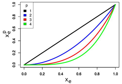
Figure 7.

Evacuation Process work.

10. Use case diagram

11. Conclusion

The methodology that has been used is considered to be simple and effective for the topology optimization problems especially the problems that need to reduce optimization over the volume constrains where it evaluates the structure frequently and demands hundreds of frequents and that is less 5% than the evolutionary algorithms. On the other hand, restricting the SIMP algorithm with a certain number of frequents might not give it the freedom to reach the optimal solution so that the user should be careful how to implement the variables of the algorithm.

References

- 1.
Nocedal J, Wright SJ. Numerical Optimization. 2nd ed. Springer; 2006. Available from: https://link.springer.com/book/10.1007/978-0-387-40065-5 - 2.
Pena SIV, Rionda SB. Topology Optimization Algorithms for the Solution of Compliance and Volume Problems in 2D. Mexico: A.C. Guanajuato; 2016. p. 24 - 3.
Botello S, Esqueda H, Gomez F, Moreles M, Onate E. Modulo de aplicaciones del metodo de los elementos finitos mefi 1.0, chapter manual teorico. CIMAT & CIMNE; 2004. pp. 6-69. Available from: https://cimat.repositorioinstitucional.mx/jspui/bitstream/1008/523/1/TE%20605.pdf - 4.
OC Zienkiewicz, RL Taylor, and JZ Zhu. The Finite Element Method: Its Basis and Fundamentals. 2005. Available from: https://www.researchgate.net/publication/334974685_State_of_the_art_of_generative_design_and_topology_optimization_and_potential_research_needs - 5.
Bendsøe MP. Optimal shape design as a material distribution problem. Structural Optimization. 1989; 1 (4):193-202 - 6.
Pena SIV, Rionda SB. Topology Optimization Algorithms for the Solution of Compliance and Volume Problems in 2D. Mexico: A.C. Guanajuato; 2016. pp. 4-6 - 7.
Tyflopoulos E, Flem DT, Steinert M, Olsen A. State of the Art of Generative Design and Topology Optimization and Potential Research Needs. Linköping, Sweden; 2018. pp. 6-8 - 8.
Rozvany GIN. Aims, scope, methods, history and unified terminology of computeraided topology optimization in structural mechanics. Structural and Multidisciplinary Optimization. 2001; 21 (2):90-108 - 9.
Zhou M, Rozvany GIN. The Coc Algorithm .2. Topological, Geometrical and Generalized Shape Optimization. Computer Methods in Applied Mechanics and Engineering. 1991; 89 (1–3):309-336 - 10.
Nha Chu D, Xie YM, Hira A, Steven GP. On various aspects of evolutionary structural optimization for problems with stiffness constraints. Finite Elements in Analysis and Design. 1997; 24 (4):197-212 - 11.
Stolpe M, Svanberg K. An alternative interpolation scheme for minimum compliance topology optimization. Structural and Multidisciplinary Optimization. 2001; 22 (2):116-124 - 12.
Deaton JD, Grandhi RV. A survey of structural and multidisciplinary continuum topology optimization: Post 2000. Structural and Multidisciplinary Optimization. 2014; 49 (1):1-38 - 13.
Luo Z, Chen L, Yang J, Zhang Y, Abdel-Malek K. Compliant mechanism design using multi-objective topology optimization scheme of continuum structures. Structural and Multidisciplinary Optimization. 2005; 30 (2):142-154 - 14.
Zhou M, Rozvany G. On the validity of ESO type methods in topology optimization. Structural and Multidisciplinary Optimization. 2001; 21 (1):80-83 - 15.
Xie YM, Steven GP. A simple evolutionary procedure for structural optimization. Computers & Structures. 1993; 49 (5):885-896 - 16.
Xie YM, Huang X. Recent developments in evolutionary structural optimization (ESO) for continuum structures. In: IOP Conference Series: Materials Science and Engineering. 2010. Available from: https://www.researchgate.net/publication/230941501_Recent_developments_in_evolutionary_structural_optimization_ESO_for_continuum_structures - 17.
Balamurugan R, Ramakrishnan CV, Singh N. Performance evaluation of a two stage adaptive genetic algorithm (tsaga) in structural topology optimization. Applied Soft Computing. 2008; 8 (4):1607-1624 - 18.
Bureerat S, Limtragool J. Performance enhancement of evolutionary search for structural topology optimisation. Finite Elements in Analysis and Design. 2006; 42 (6):547-566 - 19.
Hansel W, Treptow A, Becker W, Freisleben B. A heuristic and a genetic topology optimization algorithm for weight- minimal laminate structures. Composite Structures. 2002; 58 (2):287-294