Application of Polynomials in Coding of Digital Data

Abstract

Communication of information is nowadays ubiquitous in the form of words, pictures and sound that require digital conversion into binary coded signals for transmission due to the requirement of electronic circuitry of the implementing devices and machines. In a subtle way, polynomials play a very deep, important role in generating such codes without errors and distortion over long multiple pathways. This chapter surveys the very basics of such polynomials-based coding for easy grasp in the realization of such a complicated technologically important task. The coding is done in terms of just 0 and 1 that entails use of the algebra of finite Galois fields, using polynomial rings in particular. Even though more than six decades have passed since the foundations of the subject of the theory of coding were laid, the interest in the subject has not diminished as is apparent from the continued appearance of books on the subject. Beginning with the introduction of the ASCII codification of alpha-numeric and other symbols developed for early generation computers, this article proceeds with the application of algebraic methods of coding of linear block codes and the polynomials-based cyclic coding, leading to the development of the BCH and the Reed–Solomon codes, widely used in practices.

1. Introduction

Communication from a “source” to a “receiver” forms a vast buzz of activity over the entire globe. Physically, it is carried out as digital signals transmitted via different pathways such as light pulses through fiber-optic cables and radiowaves through air and even over the outer space. The digital signals are created in bits of pulses by electronic circuitry that work on the principle of (nearly) 0 and + 5 volts (Leach et al. [1], p. 3). A handy mathematical representation of the two voltages is just the set of two elements {0, 1}. An information thus consists of a string of 0’s and 1’s carried optically or electromagnetically through air or outer space as the case may be. The physical channel of information transmission is naturally noisy that was treated mathematically by Claude Shannon in a seminal paper [2] entitled “A mathematical theory of communication”, showing that in such noisy channel, there is a number called channel capacity such that reliable communication is achieved at any rate below the channel capacity by proper encoding and decoding techniques of any information. This paper marked the beginning of the subject of Coding Theory for encoding and decoding of information through the maze of channels.

In its widespread usage, information can be literal or numeric. It can also be audio or video, all encoded in $\left\{0,1\right\}$ bits. Moreover, special encoding and decoding is required for compression of the data at the very source to reduce the volume, storage on hard disks and encryption and decryption to maintain security of the data to be transmitted. The subject is therefore vast, and the mathematics involved is very special over the two numbers 0 an 1, studied in Abstract Algebra as a very special example of a finite field. However, according to Richard Hamming, a pioneer of the subject, “Mathematics is an interesting intellectual sport but it should not be allowed to stand in the way of obtaining sensible information about physical processes”. In that spirit, this article is aimed to provide just the flavor of introducing the use of polynomials over the $\left\{0,1\right\}$ field for developing a few practical methods of coding. No attempt is made to describe the corresponding methods of decoding, keeping in view the scope of this article. Detailed account of the subject and other methods of coding not treated here can be found in the texts by Bose [3], Kythe and Kythe [4], Roth [5], Moon [6], Ling and Xing [7], Blahut [8], Gathen and Gerhard [9], Proakis and Salehi [10], Adámek [11], and Lin and Costello [12]. All of these texts deal with polynomials over finite Galois fields to varying degrees of detail for the development of important codes like the practically important cyclic codes introduced by Prange [13], the BCH codes discovered by Bose, Ray-Chaudhuri [14] and independently by Hocqenghem [15], and the RS codes developed by Reed and Solomon [16]. The texts cited above also describe in detail, decoding methods of coded messages by a receiver, using special polynomials called syndromes. Besides the polynomials-based coding methods, the texts also give accounts of further development of codes with memory of past code words (convolutional coding) and codes for modulation of data transmission. Information theoretic probabilistic uncertainties of channelizing data transmission are also discussed in these texts to considerable extent. The list of texts is indicative of the continued interest in the topic of digital coding even now, ever since the appearance of the paper by Shannon. In what follows, Sections 2, 3, and 4 may be considered as preparatory coding methods before the appearance of polynomials over finite fields.

2. Coding

Transmission of a message of an information from a source to a destination is broadly classified into two categories: source coding of the message and channel coding for transmission through a channel. Both the types of coding are done mostly in terms of bits 0 and 1, because of the requirement of electronic implementation. Errors may occur at the source itself as well as in the transmission channel, and both of them require rectification in the transmitted message. The coding must be such that it can be uniquely decoded.

As an example of source coding, suppose that there is a message consisting of decimal numbers 0, 1, 2, 3, 4, ..... and alphabets A, B, C, D, ...... The first list can be bit converted by striking off the numbers 2, 3, ....., and 9. So that the binary code of 0, 1, 2, 3, 4, ..... becomes 0, 1, 10, 11, 100, ...... Coding a moderately large decimal number would be prohibitively very large and may not be uniquely decodable. For instance, the message 1011 could be decoded as 23 or 51 or 211. Giving a place value to the bits in the list as in the case of decimal numbers, a binary number listed as $a_0{a}_1{a}_2{a}_3\cdots$ can, however, be uniquely converted to its decimal equivalent by the polynomial expression

$${\left(a_0{a}_1{a}_2{a}_3\cdots \right)}_2={\left(\cdots \cdots a_3\times 2^3+a_2\times 2^2+a_1\times 2^1+a_0\times 2^0\right)}_{10}$$E1

where the suffixes 2 and 10 on the two sides of Eq. (1) indicate the concerned number to be binary or decimal as bases. Thus, the decimal equivalent of the binary

$$1011=1\times 2^3+0\times 2^2+1\times 2^1+1\times 2^0=8+0+2+1=11$$E2

But such a method is not applicable in the case of the alphabets A, B, C, D,......

Electronic hardware considerations on the other hand are realized for unique decoding using linear block codes, in which every numeral and alphabet is written in fixed length block of bits called word. In this respect the ASCII code of seven bits is important. For succinct coding, octal codes are used, in which the base is 8 consisting of the numbers 0, 1, 2, 3, 4, 5, 6, and 7 striking off the decimals 8 and 9. It can be easily verified that the octal digits can be represented by blocks of 3 bits as the two bits can be permuted in $2^3=8$

Octal digits	0	1	2	3	4	5	6	7
Binary blocks	000	001	010	011	100	101	110	111

The seven places of an ASCII word can be filled in $2^7=128$ ways by the two bits 0 and 1. Accordingly 128 symbols, alphanumeric or any other can be bit coded. A very short list of ASCII words is presented below:

0	1	2	3	A	B	C	$<$	=	$>$
$0{\left(60\right)}_8$	$0{\left(61\right)}_8$	$0{\left(62\right)}_8$	$0{\left(63\right)}_8$	$1{\left(01\right)}_8$	$1{\left(02\right)}_8$	$1{\left(03\right)}_8$	$0{\left(74\right)}_8$	$0{\left(75\right)}_8$	$0{\left(76\right)}_8$

A full table of the code is given in Adámek [8], p.10. In practice one additional bit place is kept with every ASCII word as a check, so that the word length is actually 8. An 8 bit word is called a byte. A computer usually uses a word length of 4 bytes or 32 bits. For representation in such long length, a base of 16 = $2^4$ bits is used to represent each symbol by 4 bits. Such coding is called hexadecimal represented by the 16 symbols 0, 1, 2,....., 9, A, B, C, D, E, F.

Audio and video information are continuous analog information. Such signals are sampled (see Leach et al. [1], p. 3) at small time or space–time intervals and are thus rendered discrete to generate digital data and suitably coded in bits. Foe instance, the basic colors of red, green, and blue are coded as $\#$FF0000, $\#$00FF00, and $\#$0000FF, respectively, where the code of the symbol $\#$ is $0{\left(43\right)}_8$. The respective color codes of white and black are $\#$FFFFFF and $\#$000000.

3. Algebraic formulation

A digital Code C is a sequence of words constituted of string of bits of some fixed length $n$. A code word $C$ can therefore be considered as an $n-$vector denoted as $\mathbf{a}=a_0{a}_1{a}_2\cdots a_{n-1}$ in which the elements $a_0,a_1,a_2,\cdots ,a_{n-1}\in \left(0,1\right)$. The commas separating the elements of a are dropped as unwanted symbol to form the block of bits. A code word of $C$ usually carries the message bits and some extra bits for detection of errors and their correction. This is necessary even though the loading time of bits increases to some extent. If the message consists of $k$ bits, and $n-k$ bits for error detection and correction, then it is called an $\left(n,k\right)$ code. Evidently by permutation, the number of messages in C that can be formed is $2^k$. As an example the $\left(7,4\right)$ code of three words

$$100001101001010010110$$

with the last three bits 011, 101, 110 of each message word represents the decimal number 842 according to the 4 bit hexadecimal representation of the three decimal digits.

A code $C$ when transmitted through a channel may contain some error and transmitted as $b_0{b}_1{b}_2\cdot b_{n-1}$ instead of the actual code $a_0{a}_1{a}_2\cdots a_{n-1}$. For error detection and correction, the following definition named after Richard Hamming [17] is introduced to keep the code words to be as wide apart as possible.

Definition (Hamming distance). Given two words $\mathbf{a}=a_0{a}_1{a}_2\cdots a_{n-1}$and $\mathbf{b}=b_0{b}_1{b}_2\cdots b_{n-1}$ their distance $d\left(\mathbf{a},\mathbf{b}\right)$ is defined as the number of positions in which a and b differ. Thus,

$$d\left(\mathbf{a},\mathbf{b}\right)=\text{number\hspace{0.17em}of\hspace{0.17em}indices\hspace{0.17em}if\hspace{0.17em}or\hspace{0.17em}which}{a}_i\ne b_i,\left(i=0,1,2,\cdots ,n-1\right)$$E3

As an example consider three words $\mathbf{x}=1000011$, $\mathbf{y}=0100101$, and $\mathbf{z}=0010110$ of the preceding example, then $d\left(\mathbf{x}.\mathbf{y}\right)=d\left(\mathbf{y},\mathbf{z}\right)=d\left(\mathbf{z},\mathbf{x}\right)=4$. But x and y as before and $\mathbf{z}=1100110$, one gets $d(\mathbf{x},\mathbf{y}=4$, $d\left(\mathbf{y},\mathbf{z}\right)=d\left(\mathbf{z},\mathbf{x}\right)=3$. The 4 bit message of the example in decimals is $x=8,y=4,z=2$ while $z=C$ (in Hex) or decimal 12, in the second case. It may be observed that $d\left(\mathbf{x},\mathbf{y}\right)\le d\left(\mathbf{y},\mathbf{z}\right)+d\left(\mathbf{z},\mathbf{x}\right)$ and $d\left(\mathbf{z},\mathbf{x}\right)\le d\left(\mathbf{x},\mathbf{y}\right)+d\left(\mathbf{y},\mathbf{z}\right)$. In general, it can easily be shown that the Hamming distance $d\left(\mathbf{a},\mathbf{b}\right)$ is a metric on the set of words of length $n$ satisfying the triangle inequality (Adámek [11], p. 46), as demonstrated in the example.

The definition of Hamming distance is useful for detection of errors in the following manner. A block code $C$ is said to detect $t$ errors provided that for each code word a and each word b obtained from a by corrupting $1,2,\cdots ,t$ symbols b is not a code word.

Definition. The minimum distance $d\left(C\right)$ of a code $C$ is the smallest Hamming distance of two distinct code words of the code $C$, that is,

$$d\left(C\right)=min\left\{d\left(\mathbf{a},\mathbf{b}\right)|\mathbf{a},\mathbf{b}\mathrm{are}\text{word}sinC\text{and}\mathbf{a}\ne \mathbf{b}\right\}$$E4

For example suppose that $C=\left[100001101001010010110\right],d\left(C\right)=4$ and for $=\left[100001101001011100110\right],d\left(C\right)=3$. The following proposition deals with the question of detection of errors in a code.

Proposition 1. A code $C$ detects $t$ errors if and only if $d\left(C\right)>t$.

Proof. If $d\left(C\right)\le t$, then $C$ does not detect $t$ errors. In fact, let a, a’ be correct and received code words with $d\left(\mathbf{a},{\mathbf{a}}^{\prime }\right)=d\left(C\right)$. Then $d\left(\mathbf{a},{\mathbf{a}}^{\prime }\right)\le t$, so the error which changes the original code a to the received word a’ escapes undetected. On the other hand, if $d\left(C\right)>t$, then $C$ detects $t$ errors. For, by definition, $1\le d\left(\mathbf{a},{\mathbf{a}}^{\prime }\right)\le t$. Then a’ can not be a code word since $d\left(C\right)\le d\left(\mathbf{a},{\mathbf{a}}^{\prime }\right)\le t$.

Regarding correction of codes, let a’ be the word obtained by corrupting $1,2,\cdots ,t$ bits of the code word a, then the Hamming distance $d\left(\mathbf{a},{\mathbf{a}}^{\prime }\right)$ is strictly smaller than that between a’ and any other code word b, that is, $d\left(\mathbf{a},{\mathbf{a}}^{\prime }\right)<d\left(\mathbf{b},{\mathbf{a}}^{\prime }\right)$. This leads to the following:

Proposition 2. A code $C$ corrects $t$ errors if and only if $d\left(C\right)\ge 2t+1$.

Proof. Let $d\left(C\right)\ge 2t+1>2t$, where $d\left(\mathbf{a},{\mathbf{a}}^{\prime }\right)\le t$. Hence for any other code word $\mathbf{b}\ne \mathbf{a}:d\left(\mathbf{a},\mathbf{b}\right)\ge d\left(C\right)>2t$, and by the triangle inequality

$$d\left(\mathbf{a},{\mathbf{a}}^{\prime }\right)+d\left({\mathbf{a}}^{\prime },\mathbf{b}\right)\ge d\left(\mathbf{a},\mathbf{b}\right)>2t$$

Hence,

$$d\left({\mathbf{a}}^{\prime },\mathbf{b}\right)>2t-d\left(\mathbf{a},{\mathbf{a}}^{\prime }\right)\ge 2t-t=t\ge d\left(\mathbf{a},{\mathbf{a}}^{\prime }\right)$$

which means that $C$ is a $t$ error correcting code.

The proof of the converse is more complicated (Adámek [11], p/49), but the proposition has a simple geometric interpretation. Every code word of $C$ can be thought of as a point in the $n$-dimensional vector space. Hence, every code word of Hamming distance of $t$ or less would lie within a sphere centered at the code word with a radius of $t$. Hence, $d\left(C\right)>2t$ implies that none of these spheres intersect. Any received vector a’ of a within a specific sphere will be closed to its center a and thus decodable correctly, being the nearest neighbor.

4. Linear block codes: generator matrix

As one is dealing here with only two numbers 0 and 1, the arithmetic over the two bits have to be redefined. For this purpose, congruence of two numbers from the Theory of Numbers is employed. For a given integer $n>1$, called modulus, two integers $a$ and $b$ are said to be congruent modulo m if $\left(a-b\right)/m$ = an integer and one writes a $\cong b$ (mod $m$). Thus, for $m=2$

$$2\cong 0\left(\mathit{mod}2\right),3\cong 1\left(\mathit{mod}2\right),4\cong 0\left(\mathit{mod}2\right),5\cong 1\left(\mathit{mod}2\right),\mathit{etc}.$$E5

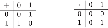
Thus, addition and multiplication of the bits 0 and 1 adopting modulo 2 congruence is conveniently represented in tabular form as:

This particular arithmetic is very useful in the development of very useful codes. One is by use of matrices. In the table for addition, it is noteworthy that $1+1=0$ so that $-1=1$.

A message of length $k$ in a binary $\left(n,k\right)$ block $C$ can be formed by permutation of 0 and 1 in $2^k$ ways. In practice $k$ is large, and so the dictionary of words becomes very large. For abbreviation let it be assumed that the codewords belong to $k$-dimensional linear vector space of $n$-vectors. The $k$ basis vectors of the $n$-vectors can then be employed to write any code word of $C$ by a linear combination of the basis vectors. This means that if ${\mathbf{e}}_{\mathbf{1}},{\mathbf{e}}_{\mathbf{2}},\cdots ,{\mathbf{e}}_{\mathbf{k}}$ are the (unit) basis vectors, then every code word a can be written as a linear combination

$$\mathbf{a}=\sum _{i=1}^k{c}_i{\mathbf{e}}_{\mathbf{i}}$$E6

for a unique $k$-tuple of scalars $c_i$. In other words, $c_1{c}_2\cdots c_k$ determine a unique code word. Eq. (6) can be written in matrix notation as

$$\mathbf{a}=\mathbf{c}\cdot \mathbf{G}$$E7

where

$$\mathbf{G}={\left[{\mathbf{e}}_{\mathbf{1}}{\mathbf{e}}_{\mathbf{2}}\cdots {\mathbf{e}}_{\mathbf{k}}\right]}^T$$E8

G is called the generator matrix of the code $C$. Evidently it is much more convenient to store G in the memory for generating any code word. For example, Adámek [11], p.72, Kythe and Kythe [4], p.76) consider the Hamming (7, 4) of $2^4=16$ code words as under:

Code word	Code word
0000 000	0110 011
1000 011	0101 010
0100 101	0011 001
0010 110	1110 000
0001 111	1101 001
1100 110	1011 010
1010 101	0111 100
1001 100	1111 111

employed by many authors for illustrative purposes of the coding methods, as the actual code words in practice are very long for unveiling the special features of the different methods of coding. The generator matrix of the code is

$$\mathbf{G}=\left[\begin{array}{ccccccc}1& 0& 0& 0& 0& 1& 1\\ 0& 1& 0& 0& 1& ,0& 1\\ 0& 0& 1& 0& 1& 1& 0\\ 0& 0& 0& 1& 1& 1& 1\end{array}\right]$$E9

Every code word of the code can be generated from it by a linear combination of the rows. For instance, the second code word is generated by taking $c_1=1,c_2=c_3=c_4=0$ and the third by taking $c_1=0,c_2=1,c_3=c_4=0$, etc.

By a change of basis the generator matrix changes. The most systematic way is to send the message $c_0{c}_1\cdots c_{k-1}$ by sending it as $c_0{c}_1\cdots c_{k-1}{d}_k\cdots d_{n-1}$ whose generator matrix is

$$\mathbf{G}=\left[\mathbf{I}|\mathbf{P}\right]$$E10

where I is the $k\times k$ identity (unit) matrix, and P is a $k\times \left(n-k\right)$ matrix called the parity matrix. In the above example, the generator matrix is in the systematic form with

$${\mathbf{P}}^{\mathbf{T}}=\left[\begin{array}{cccc}0& 1& 1& 1\\ 1& 0& 1& 1\\ 1& 1& 0& 1\end{array}\right]$$E11

Definition. An $\left(n,k\right)$ code $C$ with a generator $\mathbf{G}=\left[\mathbf{I}|\mathbf{P}\right]$ in systematic form is defined to have a parity check matrix $\mathbf{H}=\left[-\mathbf{P}|{\mathbf{I}}^{\prime }\right]$ where I′ is the identity matrix of dimension $n-k$.

From the above definition, it immediately follows that.

Proposition 3. The matrix ${\mathbf{H}}^{\mathbf{T}}$ is orthogonal to G.

Proof. ${\mathbf{GH}}^{\mathbf{T}}=\left[\mathbf{I}|\mathbf{P}\right]\left[\begin{array}{c}-\mathbf{P}\\ {\mathbf{I}}^{’}\end{array}\right]=-\mathbf{P}+\mathbf{P}=0$

This relation can be checked for the Hamming $\left(7,4\right)$ code keeping in mind the modulo-2 arithmetic for which $1+1=0$. This means that G is a correct generator of the $\left(7,4\right)$ code.

If an incorrect code word is transmitted which does not make G satisfy the condition ${\mathbf{GH}}^{\mathbf{T}}=0$, then that word does not belong to $C$, and the error is detected. In this way, the parity matrix helps detect errors.

In general, one has the Hamming codes [17] having the properties:

$$\begin{array}{l}\text{Block Length}:n=2^m-1\\ \text{Message Length}:k=2^m-m-1\end{array}$$

then it can be shown that the minimum distance of such codes is 3, and therefore, a Hamming code corrects a single error according to Proposition 2.

5. Finite fields

The modulo arithmetic over the elements of a finite set is particularly useful for algebraically extending further development of codes by introducing the definition of fields. As is well known, a field $F$ is a set of elements $\left\{0,1,a,b,c,\cdots \right\}$ over which two closed operations ${}^{`}{+}^{\prime }$ (addition) and ${}^{`}{\cdot }^{\prime }$ (multiplication) can be applied which satisfy the commutative, associative, and the distributive laws. For a nonzero element $a$, it is also assumed that a multiplicative inverse $a^{-1}\in F$exists such that $a\cdot a^{-1}=1.$. Usually one write $a\cdot b$ simply as $ab$. If in a set $F$ the multiplicative inverse does not exist, then it is called a Ring. If the number of elements of $F$ is finite, it is called a finite field. It is easy to verify that the field $F\left(2\right)$ of the bit set $\left\{0,1\right\}$ satisfying the mod 2 arithmetic is a finite field. However the set of all decimal integers $Z=\left\{0,\pm 1,\pm 2,\cdots \right\}$ forms an infinite integer ring. Similarly, the set of all polynomials $F\left(x\right)=\left\{a_0+a_{1}x+\cdots +a_n{x}^n:a_i\in F,n\ge 0\right\}$ also forms a polynomial ring.

Proposition 4. For every (decimal) prime $p$, $Z_p$ is a field.

Proof. Since $Z_p$ is a ring as noted earlier for $Z$ it is only required to prove that every element $i=1,2,\cdots ,p-1$ possesses an inverse. Firstly, $i=1$ has an inverse element $i^{-1}=1$. Secondly, suppose that for $i>1$ all the inverse elements $1^{-1},2^{-1},\cdots ,{\left(i-1\right)}^{-1}$ exist. Now perform the integer division $p/i$, denoting the quotient by $q\ne 0$ and the remainder by $r$; then one has

$$p=qi+r$$E12

Now, as $p$ is next to the last element $p-1\in Z_p$, so that in modulo $p$ arithmetic $p\cong 0$, and Eq. (13) means that

$$-r=q\cdot i=i\cdot q$$E13

Since $q\ne 0$ and $i$ lie between 2 and $p-1$, it follows that $r\ne 0$ so that $r^{-1}$ exists and $i=-q^{-1}\cdot r$. It follows that

$$i\cdot \left(-q\cdot r^{-1}\right)=-\left(i\cdot q\right)\cdot r^{-1}=-\left(-r\right)\cdot r^{-1}=1$$E14

which means that $i^{-1}$ exists and is equal to $-q\cdot r^{-1}$, and the proposition is proved by induction.

The above proposition shows that a number of finite fields exist, viz. $Z_2,Z_3,Z_5,Z_7,\cdots$. Of particular interest here is the field $Z_2$ which will be written as $\mathit{GF}\left(2\right)$ and its extension $\mathit{GF}\left(2^m\right)$ over the elements $\left\{0,1,\alpha ,{\alpha }^2,\cdots ,{\alpha }^{2^m}-1\right\}$ which is called the Galois field named after Éveriste Galois (CE 1811 – 1832), who earned fame in his teen age to die early in a gun dual to pass into the history of stellar mathematicians. The extension is based on the treatment of polynomials over the binary field.

6. Binary field polynomials

Consider calculation with polynomials whose coefficients are the binary bits $\left\{0,1\right\}$ of $\mathit{GF}\left(2\right)$. A polynomial $f\left(x\right)$ with one variable $x$ and binary coefficients is of the form

$$f\left(x\right)=a_0+a_{1}x+a_2{x}^2+\cdots +a_n{x}^n$$E15

where $a_i==0$ or 1 for $0\le i\le n$. If $a_n=1$, the polynomial is called monic of degree $n$. The variable is kept indeterminate and has only a formal algebraic role in coding.The polynomials of degree 1 over $\mathit{GF}\left(2\right)$ are evidently $x$ and $1+x$. Similarly, the polynomials of degree 2 are $x^2$, $1+x^2$, $x+x^2$, and $1+x+x^2$ and so on. In general, there are $2^n$ polynomials over $\mathit{GF}\left(2\right)$ with degree $n$.

Polynomials over Galois field $\mathit{GF}\left(2\right)$ can be added (or subtracted), multiplied, and divided in the usual way of treating real and complex valued polynomials.. Let

$$g\left(x\right)=b_0+b_{1}x+b_2{x}^2+\cdots ,b_m{x}^m$$E16

be another polynomial over $\mathit{GF}\left(2\right)$, where $m\le n$. Then, $f\left(x\right)$ and $g\left(x\right)$ are added by simply adding the coefficients of the same power of $x$ in $f\left(x\right)$ and $g\left(x\right)$:

$$f\left(x\right)+g\left(x\right)=\left(a_0+b_0\right)+\left(a_1+b_1\right)x+\cdots +\left(a_m+b_m\right)x^m+a_{m+1}{x}^{m+1}+\cdots a_n{x}^n$$E17

where $a_i+b_i$ is carried out in modulo-2 addition. For example, let $\varphi \left(x\right)=1+x+x^3+x^5$ and $\psi \left(x\right)=1+x+x^2+x^3+x^4+x^6$, then

$$\varphi \left(x\right)+\psi \left(x\right)=\left(1+1\right)+x+x^2+\left(1+1\right)x^3+x^4+x^5+x^6=x+x^2+x^4+x^5+x^6$$E18

as $1+1=0$. Similarly, when $f\left(x\right)$ is multiplied to $g\left(x\right)$, the following product is obtained

$$\begin{array}{l}{c}_0=a_0{b}_0\\ c_1=a_0{b}_1+a_1{b}_0\\ c_2=a_0{b}_2+a_1{b}_1+a_2{b}_0\\ ⋮\\ c_i=a_0{b}_i+a_1{b}_{i-1}+a_2{b}_{i-2}+\cdots +a_i{b}_0\\ ⋮\\ c_{n+m}=a_n{b}_m\end{array}$$E19

the multiplication and addition of the coefficients being in modulo-2. As a result, the polynomials $\varphi \left(x\right)$ and $\psi \left(x\right)$ satisfy the commutative, associative, and the distributive properties of addition and multiplication.

The division of $f\left(x\right)$ by $g\left(x\right)$ of nonzero degree can also be defined in the usual way by the division algorithm, so that $f\left(x\right)/g\left(x\right)$ leaves a unique quotient $q\left(x\right)$ and a remainder $r\left(x\right)$ in $\mathit{GF}\left(2\right)$, that is

$$f\left(x\right)=q\left(x\right)g\left(x\right)+r\left(x\right)$$E20

As an example consider $\psi \left(x\right)/\varphi \left(x\right)$:

$$\begin{array}{l}{x}^5+x^3+x+1)x^6+x^4+x^3+x^2+1(x\\ \underset{¯}{x^6+x^4+x^2+x}\\ x^3+x+1\end{array}$$

noting that $-x=x$ in $\mathit{GF}\left(2\right)$. Hence, $q\left(x\right)=x$ and $r\left(x\right)=1+x+x^3$. It can be easily verified that

$$x^6+x^4+x^3+x^2+1=x\left(x^5+x^3+x+1\right)+x^3+x+1$$

If a polynomial $f\left(x\right)$ in $\mathit{GF}\left(2\right)$ vanishes for some value $a\in \left(0,1\right)$, then $a$ is called a zero of $f\left(x\right)$ as in the case of real and complex variables. If $f\left(x\right)$ has even number of terms such as in the case of the polynomial $\varphi \left(x\right)$, then it is exactly divisible by $x+1$ as $\varphi \left(1\right)=1+1+1+1=0$. A polynomial $p\left(x\right)$ over $\mathit{GF}\left(2\right)$ of degree $m$ is called irreducible over $\mathit{GF}\left(2\right)$ if $p\left(x\right)$ is not divisible by any polynomial over $\mathit{GF}\left(2\right)$ of degree less than $m$. Among the four polynomials of degree 2, viz. $x^2$, $x^2+x$, $x^2+1$, $x^2+x+1$, the first three are reducible, since they are divisible by $x$ or $x+1$. However, $x^2+x+1$ does not have $x=0$ or $1$ as zero and so is not divisible by $x$ or $x+1$. Thus, $x^2+x+1$ is an irreducible polynomial of degree 2. Similarly, $x^3+x+1$ and $x^4+x+1$ are irreducible polynomials of degree 3 and 4, respectively, over $\mathit{GF}\left(2\right)$. It can be proved in general that (Gathen and Gerhard [9]):

Proposition 5. The polynomial $x^{2^m-1}+1$ over $\mathit{GF}\left(2\right)$ is the product of all irreducible monic polynomials.

Example 1. It can be verified by multiplication of the factors on the right hand sides that.

If $m=2$, $x^3+1=\left(x^2+x+1\right)\left(x+1\right)$.

If $m=3$, $x^7+1=\left(x^3+x+1\right)\left(x^3+x^2+1\right)\left(x+1\right)$.

If $m=4$, $x^{15}+1=\left(x^4+x+1\right)\left(x^4+x^3+1\right)\left(x^4+x^3+x^2+x+1\right)\left(x+1\right)$, etc.

An irreducible polynomial $p\left(x\right)$ of degree $m$ is said to be primitive if $m$ is the smallest positive integer for which $p\left(x\right)$ divides $x^{2^m-1}+1$. It is not easy to identify a primitive polynomial because of difficulty in factorizing $x^{2^m-1}+1$. However, comprehensive tables have been prepared for them for reference purposes (Lin and Costello [9]). A very short table is presented below:

$m$	Primitive Polynomial
2	$1+x+x^2$
3	$1+x+x^3$
4	$1+x+x^4$
5	$1+x^2+x^5$
6	$1+x+x^6$
7	$1+x^3+x^7$
8	$1+x^2+x^3+x^4+x^8$
9	$1+x^4+x^9$
10	$1+x^3+x^{10}$

Finally, the following interesting property holds.

Proposition 6. For any $l\ge 0$, ${\left[f\left(x\right)\right]}^{2^l}=f\left(x^{2^l}\right)$.

Proof.

$$\begin{array}{l}{f}^2\left(x\right)={\left[a_0+\left(a_{1}x+a_2{x}^2+\cdots +a_n{x}^n\right)\right]}^2\\ =a_0^2+a_0\cdot \left(a_{1}x+a_2{x}^2+\cdots a_n{x}^n\right)+a_0\cdot \left(a_{1}x+a_2{x}^2+\cdots a_n{x}^n\right)\\ +{\left(a_{1}x+a_2{x}^2+\cdots +a_n{x}^n\right)}^2\\ =a_0^2+{\left(a_{1}x+a_2{x}^2+\cdots +a_n{x}^n\right)}^2\end{array}$$

as $1+1=0$. By similar repeated expansion, it follows that

$$f^2\left(x\right)=a_0^2+{\left(a_{1}x\right)}^2+{\left(a_2{x}^2\right)}^2+\cdots {\left(a_n{x}^n\right)}^2$$

Now since, $a_i=0$ or 1, $a_i^2=a_i$, so that

$$f^2\left(x\right)=a_0+a_1{x}^2+a_2{\left(x^2\right)}^2+\cdots +a_n{\left(x^n\right)}^2=f\left(x^2\right)$$

Squaring again one has $f^4\left(x\right)=f\left(x^4\right)$ and so on. Hence, the result for $l\ge 0$.

Corollary. If for an element $\beta$, $f\left(\beta \right)=0$, then $f\left({\beta }^{2^l}\right)=0$. The element ${\beta }^{2^l}$ is called a conjugate of $\beta$.

6.1 Construction of Galois field GF($2^m)$

The Galois field extension $\mathit{GF}\left(2^m\right)$ from that of $\mathit{GF}\left(2\right)=\left\{0,1\right\}$ is obtained by introducing a new element say $\alpha$, in addition to 0 and 1. Then, by definition of multiplication

$$\begin{array}{c}0\cdot \alpha =\alpha \cdot 0=0,1\cdot \alpha =\alpha \cdot 1=\alpha ;\\ {\alpha }^2=\alpha \cdot \alpha ,{\alpha }^3=\alpha \cdot \alpha \cdot \alpha ,\cdots ,{\alpha }^j=\alpha \cdot \alpha \cdots \alpha j\left(\text{times}\right)\end{array}$$E21

Thus, a set $F$ is created by “multiplication” as

$$F=\left\{0,1,\alpha ,{\alpha }^2,\cdots ,{\alpha }^j,\cdots \right\}$$E22

Next, a condition is put on $\alpha$ so that $F$ contains only $2^m$ elements and is closed under the multiplication “$\cdot$”. For this purpose, let $p\left(x\right)$ be a primitive polynomial of degree $m$ over $\mathit{GF}\left(2\right)$ such that $\alpha$ is a zero of $p\left(x\right)$, that is, $p\left(\alpha \right)=0$ over $\mathit{GF}\left(2^m\right)$. Since $p\left(x\right)$ divides $x^{2^m-1}+1$ exactly according to Proposition 5, one has

$$x^{2^m-1}+1=q\left(x\right)p\left(x\right)$$E23

where $q\left(x\right)$ is the quotient and zero the remainder. Hence, taking $x=\alpha$,

$${\alpha }^{2^m-1}+1=q\left(\alpha \right)p\left(\alpha \right)=q\left(\alpha \right)\cdot 0=0$$E24

So that by modulo-2 addition

$${\alpha }^{2^m-1}=1$$E25

terminating the sequence in Eq. (26) at ${\alpha }^{2^m-1}$. Thus, under the condition $p\left(\alpha \right)=0$, the set becomes a finite set $F^{\ast }$ consisting of the $2^m$ elements

$$F^{\ast }=\left\{0,1,\alpha ,{\alpha }^2,\cdots ,{\alpha }^{2^m-1}\right\}$$E26

The nonzero elements of $F^{\ast }$ are closed under the operation of multiplication. For proving this property, consider the product ${\alpha }^i\cdot {\alpha }^j={\alpha }^{i+j}$. If $i+j<2^m-1,{\alpha }^{i+j}\in F^{\ast }$. If $i+j\ge 2^m-1$, then writing $i+j=\left(2^{m-1}-1\right)+r$, where $0\le r<2^m-1$,

$${\alpha }^{i+j}={\alpha }^{2^m-1+r}=1\cdot {\alpha }^r={\alpha }^r$$E27

by Eq. (26), in which ${\alpha }^r$ is an element of $F^{\ast }$.

The nonzero elements of $F^{\ast }$ are also closed under the operation of addition. For this purpose, divide $x^i,\left(0\le i\le 2^m-1\right)$ by $p\left(x\right)$ the primitive polynomial of degree $n$, where $p\left(\alpha \right)=0$ as before; then for $0\le i<2^m-1$ one can write

$$x^i=q_i\left(x\right)p\left(x\right)+r_i\left(x\right)$$E28

in which $q_i\left(x\right)$ and $r_i\left(x\right)$ are quotient and remainder, respectively. The remainder $r_i\left(x\right)$ is a polynomial of degree $m-1$ or less over $\mathit{GF}\left(2\right)$ and hence is of the form

$$r_i\left(x\right)=r_{i0}+r_{i1}x+r_{i2}{x}^2+\cdots +r_{i,m-1}{x}^{m-1}$$E29

Hence, setting $x=\alpha$

$${\alpha }^i=r_{i0}+r_{i1}\alpha +r_{i2}{\alpha }^2+\cdots +r_{i,m-1}{\alpha }^{m-1}$$E30

Similarly if $0\le j<2^{m-1}$, ${\alpha }^j$ can be represented as a polynomial at most of degree $m-1$. Thus, ${\alpha }^i+{\alpha }^j$ would be a polynomial at most of degree $m-1$, and by addition of the two polynomials, the summand would be equal to some ${\alpha }^k$ where $0\le k<2^{m-1}$. This proves the assertion.

Example 2. As in Lin and Costello [12], p. 32, let $m=4$, so that $\mathit{GF}\left(2^4\right)=\left\{0,1,\alpha ,{\alpha }^2,{\alpha }^3,{\alpha }^4,{\alpha }^5,{\alpha }^6,{\alpha }^7,{\alpha }^8,{\alpha }^9,{\alpha }^{10},{\alpha }^{11},{\alpha }^{12},{\alpha }^{13},{\alpha }^{14}\right\}$. Its primitive polynomial over $\mathit{GF}\left(2\right)$ is $p\left(x\right)=1+x+x^4$, so that set $p\left(\alpha \right)=1+\alpha ++{\alpha }^4=0$, or adding $1+\alpha$ to the two sides of the equation ${\alpha }^4=1+\alpha$. Hence,

$$\begin{array}{c}{\alpha }^5=\alpha \cdot {\alpha }^4=\alpha \cdot \left(1+\alpha \right)=\alpha +{\alpha }^2,{\alpha }^6=\alpha \cdot \left(\alpha +{\alpha }^2\right)={\alpha }^2+{\alpha }^3,\\ {\alpha }^7={\alpha }^3+{\alpha }^4=1+\alpha +{\alpha }^3,{\alpha }^8=\alpha +{\alpha }^2+{\alpha }^4=1+{\alpha }^2,\mathit{etc}.\end{array}$$

The highest power of $\alpha$ is 3 in these elements and the 4-tubles form the block code words of length 4, which can be represented in the hexadecimal code as well:

Power representation	Polynomial representation	4-tuple representation	Hexadecimal
0	0	(0 0 0 0)	0
1	1	(1 0 0 0)	8
$\alpha$	$\alpha$	(0 1 0 0)	4
${\alpha }^2$	${\alpha }^2$	(0 0 1 0)	2
${\alpha }^3$	${\alpha }^3$	(0 0 0 1)	1
${\alpha }^4$	1+$\alpha$	(1 1 0 0)	C
${\alpha }^5$	$\alpha +{\alpha }^2$	(0 1 1 0)	6
${\alpha }^6$	${\alpha }^2+{\alpha }^3$	(0 0 1 1)	3
${\alpha }^7$	$1+\alpha +{\alpha }^3$	(1 1 0 1)	D
${\alpha }^8$	$1+{\alpha }^2$	(1 0 1 0)	A
${\alpha }^9$	$\alpha +{\alpha }^3$	(0 1 0 1)	5
${\alpha }^{10}$	$1+\alpha +{\alpha }^2$	(1 1 1 0)	E
${\alpha }^{11}$	$\alpha +{\alpha }^2+{\alpha }^3$	(0 1 1 1)	7
${\alpha }^{12}$	$1+\alpha +{\alpha }^2+{\alpha }^3$	(1 1 1 1)	F
${\alpha }^{13}$	$1+{\alpha }^2+{\alpha }^3$	(1 0 1 1)	B
${\alpha }^{14}$	$1+{\alpha }^3$	(1 0 0 1)	9

Proposition 7. The elements of $\mathit{GF}\left(2^m\right)$ form all the zeros of $x^{2^m}+x$.

Proof. The proposition obviously holds for the element 0. For a nonzero element $\beta \in \mathit{GF}\left(2^m\right)$ let, $\beta ={\alpha }^i$ then ${\beta }^{2^m-1}={\alpha }^{i\left(2^m-1\right)}={\left({\alpha }^{2^m-1}\right)}^i=1^i=1$ by Eq. (26). Hence, by modulo-2 addition one has ${\beta }^{2^m-1}+1=0$ or, ${\beta }^{2^m}+\beta =0$.

The next proposition determines the minimal polynomial corresponding to an element $\beta \in \mathit{GF}\left(2^m\right)$:

Proposition 8. If f $e$ is the smallest integer for which ${\beta }^{2^e}=\beta$, then the minimal polynomial $\varphi \left(x\right)$ corresponding to $\beta \in \mathit{GF}\left(2^m\right)$ is given by

$$\varphi \left(x\right)={\mathrm{\Pi }}_{i=0}^{e-1}\left(x+{\beta }^{2^i}\right)$$E31

Proof. Since $\beta$ is a zero of $\varphi \left(x\right)$, $\varphi \left(\beta \right)=0$. Hence, by the Corollary to Proposition 6, $\varphi \left({\beta }^{2^i}\right)=0$ which means that ${\beta }^{2^i}$ is also a zero of $\varphi \left(x\right)$. Hence, $\varphi \left(x\right)$ is the product of the factors $x+{\beta }^{2^i}$, provided that $i$ is one less than that makes ${\beta }^{2^i-1}=1$ or, ${\beta }^{2^i}=\beta$.

Example 3. For $\beta ={\alpha }^3\in \mathit{GF}\left(2^4\right)$, the conjugates of $\beta$ are ${\beta }^2={\alpha }^6,{\beta }^{2^2}={\alpha }^{12},{\beta }^{2^3}={\alpha }^{24}={\alpha }^9$. The minimal polynomial of $\beta$ is $\varphi \left(x\right)=\left(x+{\alpha }^3\right)\left(x+{\alpha }^6\right)(x+{\alpha }^{12}\left(x+{\alpha }^9\right)=\left(x^2+{\alpha }^{2}x+\alpha +{\alpha }^3\right)\left[x^2+\left(1+{\alpha }^2\right)x+{\alpha }^2+{\alpha }^3\right]=x^4+x^3+x+1$, using the table given above, with ${\alpha }^{15}=1$.The following table gives the minimal polynomials for all the powers of $\alpha$ (Adámek [11], p. 216):

Elements	Minimal Polynomial
0	x
1	x + 1
$\alpha ,{\alpha }^2,{\alpha }^4,{\alpha }^8$	$x^4+x+1$
${\alpha }^3,{\alpha }^6,{\alpha }^9,{\alpha }^{12}$	$x^4+x^3+x^2+1$
${\alpha }^5,{\alpha }^{10}$	$x^2+x+1$
${\alpha }^7,{\alpha }^{11},{\alpha }^{13},{\alpha }^{14}$	$x^4+x^3+1$

Thus, all the irreducible minimal polynomial factors of $x^{2^4-1}+1$ are obtained.

7. Cyclic codes

Cyclic codes introduced by Prange [13] form an important subclass of linear codes by the introduction of additional algebraic structure that a cyclic shift of a code word is also a code word. Thus, if in a code word $\mathbf{a}=\left(a_0,a_1,\cdots ,a_{n-1}\right)$ of a cyclic code, a shift of one place to the right is made a new word ${\mathbf{a}}^{\left(1\right)}=\left(a_{n-1},a_0,a_1,\cdots ,a_{n-2}\right)$ is formed. Similarly, a shift of $l$ places to the right is made, then the word

$${\mathbf{a}}^{\left(l\right)}=\left(a_{n-l},a_{n-l+1},\cdots ,a_{n-1},a_0,a_1,\cdots ,a_{n-l-1}\right)$$E32

is formed. It may be checked that the $\left(7,4\right)$ Hamming code noted after Eq. (8) is not a cyclic code.

The special algebraic properties of the cyclic codes are described by a polynomial representation formed by the component elements of a:

$$f\left(x\right)=a_0+a_{1}x+a_2{x}^2+\cdots +a_{n-1}{x}^{n-1}$$E33

where $x$ is indeterminate, and the degree is $n-1$ or less according to $a_{n-1}=1$ or 0. Here, the polynomial is called a code polynomial, and the code word ${\mathbf{a}}^l$ is represented by the polynomial

$$f^{\left(l\right)}\left(x\right)=\left(a_{n-l}+a_{n-l+1}x+\cdots +a_{n-1}{x}^{l-1}\right)+\left(a_0{x}^l+a_1{x}^{l+1}+\cdots +a_{n-l-1}{x}^{n-1}\right)$$E34

The polynomial $f^{\left(l\right)}\left(x\right)$ can be represented in a compact form.

Proposition 9. $f^{\left(l\right)}\left(x\right)=x^{l}f\left(x\right)(\mathit{mod}{x}^n+1$).

Proof.

$$\begin{array}{c}{x}^{l}f\left(x\right)=a_0{x}^l+a_1{x}^{l+1}+\cdots +a_{n-l-1}{x}^{n-1}+a_{n-l}{x}^n+\cdots +a_{n-1}{x}^{n+l-1}\\ =\left(a_{n-l}+a_{n-l+1}x+\cdots +a_{n-1}{x}^{l-1}\right)+a_0{x}^l+\cdots +a_{n-l-1}{x}^{n-1}\\ +a_{n-l}\left(x^n+1\right)+a_{n-l+1}x\left(x^n+1\right)+\cdots +a_{n-1}{x}^{l-1}\left(x^n+1\right)\\ =q\left(x\right)\left(x^n+1\right)+f^{\left(l\right)}\left(x\right)\end{array}$$E35

where $q(\left(x\right)=a_{n-l}+a_{n-l+1}x+\cdots +a_{n-1}{x}^{l-1}$, which proves the theorem.

In general, consider an $\left(n,k\right)$ cyclic code $C$ that possesses a code polynomial

$$g\left(x\right)=1+g_{1}x+g_{2}x+\cdots +g_{r-1}{x}^{r-1}+x^r$$E36

of minimum degree $r$ (such as $1+x+x^3$ in the above given example), then the polynomials $\mathit{xg}\left(x\right)=g^{\left(1\right)}\left(x\right),x^{2}g\left(x\right)=g^{\left(2\right)}\left(x\right),\cdots ,x^{n-r-1}g\left(x\right)=g^{\left(n-r-1\right)}\left(x\right)$ represent cyclic shifts of the code polynomial $g\left(x\right)$ that are code polynomials in $C$. Since $C$ is linear, a linear combination

$$\begin{array}{c}\psi \left(x\right)=b_{0}g\left(x\right)+b_1\mathit{xg}\left(x\right)+\cdots +b_{n-r-1}{x}^{n-r-1}g\left(x\right)\\ =\left(b_0+b_{1}x+\cdots +b_{n-r-1}{x}^{n-r-1}\right)g\left(x\right)\end{array}$$E37

is also a code polynomial with $b_i=0$ or 1 of degree $n-1$ or less. The number of such polynomials is $2^{n-r}$. However, there are $2^k$ code polynomials in $C$, so that $n-r=k$ or, $r=n-k$. Thus,

Proposition 10. In an $\left(n,k\right)$ cyclic code $C$, one unique code polynomial

$$g\left(x\right)=1+g_{1}x+g_2{x}^2+\cdots +g_{n-k-1}{x}^{n-k-1}+x^{n-k}$$E38

of degree $n-k$ called the generator polynomial yields every binary polynomial code of degree $n-1$ or less by multiplication with another polynomial of degree $k-1$.

From Eq. (39), one can find a generator polynomial from the following:

Proposition 11. The generator polynomial $g\left(x\right)$ of an $\left(n,k\right)$ cyclic code is a factor of $x^n+1$.

Proof. Multiplying $g\left(x\right)$ by $x^k$ in Eq.(39), one obtains a polynomial $x^{k}g\left(x\right)$ of degree $n$. Hence, according to Eq. (36)

$$x^{k}g\left(x\right)=\left(x^n+1\right)+g^{\left(k\right)}\left(x\right)$$E39

where $g^k\left(x\right)$ is the remainder, which is a polynomial obtained by $k$ cyclic shifts of the coefficients of $g\left(x\right)$. Hence, $g^{\left(k\right)}\left(x\right)$ is a multiple of $g\left(x\right)$, say $\psi \left(x\right)$ of degree $k$, viz. $g^{\left(k\right)}\left(x\right)=\psi \left(x\right)g\left(x\right)$. Thus,

$$x^n+1=\left\{x^k+\psi \left(x\right)\right\}g\left(x\right)$$E40

which completes the proof.

In practice where $n$ is large $x^n+1$ may have several factors of degree $n-k$ to describe cyclic codes. For example (Lin and Costello [12], p. 90)

$$x^7+1=\left(1+x\right)\left(1+x+x^3\right)\left(1+x^2+x^3\right)$$

in which either of the last two factors can be selected for a generator polynomial. In the example considered earlier, we selected $g\left(x\right)=1+x+x^3$. In practice, it is difficult to make a choice because of implementation difficulty. Nevertheless it is possible to form the generator matrix of a cyclic code and parity-check matrix for error detection and correction. Lin and Costello [9] give an excellent treatment of the whole topic.

8. The BCH codes

The Bose, Chaudhuri, Hocqenghem (BCH) [14, 15] codes form a large class of powerful random error-correcting codes (Lin and Costello [9]). It generalizes the Hamming code in the following manner:

$$\begin{array}{l}\text{Block length}:n=2^m-1\\ \text{Parity check bits}:n-k\le \mathit{mt}\\ \text{Minimum distance}:d\ge 2t+1\end{array}$$E41

where $m\ge 3$, and $t<2^{m-1}$.

This code is capable of correcting any combination of $t$ or fewer errors in a code word of length $n=2^m-1$ bits and is called a $t-$error$-$correcting code.The generator polynomial of the code $g\left(x\right)$ of length $2^m-1$ is the lowest degree polynomial over $\mathit{GF}\left(2\right)$ which has

$$\alpha ,{\alpha }^2,{\alpha }^3,\cdots ,{\alpha }^{2t}$$E42

as its zeros, that is to say, $g\left({\alpha }^i\right)=0$ for $1\le i\le 2t$. It follows from the Corollary to Proposition 6 that the conjugates of the zeros $\alpha ,{\alpha }^2,{\alpha }^3,\cdots ,{\alpha }^{2t}$ are also zeros of $g\left(x\right)$. If ${\varphi }_i\left(x\right)$ is the minimal polynomial of ${\alpha }^i$, then $g\left(x\right)$ must be the lowest common multiple (LCM) of ${\varphi }_1\left(x\right),{\varphi }_2\left(x\right),\cdots {\varphi }_{2t}\left(x\right)$, that is

$$g\left(x\right)=\mathrm{LCM}\left\{{\varphi }_1\left(x\right),{\varphi }_2\left(x\right),\cdots ,{\varphi }_{2t}\left(x\right)\right\}$$E43

Now, if $i$ is an even integer, it can be written as $i=i^{\prime }{2}^l$ where $i^{\prime }$ is an odd number and $l\ge 1$. Then, for such $i$, ${\alpha }^i={\left({\alpha }^{i^{\prime }}\right)}^{2^l}$, which is conjugate of ${\alpha }^{i^{\prime }}$, and therefore, ${\alpha }^i$ and ${\alpha }^{i^{\prime }}$ have the same minimal polynomial, that is

$${\varphi }_i\left(x\right)={\varphi }_{i^{\prime }}\left(x\right)$$E44

Hence, every even power of $\alpha$ in the sequence (44) has the same minimal polynomial as some preceding odd power of $\alpha$ in the sequence. As a result, the generator $g\left(x\right)$ given by Eq. (44) reduces to

$$g\left(x\right)=\mathrm{LCM}\left\{{\varphi }_1\left(x\right),{\varphi }_3\left(x\right),\cdots ,{\varphi }_{2t-1}\left(x\right)\right\}$$E45

Since the degree of each minimal polynomial is $m$ or less, the degree of $g\left(x\right)$ is at most $\mathit{mt}$. This means that the number of parity-check bits $n-k$ of the code is at most $\mathit{mt}$. There is, however, no simple formula for enumerating the parity $n-k$ bits, but tables do exist for various values of $n,k,$ and $t$ (Lin and Costello [9]).

In the special case of single error correction for a $n=2^m-1$ long code word, $g\left(x\right)={\varphi }_1\left(x\right)$ which is a primitive polynomial of degree $2^m$. Thus, the single error correcting BCH code of length $2^m-1$ is a cyclic Hamming code.

Example 4. As in Lin and Costello [12], p. 149, let $\alpha$ be a primitive element of $\mathit{GF}\left(2^4\right)$ such that ${\alpha }^4+\alpha +1=0$. From Example 2,

$$\begin{array}{l}{\varphi }_1\left(x\right)=1+x+x^4\\ {\varphi }_3\left(x\right)=1+x+x^2+x^3+x^4\end{array}$$

Hence, the double error correcting BCH code of length $n=2^4-1=15$ is generated by

$$\begin{array}{c}g\left(x\right)=\mathrm{LCM}\left\{{\varphi }_1\left(x\right),{\varphi }_3\left(x\right)\right\}={\varphi }_1\left(x\right){\varphi }_3\left(x\right)\\ =\left(1+x+x^4\right)\left(1+x+x^2+x^3+x^4\right)\\ =1+x^4+x^6+x^7+x^8\end{array}$$

It is possible to construct the parity matrix $H$ of this code and is presented in Lin and Costello [9].

9. The RS codes

In the construction of BCH codes, the generator polynomials over $\mathit{GF}\left(2\right)$ were considered using the elements of the minimal polynomials over the extended field $\mathit{GF}\left(2^m\right)$. Since the minimal polynomial for an element $\beta$ also has all the conjugates of $\beta$ as the zeros of the minimal polynomial, the product of the minimal polynomials usually exceeds the number $2t$ of the specified zeros. In the Reed–Solomon (RS) codes [16], this situation is tackled by considering the extended $\mathit{GF}\left(2^m\right)$ as the starting point. An element $\beta \in \mathit{GF}\left(2^m\right)$ has obviously the minimal polynomial $x+\beta$. If $\beta ={\alpha }^i$ where $\alpha \in \mathit{GF}\left(2^m\right)$, the required generator $g\left(x\right)$ of degree $2t$ as in Eq. (46) becomes

$$g\left(x\right)=\left(x+{\alpha }^i\right)\left(x+{\alpha }^{i+1}\right)\cdots \left(x+{\alpha }^{i+2t-1}\right)$$E46

There are no extra zeros in $g\left(x\right)$ included by the conjugates of the minimal polynomial. So the degree of $g\left(x\right)$ is exactly $2t$. Thus, $n-k=2t$ for a RS code and the minimum distance by Proposition 2 is $d=2t+1=n-k+1$. Hence, an RS code is

$$\begin{array}{l}\text{Block\hspace{0.17em}length}:n=2^m-1\\ \text{Parity check bits}:n-k=2t\\ \text{Minimum distance}:d=n-k+1\end{array}$$E47

Example 5. Let $n=2^4-1=15$, and consider three error codes $\left(t=3\right)$ over $\mathit{GF}\left(2^4\right)$, having the primitive polynomial $p\left(x\right)=1+x+x^4$. Taking $i=1$ in Eq. (47) the required generator polynomial is

$$g\left(x\right)=\left(x+\alpha \right)\left(x+{\alpha }^2\right)\left(x+{\alpha }^3\right)(\left(x+{\alpha }^4\right)\left(x+{\alpha }^5\right)\left(x+{\alpha }^6\right)$$

where ${\alpha }^4=1+\alpha$, and ${\alpha }^{15}=1$. Thus simplifying, one gets the generator polynomial for the (15, 9) code over $\mathit{GF}\left(2^4\right)$ as

$$g\left(x\right)={\alpha }^6+{\alpha }^{9}x+{\alpha }^6{x}^2+{\alpha }^4{x}^3+{\alpha }^{14}{x}^4+{\alpha }^{10}{x}^5+x^6$$

The corresponding code word is ${\alpha }^6{\alpha }^9{\alpha }^6{\alpha }^4{\alpha }^{14}{\alpha }^{10}1$. Using the table of Example 2, one obtains the binary equivalent over $\mathit{GF}\left(2\right)$ as

$$0011010100111100100111101000$$

The length of the binary word is 28. This type of code is called derived binary code.

10. Conclusion

In this information age transmission of data is all pervasive due to immense development of electronic technology. In this general scenario, it is rarely recognized that the foundations of this information web were layed by “A mathematical theory of communication” propounded by Claude E. Shannon [2] that called for means of error-free transmission of information as digital data. This realization led to the creation of Theories of Coding by more mathematicians, pioneered by Richard W. Hamming [17] emphasizing that data need to be appropriately coded for realizing the objectives. As digital data consist of just two bits 0 and 1, special algebra were employed which were based on the algebra of finite fields. In this endeavor, several types of data coding have been discovered and put to practical use depending on the application. Some of the codes developed depend on polynomials over the binary field of 0 and 1; prominent among them being the BCH [14, 15] and the RS codes [16] that are widely used in practice. This chapter gives a simple mathematical preview of this type of code development and is intended for those who may be interested to further delve into the subject of coding of digital data.

Acknowledgments

The author is thankful to the SN Bose National Center for Basic Sciences for supporting this research, as also to the referees for their learned comments for the improvement in the presentation of this article.

Disclosures

There is no conflict of interests in the presented chapter.

Data availability

No data were generated or analyzed in the presented chapter.