Fitting Parametric Polynomials Based on Bézier Control Points

Abstract

This chapter provides an overview at fitting parametric polynomials with control points coefficients. These polynomials have several properties, including flexibility and stability. Bézier, B-spline, Nurb, and Bézier trigonometric polynomials are the most significant of these kinds. These fitting polynomials are offered in two dimensions (2D) and three dimensions (3D). This type of polynomial is useful for enhancing mathematical methods and models in a variety of domains, the most significant of which being interpolation and approximation. The utilization of parametric polynomials minimizes the number of steps in the solution, particularly in programming, as well as the fact that polynomials are dependent on control points. This implies having more choices when dealing with the generated curves and surfaces in order to produce the most accurate results in terms of errors. Furthermore, in practical applications such as the manufacture of automobile exterior constructions and the design of surfaces in various types of buildings, this kind of polynomial has absolute preference.

1. Introduction

Curve (or surface) fitting to a set of provided data points based on control points is a common and often performed activity in many areas of science and engineering, including machine vision, computer vision, reverse engineering, coordinate metrology, and computer-aided geometric design.

When fitting a collection of data points in two- and three-dimensional space, the shortest distance (which is also known as Euclidean distance, geometric distance, or orthogonal distance) between the curve (or surface) and the data points point has practical significance [1, 2, 3]. The fitting of a parametric curve or surface using this error measure is known as “orthogonal distance fitting” or “geometric fitting” [4, 5, 6, 7, 8, 9, 10, 11]. The geometric fitting issue is a nonlinear minimization problem that must be addressed iteratively, and it is widely acknowledged as an analytically and computationally challenging problem. There are two new methods for geometric fitting of functional curves and surfaces: [4, 6, 9, 11] for implicit curves and surfaces and [10, 12, 13] for parametric curves and surfaces. For a long time, the theoretical and computational problems in computing and decreasing geometric distances challenged the development of geometric fitting algorithms for functional curves/surfaces [6, 7]. Most data processing software programs use approximation measures of geometric distance to avoid the challenges associated with geometric fitting [8, 14, 15, 16, 17, 18]. Nonetheless, when highly accurate and reliable estimation of parameter estimation is required by applications, we have no choice but to use geometric distance as the error measure for functions based on control points fitting, despite the high computational cost and difficulties in developing geometric fitting algorithms. In fact, an international standard requires the use of the geometric error measure for testing data processing software for coordinate metrology [2].

Ameer et al. [19] developed a new Bézier polynomial with two form parameters based on new generalized Bernstein basis functions. Both Bernstein basis functions and Bézier polynomials have geometric features that are analogous to the classical Bernstein basis and Bézier curve, respectively. Using the described Bézier curves and surfaces as applications, several free-form curves may be represented.

Khan et al. [20] investigate weighted Lupaş post-quantum Bernstein blending functions and Bézier curves built using bases through $\left(p,q\right)$ integers. Because of their degree elevation qualities and the de Casteljau technique, quadratic weighted Lupaş post-quantum Bézier curves may represent conic sections in the two-dimensional plane. Compared to traditional rational Bézier curves, Lupaş q-Bézier curves, and weighted Lupaş q-Bézier curves, its generalization provides superior approximation and adaptability to a specific control point as well as a control polygon.

Özger [21] defined a new type of Bézier base using $\lambda$ shape parameters. He creates a new type of Schurer operator by defining new Bézier-Schurer bases.

Fitting parametric Bézier-like curves and surfaces in two- and three-dimensional space based on control points is the focus of this chapter.

2. Parametric polynomials

In computer graphics, we frequently need to draw many types of objects onto the screen. Objects are not always flat, and we must draw curves several times in order to depict an object. A curve is a collection of infinitely many points. Except for endpoints, each point has two neighbors. Curves are broadly classified into three types: explicit, implicit, and parametric. A curve can be created for the mathematical function $y=f\left(x\right)$, which gives an explicit representation of the curve. The explicit representation is not general since it cannot express vertical lines and is also single-valued. Normally, the function computes only one value of $y$ for each value of $x$.

The most basic practice for writing a curve equation is implicit representation, which combines all variables into one lengthy, non-linear equation, like as follows:

$$a{x}^3+b{y}^2+2\mathit{cxy}+2\mathit{dx}+2\mathit{ey}+f=0.$$E1

To compute the values and plot them on a graph in this representation, we must solve the complete non-linear equation.

Some interactions between two numbers or variables are so complex that we occasionally incorporate a third quantity or variable to simplify matters. This third number is known as a parameter. Instead of a single equation relating, say, $x$ and $y$, we have two, one related to the $x$ parameter and one relating to the $y$ parameter.

The parametric representation rewrites the equation into shorter, more readily solvable equations that transform the values of one variable into the values of the others:

$$x=a+\mathit{bt}+c{t}^2+d{t}^3$$E2

$$y=g+\mathit{ht}+j{t}^2+k{t}^3$$E3

The equations for $x$ and $y$ are straightforward when using this form. We just require a value for $t$, which is the point along the curve where we wish to compute $x$ and $y$. Parametric curves can be imagined as being drawn by a point passing through space. We can determine the $x$ and $y$ values of the moving point at any value of $t$. This is a critical issue since many tools depend on the notion of associating a parameter number with each point on the line. This relates to the curve’s $U$ dimension.

3. Bézier curves

An explicit Bézier curves is one for which the x-coordinates of the control points are evenly spaced between 0 and 1. A Bézier curve takes on the important special form

$$x=t$$E4

$$y=f\left(t\right)$$E5

or simply

$$y=f\left(x\right).$$E6

An explicit Bézier curves is sometimes called a non-parametric Bézier curve and it developed by A French engineer named Pierre Bézier to define the computer graphics curve. This function generates a Bézier curve, the form of which is specified by control points. The inner control points (points not on the curve) determine the form of the curve, whereas the end control points specify the endpoints of the curve.

An $n$th-degree of Bezier curve is depicted by the formula below.

$$P\left(t\right)=\sum _{a=0}^{\theta }{p}_a{B}_a^{\theta }\left(t\right),$$E7

where $t\in \left[0,1\right]$ is the parameter, $n$ is the degree of Bezier curve, and $p_a=\left(p_x^{\left(a\right)},p_y^{\left(a\right)}\right)$ are the control points.

The basis functions, are the parametric Bernstein polynomial of degree $\theta$ which are defined explicitly by

$$B_a^{\theta }\left(t\right)=\left(\genfrac{}{}{0pt}{}{\theta }{a}\right)t^a{\left(1-t\right)}^{\theta -a}$$E8

with $\left(\genfrac{}{}{0pt}{}{\theta }{a}\right)=\frac{\theta !}{a!\left(\theta -a\right)!}$ and $\theta \in Z^{+}$. Figure 1 shows a degree five explicit Bézier curve.

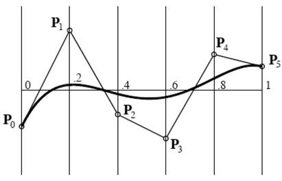
Figure 1.

Explicit Bézier curve.

Eq. (7) is alternatively parametrically expressed as

$$P\left(t\right)=\left(x\left(t\right),y\left(t\right)\right)$$E9

with

$$x\left(t\right)=\sum _{a=0}^{\theta }{p}_x^{\left(a\right)}{B}_a^{\theta }\left(t\right)$$E10

and

$$y\left(t\right)=\sum _{a=0}^{\theta }{p}_y^{\left(a\right)}{B}_a^{\theta }\left(t\right).$$E11

Several construction-based Bezier control points are used in this work to find interpolation polynomials.

4. Fitting Bézier polynomials

Approximation and interpolation approaches can be used to fit the curve (or surface). However, classical interpolation and interpolation with control points are the most extensively utilized approaches [22]. Control points, with the exception of the end control points, are points that do not appear on the curves, but they regulate the form of the curves (or surfaces). In other words, control points function like magnets.

4.1 Fast Bézier interpolator

Yau and Wang [23] suggested a Fast Bézier interpolator approach for generating control points to produce a local Bézier interpolating polynomial. In this approach, the data points were categorized according to their distribution. The values of two inner control points might be obtained by meeting the stated requirements for each set of data points. The arc was formed by intersecting line segments between data points and applying the angle criteria. The inaccuracy from matching the data points with the arc was then used to determine the curve in each segment. Nevertheless, the mathematical procedure for determining the value of two inner control points for each subinterval is time-consuming due to the numerous computations required.

Figure 2 is a chart of cubic Bezier curve-fitted continuous short blocks (CSBs), often known as $G_{01}$ blocks. $P_1-P_8$ and $P_9-P_n$ are curves made up of CSBs fitted by two cubic Bezier curves, respectively. The corner angles are $y_1$ and $y_2$. The lengths of the cubic Bezier curves are $L_1$ and $L_3$. $L_2$ denotes the length of a $G_{01}$

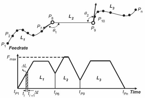
Figure 2.

CSBs with Cubic Bezier curves and a feedrate profile.

This figure describes how a linear segment set may be divided into several CSB areas and linear segment regions by break points $P_8$ and $P_9$. A corner error arising from system dynamics and geometry limits the corner feedrate. In comparison, the maximum feedrate for a cubic Bezier curve is calculated using the curvature, the permissible maximum machining speed, and the feedrate assigned. The trapezoidal feed rate profile is used to design feedrate acceleration and deceleration. The feed length per sample period, $∆L$, is calculated from the resultant feedrate profile, and the interpolated locations are calculated.

The first step in using the CSB criteria is determining the break points, or the critical corner angle. This study uses a first-order approximation of a feedforward servo system as the system model to complete interpolation and motion control in one sample time. As a result, the tracking error e may be stated as [24].

$$e=F\frac{1-k_f}{k_p}$$E12

as illustrated in Figure 3, where $F$ is the feedrate, $k_f$ is the feedforward gain, and $k_p$ is the position gain.

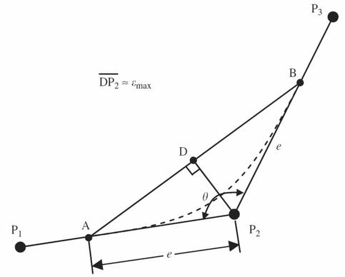
Figure 3.

An isosceles triangle approach is depicted schematically.

$\overline{P_1{P}_2}$ and $P_2{P}_3$ are two linked linear blocks with a corner angle y. On $P_1{P}_2$, its tracking error is e. Corner errors will occur when the cutting tool goes down the straight lines $\overline{P_1{P}_2}$ and $P_2{P}_3$, beginning at point $A$. The dashed line represents the actual tool path. Huang [24] presented an isosceles triangle approach to limit the maximum corner error ${\epsilon }_{\mathit{max}}$. When considering the geometrical connection of the isosceles triangle $∆A{P}_{2}B$, the height of the isosceles triangle $P_{2}D$ reflects the upper bound of the maximum corner error ${\epsilon }_{\mathit{max}}$, which is given by Eq. (13)

$$\frac{{\epsilon }_{\mathit{max}}}{e}=cos\frac{\theta }{2}$$E13

The connections between the prescribed feedrate $F_{\mathit{NC}}$, the maximum corner error ${\epsilon }_{\mathit{max}}$, and the critical corner angle ${\theta }_{\mathit{\text{critical}}}$ are derived by subtracting e from Eqs. (12) and (13).

$${\theta }_{\mathit{\text{critical}}}=2{cos}^{-1}\left(\frac{k_p}{1-k_f}\frac{{\epsilon }_{\mathit{max}}}{F_{\mathit{NC}}}\right)$$E14

The FBI’s interpolation technique is demonstrated using five CSBs. $\overline{P_0{P}_1}$ is the initial block in Figure 4, $\overline{P_1{P}_2}-\overline{P_3{P}_4}$ are the intermediate blocks, and $\overline{P_{41}{P}_5}$ is the last block. We’ll start with the center blocks. Because the interpolated block is $\overline{P_2{P}_3}$, the basis segment is made up of $\overline{P_1{P}_2},\overline{P_2{P}_3}$, and $\overline{P_3{P}_4}$, as seen in Figure 4b. As a result, the FBI may interpolate a Bezier curve $\overline{P_2{P}_3}$ using a control polygon $Q_0{Q}_1{Q}_2{Q}_3$ and parameters ($t_1$ and $t_2$). $\overline{P_1{P}_2}$, $\overline{P_2{P}_3}$, and $\overline{P_3{P}_4}$ are the three middle blocks that have distinct control polygons and may be interpolated into three separate Bezier curve segments, $\overline{P_1{P}_2}$, $\overline{P_2{P}_3}$, and $\overline{P_3{P}_4}$.

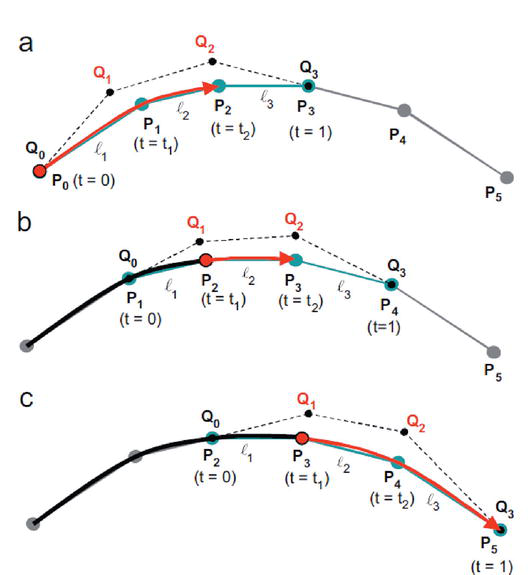
Figure 4.

The FBI interpolates five CSBs: (a) the first and second CSB blocks; (b) the third CSB block; and (c) the fourth and final CSB blocks.

4.2 Quintic triangular Bézier patch using dataset’s virtual mesh

Liu and Mann [25] introduced a piecewise interpolation polynomial by producing a quintic triangular Bézier patch for each data point using a Bézier control point based on the virtual mesh of the provided dataset. The resulting surface, however, only obtained $G^1$.

A triangular Bezier patch of degree n is given by

$$K\left(u,v,w\right)=\sum _{i+j+k=n}{P}_{i,j,k}{B}_{i,j,k}^n\left(u,v,w\right)$$E15

$$B_{i,j,k}^n\left(u,v,w\right)=\frac{n!}{i!j!k!}{u}^i{v}^j{w}^k$$E16

$\left(u,v,w\right)$ are barycentric coordinates, and the control points are $P_{i,j,k}$. Liu and Mann [25] constructed a piecewise triangular surface that interpolates data vertices onto a specified triangular mesh $M$. The number of incident edges for each data vertex $V$ is referred to as the valence of $V$. Because they assume M has arbitrary topology and is triangulated without singularities, $V^{\prime }s$ valence is always greater than 2. The mesh $M$ is likewise considered to be closed in their study.

Several conditions must be met in order for the triangular patches to connect with $G^1$ continuity, that is, for the tangent planes from the two adjoining patches to be coplanar at any point along the boundary curve. Figure 5 depicts two adjoining patches, $F_i$ and $F_{i-1}$, and their domain triangles for a vertex $V$ with a valence of $n$.

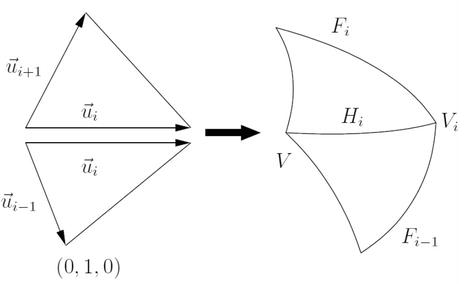
Figure 5.

Adjacent patches.

In domain triangles, the direction of the partial derivative along the $i$th edge of vertex $V$ is defined as ${\stackrel{⃑}{u}}_i$. $H_i\left(t\right)$ is the common boundary curve of patches $F_i$ and $F_{i-1}$, with $H_i\left(0\right)=V$and $H_i\left(1\right)=V_i$. If and only if there are scalar-valued functions $\beta \left(t\right),\rho \left(t\right),$and $\tau \left(t\right)$ such that

$${\beta }_i\left(t\right)\frac{\partial F_i}{\partial {\stackrel{⃑}{u}}_i}={\rho }_i\left(t\right)\frac{\partial F_i}{\partial {\stackrel{⃑}{u}}_{i+1}}+{\tau }_i\left(t\right)\frac{\partial F_{i-1}}{\partial {\stackrel{⃑}{u}}_{i-1}}.$$E17

$F_i$ and $F_{i-1}$ will join with $G^1$ continuity along $H_i\left(t\right)$.

To ensure that the tangents are properly oriented, we assume $\rho \left(t\right)\tau \left(t\right)\ge 0$.

Eq. (18) must hold for each pair of neighboring patches in order for patches to meet around vertex $V$ and connect with $G^1$ continuity. When Eq. (16) is differentiated in the direction of ui and evaluated at $t=0$, the following equation results:

$${\beta }_i^{\prime }\left(0\right)\frac{\partial F_i}{\partial {\stackrel{⃑}{u}}_i}+{\beta }_i\left(0\right)\frac{{\partial }^2{F}_i}{\partial {{\stackrel{⃑}{u}}_i}^2}={\beta }_i^{\prime }\left(0\right)\frac{\partial F_i}{\partial {\stackrel{⃑}{u}}_{i+1}}+{\beta }_i\left(0\right)\frac{{\partial }^2{F}_i}{\partial {\stackrel{⃑}{u}}_{i+1}\partial {\stackrel{⃑}{u}}_i}+v_i^{\prime }\left(0\right)\frac{\partial F_{i-1}}{\partial {\stackrel{⃑}{u}}_{i-1}}+v_i\left(0\right)\frac{{\partial }^2{F}_{i-1}}{\partial {\stackrel{⃑}{u}}_{i-1}\partial {\stackrel{⃑}{u}}_i}$$E18

By creating $n$ patches around vertex $V$, a set of equations from Eq. (20) must hold in order for $G^1$ continuity to exist along all borders; this is known as the twist compatibility or vertex consistency issue [26, 27]. In general, solving these equations necessitates solving circulant matrix problems [28]. Loop’s technique constructs boundary curves in such a way that the solutions to the twist terms are ensured [26]. The following are the steps of Loop’s sextic scheme:

1. Form quartic boundary polynomials.

2. Go through the twist phrases.

3. Create tangent fields around the edges.

4. Raise the border curve degree to sextic.

5. In the sextic patch, add the second row of control points to interpolate the tangent fields.

6. After averaging the control points from the previous stages, determine the remaining central control point (Figure 6).

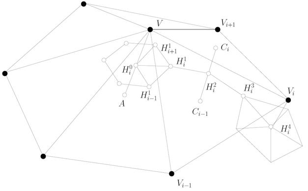
Figure 6.

Tangent boundary construction.

When the valences of the three vertices of a data triangle are identical, the patch formed by Loop’s method is quintic; if the three valences are all six, the patch degree decreases to quartic [26]. The boundary curves in Liu and Mann’s [25] method are constructed similarly to the first step of Loop’s scheme, but with the center control point set differently. The twist terms are solved in their scheme in the same way as Loop’s scheme is solved in the second stage. The first step will be reviewed briefly in this article; the specifics of the remaining parts of Loop’s system may be found in [26]. Loop produces the first two control points for each quartic boundary curve with control points of $H_i^0,\dots ,H_i^4$ as

$$H_i^0=\mathit{\mu V}+\left(1-\mu \right)A=\mathit{\mu V}+\frac{1-\mu }{n}\sum _{j=1}^n{V}_j$$E19

$$H_i^1=H_i^0+\frac{\mu }{n}\sum _{j=1}^n\left[cos\left(\frac{2\left(j-i\right)\pi }{n}\right)\right]V_j$$E20

Here, $n$ is the valence of the vertex $V$, and $A$ is the centroid of all of $V^{’}$s adjacent vertices. The generation of these control points involves performing a first-order Fourier transformation on all of $V^{’}$s surrounding vertices [28]. If all of the control points $H_i^0$ and $H_i^1$ are connected, they will create a normal $n-$gon with $V$ as the center, as illustrated in Figure 2. $\mu$ and $\eta$ are two shape parameters. When $\mu$ is equal to 1, the generated surface interpolates the data vertices. The tangent length at $V$ is defined by the parameter $\eta$. Loop proposes that $\mu$ and $\eta$ be used to create an appealing surface form.

$$\mu =\frac{1}{9}\left[4+cos\left(\frac{2\pi }{n}\right)\right],\eta =\frac{1}{3}\left[1+cos\left(\frac{2\pi }{n}\right)\right].$$E21

Eq. (22) calculates the final two control points $H_i^3$ and $H_i^4$ from the adjoining vertex $V_i$. The average of the two centroid points $C_i$ and $C_{i+1}$ of the two neighboring data triangles is used to get the middle point $H_i^2$:

$$H_i^2=\frac{C_{i-1}+C_i}{2}=\frac{V}{3}+\frac{V_i}{3}+\frac{V_{i+1}}{6}+\frac{V_{i-1}}{6}$$E22

4.3 Quadtree Bézier interpolation using uniformly distributed control points

Quadtree decomposition and Bézier interpolation have demonstrated a good ability to extract the image’s salient features in infrared and visual image fusion applications. Zhang et al. [29] have indeed developed an iterative quadtree decomposition and Bézier interpolation-based infrared and visual image fusion method. Each image patch is reconstructed using their approach by interpolating its four-by-four uniformly distributed control points, as seen below.

$$q_{i,j}\left(u,v\right)={\mathit{UMP}}_{i,j}{M}^T{V}^T,$$E23

where $\left(u,v\right)$ signifies the data point’s position and is represented by the ratio ranging from 0 to 1, $\left(U,V\right)$ symbolizes the position-related with coefficient, and $M$ represents the matrix of constant coefficients. $q_{i,j}$ represents the smoothed in image patch, and $P_{i,j}$ indicates the gray levels of $4\times 4$ uniformly distributed control points of $p_{i,j}$.

To be more specific

$$U=\left[{\upsilon }^3,{\upsilon }^2,{\upsilon }^1,{\upsilon }^0\right],V=\left[{\nu }^3,{\nu }^2,{\nu }^1,{\nu }^0\right],M=\left(\begin{array}{cc}\begin{array}{cc}-1& 3\\ 3& -6\end{array}& \begin{array}{cc}-3& 1\\ 3& 0\end{array}\\ \begin{array}{cc}-3& 3\\ 1& 0\end{array}& \begin{array}{cc}0& 0\\ 0& 0\end{array}\end{array}\right)$$E24

They used the Bézier interpolation approach to recreate each image patch twice in order to successfully extract the locally distributed bright and dark characteristics. That is, each image patch in the quadtree structure is built first by interpolating the local lowest gray values of the four-by-four uniformly distributed control points, and then a major portion of the bright features are eliminated from the reconstructed picture.

Second, each image patch in the quadtree structure is built further by interpolating the local maximum gray values of the four-by-four uniformly distributed control points; this allows the dark features to be eliminated from the reconstructed picture. As a result, the picture’s bright and dark characteristics may be successfully retrieved from the difference image of the original image and the smoothed image.

4.4 Tractable nonlinear interpolation framework using Bézier curves

Shimagaki and Barton [30] proposed a tractable nonlinear interpolation framework using Bézier curves. In addition to incorporating nonlinearity, this approach has the added advantage of conserving sums of categorical variables, which is not guaranteed under arbitrary nonlinear transformations of data. This property can be especially useful for conserved quantities such as probabilities. Historically, the Bézier method has been used in computer graphics to draw smooth curves.

Suppose a polynomial $p\left(t\right)$ that is sampled at discrete times $t_s$ for $s\in \left\{0,1,\dots ,K\right\}$. Thus, between two subsequent discrete time points $t_s$ and $t_{s+1}$, the interpolated value of the polynomial $p_B^{\left(s\right)}\left(t\right)$ is given by

$$p_B^{\left(s\right)}\left(t\right)=\sum _{n=0}^P{\beta }_n\left(\frac{t-t_s}{t_{s-1}-t_s}\right){\phi }_n^{\left(s\right)}\left(p{\left(t_{s^{\prime }}\right)}_{s^{\prime }=0}^K\right)$$E25

where ${\beta }_n$ is the nth Bernstein polynomial of degree $P$, with ${\beta }_n\left(\theta \right)=C_n^P{\theta }^n{\left(1-\theta \right)}^{P-n}\ge 0$. The control points ${\phi }_n^{\left(s\right)}\left(p{\left(t_{s^{\prime }}\right)}_{s^{\prime }=0}^K\right)$ is determined by the ensemble of data points $p{\left(t_{s^{\prime }}\right)}_{s^{\prime }=0}^K$ and defines the shape of the curve.

When choosing cubic (P = 3) interpolation for simplicity, but their technique may be extended to polynomials of varying degrees $P$. To ensure that the section at each interval $\left[t_s,t_{s+1}\right]$ for all $k$ is smoothly joined, we apply the following conditions:

$${\phi }_0^{\left(s\right)}\left({\left[p\left(t_{s^{\prime }}\right)\right]}_{s^{\prime }=0}^K\right)=p\left(t_s\right),$$E26

$${\phi }_3^{\left(s\right)}\left({\left[p\left(t_{s^{\prime }}\right)\right]}_{s^{\prime }=0}^K\right)=p\left(t_{s+1}\right).$$E27

The other control points ${\left\{{\phi }_1^{\left(s\right)},{\phi }_2^{\left(s\right)}\right\}}_{s=0}^{K-1}$ are reached by solving an optimization problem that represents the curves’ continuity and smoothness restrictions, For example, in Figure 7, cubic Bézier curves seamlessly interpolate between discretely sampled frequency trajectories generated by a Wright-Fisher model. Simulation parameters. $L=50$ sites, $N={10}^3$ population size, mutation rate $\mu ={10}^{-3}$, with simulations spanning $T=300$ generations. Data points are collected every $50$ generations and interpolated using cubic Bézier and linear interpolation.

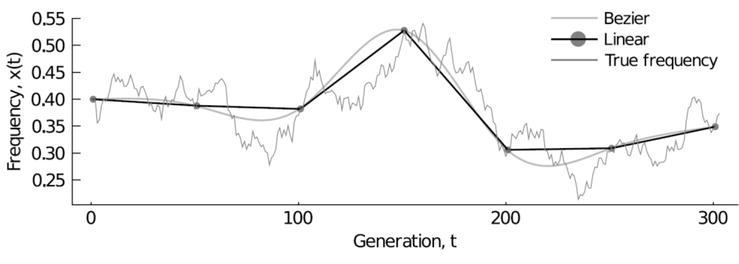
Figure 7.

Smooth curves are generated using Bézier interpolation.

5. Conclusions

In this chapter, unique and inventive methods for maximizing the benefits of various parametric polynomials are discussed. The four new recent polynomials are validated using various interpolation methods. As compared to existing methodologies and conventional procedures, the simulation properties clearly suggest that the examined polynomials may improve the quality of many applications. Additionally, the reviewed method may be used for a variety of image interpolation applications, including image zooming and rotation.

References

- 1.
Adcock RJ. Note on the method of least squares. The Analyst, Des Moines, Iowa. 1877; 4 :183-184 - 2.
ISO 10360-6. Geometrical Product Specifications (GPS)—Acceptance and Reverification Test for Coordinate Measuring Machines (CMM)—Part 6: Estimation of Errors in Computing Gaussian Associated Features. Geneva, Switzerland: ISO; 2001 - 3.
Pearson K. On lines and planes of closest fit to systems of points in space. The Philisophy Magazine. 1991; 2 (11):559-572 - 4.
Ahn SJ, Rauh W, Cho HS, Warnecke H-J. Orthogonal distance fitting of implicit curves and surfaces. IEEE Transactions on Pattern Analytical Machine Intellectual. 2002; 24 (5):620-638 - 5.
Ahn SJ, Westkämper E, Rauh W. Orthogonal distance fitting of parametric curves and surfaces. In: Levesley J et al., editors. Proc. 4th Int'l Symp. Algorithms for Approximation. UK: Univ. of Huddersfield; 2002. pp. 122-129 - 6.
Boggs PT, Byrd RH, Schnabel RB. A stable and efficient algorithm for nonlinear orthogonal distance regression. SIAM Journal of Science Statistical Computing. 1987; 8 :1052-1078 - 7.
Boggs PT, Donaldson JR, Byrd RH, Schnabel RB. Algorithm 676 – ODRPACK: Software for weighted orthogonal distance regression. ACM Transactions on Mathematical Software. 1989; 15 (4):348-364 - 8.
Cao X, Shrikhande N, Hu G. Approximate orthogonal distance regression method for fitting quadric surfaces to range data. Pattern Recognition Letters. 1994; 15 (8):781-796 - 9.
Helfrich H-P, Zwick D. A trust region method for implicit orthogonal distance regression. Numerical Algorithms. 1993; 5 :535-545 - 10.
Helfrich H-P, Zwick D. A trust region algorithm for parametric curve and surface fitting. Journal of Computational and Applied Mathematics. 1996; 73 :119-134 - 11.
Sullivan S, Sandford L, Ponce J. Using geometric distance fits for 3-D object Modeling and recognition. IEEE Transactions on Pattern Analytical Machine. Intellectual. 1994; 16 (12):1183-1196 - 12.
Butler BP, Forbes AB, Harris PM. Algorithms for Geometric Tolerance Assessment. NPL: Teddington, U.K; 1994 - 13.
Sourlier D. Three Dimensional Feature Independent Bestfit in Coordinate Metrology. Zurich, Switzerland: ETH Zurich; 1995 - 14.
Bookstein FL. Fitting conic sections to scattered data. Computer Graphical Image Processing. 1979; 9 (1):56-71 - 15.
Fitzgibbon A, Pilu M, Fisher RB. Direct Least Square fitting of ellipses. IEEE Transactions on Pattern Analytical Machine Intellectual. 1999; 21 (5):476-480 - 16.
Marshall D, Lukacs G, Martin R. Robust segmentation of primitives from range data in the presence of geometric degeneracy. IEEE Transactions on Pattern Analytical Machine Intellectual. 2001; 23 (3):304-314 - 17.
Solina F, Bajcsy R. Recovery of parametric models from range images: The case for Superquadrics with global deformations. IEEE Transactions on Pattern Analytical Machine Intellectual. 1990; 12 (2):131-147 - 18.
Taubin G. Estimation of planar curves, surfaces, nonplanar space curves defined by implicit equations with applications to edge and range image segmentation. IEEE Transactions on Pattern Analytical Machine Intellectual. 1991; 13 (11):1115-1138 - 19.
Ameer M, Abbas M, Abdeljawad T, Nazir T. A novel generalization of Bézier-like curves and surfaces with shape parameters. Mathematics. 2022; 10 (3):376 - 20.
Khan A, Iliyas M, Khan K, Mursaleen M. Approximation of conic sections by weighted Lupaş post-quantum Bézier curves. Demonstratio Mathematica. 2022; 55 (1):328-342 - 21.
Özger F. On new Bézier bases with Schurer polynomials and corresponding results in approximation theory. Communications Faculty of Sciences University of Ankara Series A1 Mathematics and Statistics. 2020; 69 (1):376-393 - 22.
Lepot M, Aubin JB, Clemens F. Interpolation in time series: An introductive overview of existing methods, their performance criteria and uncertainty assessment. Water. 2017; 9 (10):796 - 23.
Yau H-T, Wang J-B. Fast Bezier interpolator with real-time Lookahead function for high-accuracy machining. International Journal of Machine Tools and Manufacture. 2007; 47 (10):1518-1529 - 24.
Huang YS. The Research on Acceleration/Deceleration Algorithms for CNC Motion Control. Taiwan: Department of Mechanical Engineering, National Chung Cheng University; 1996 - 25.
Liu Y, Mann S. Parametric triangular Bézier surface interpolation with approximate continuity. In: Proceedings of the 2008 ACM Symposium on Solid and Physical Modeling. New York, NY: ACM Press; 2008. pp. 381-387 - 26.
Loop C. A G1 triangular spline surface of arbitrary topological type. Computer Aided Geometric Design. 1994; 11 - 27.
Van Wijk J. Bicubic patches for approximating nonrectangular control-point meshes. Computer Aided Geometric Design. 1986; 3 - 28.
Davis P. Circulant Matrices. New York: Wiley; 1979 - 29.
Zhang Y, Zhang L, Shen J, Zhang S, Bai X. Infrared and visual image fusion via iterative quadtree decomposition and Bézier interpolation. In: Fourteenth International Conference on Digital Image Processing (ICDIP 2022). Vol. 12342. Wuhan, China: SPIE; 2022. pp. 730-738 - 30.
Shimagaki K, Barton JP. Bézier interpolation improves the inference of dynamical models from data. Physical Review E. 2023; 107 (2):024116