Perspective Chapter: On Entanglement Measures – Discrete Phase Space and Inverter-Chain Link Viewpoint

Abstract

In contrast to abstract statistical analyses in the literature, we present a concrete physical diagrammatic model of entanglement characterization and measure with its underlying discrete phase-space physics. This paper serves as a pedagogical treatment of this complex subject of entanglement measures. We review the important inherent concurrence property of entangled qubits, as well as underscore its emergent qubit behavior. From the discrete phase space point of view, concurrence translates to translation symmetry of entangled binary systems in some quantitative measure of entanglement. Although the focus is on bipartite system, the technique is readily extendable to multi-partite system of qubits, as can easily be deduced from the physical inverter-chain link model. A diagrammatic analysis of the entanglement of formation for any multi-partite qubit system is given. We show that quantum mechanical joint distribution are entanglements.

1. Introduction

Quantum entanglement has developed from a mere intellectual curiosity [1] of the fundamental structure of quantum mechanics¹ to become an important and practical resource for quantum information processing in the evolving theory of quantum information and ultra-fast computing. Thus, the quantitative measure of entanglement has developed into one of the most active fields of theoretical and experimental research. Here we will try to shed more light on some of the important concepts in the quantification of quantum entanglement by using a concrete simple mechanical model of a bipartite system of qubits or chain of qubits. This treatment will be in contrast with mostly abstract and statistical treatment of entanglement measure in the literature.

We will focus on the so-called entanglement of formation and concurrence, two of the most important concepts to characterize entanglement resource. Here we consider a qubit as a two-state system. Moreover, we also consider an entangled qubit as effectively a two-state system, an emergent qubit as depicted in our physical inverter-chain link model. A two-state system has a unity entropy. Thus, a maximally entangled state has entropy equal to 1. From the discrete phase space point of view, any two-state system can be considered to possess two lattice-site states. Discrete Fourier transform or Hadamard transform implements unitary superposition of the two lattice-site states (also referred to as ‘Wannier functions’) to yield a sort of crystal-momentum states (also referred to as ‘Bloch functions’). For example, take the $\left|00\right.⟩$ and $\left|11\right.⟩$ ‘lattice-site states’, then the Hadamard bijective discrete transformation gives the’crystal-momentum states’, ${\mathrm{\Phi }}^{+}$ and ${\mathrm{\Phi }}^{-}$, which are two of the Bell basis states (or’Bloch function’ states).

2. Bell basis deduced from inverter-chain link model

We sketch here the derivation of the Bell basis states from our physical model, as depicted in Figure 1. Clearly, the entanglement of two bare qubits is divided into two orthogonal spaces of triplet² and singlet entanglement states.

Figure 1.

Physical diagrammatic model of “triplet” (left) and singlet (right) entanglement. By construction, each diagram is viewed as a two-state system, respectively. The Bell basis are readily derived below each diagram, using the Hadamard transformation. The actual physical implementation of the chain of inverters may need frictionless male/female sliding tube coupling for large-angle swing, but this is beside the point. We assume a rigid coupling model for simultaneity of events at both ends.

Since the Hadamard transform is unitary, the inverse transform is well-defined, i.e., the transformation is bijective. We refer to $\left\{\left|00\right.⟩,\left|11\right.⟩\right\}$ as the “Wannier functions” space and the $\left\{\left|{\mathrm{\Phi }}^{+}\right.⟩,\left|{\mathrm{\Phi }}^{-}\right.⟩\right\}$ as the corresponding “Bloch functions” space of a two-state triplet entanglement system. Likewise, $\left\{\left|01\right.⟩,\left|10\right.⟩\right\}$ as the “Wannier functions” space and the $\left\{\left|{\mathrm{\Psi }}^{+}\right.⟩,\left|{\mathrm{\Psi }}^{-}\right.⟩\right\}$ as the corresponding “Bloch functions” space of a two-state singlet entanglement system.

By virtue of this bijective relationship, any function of Wannier functions will have a corresponding function of Bloch functions. For example, a maximally mixed Wannier function states will generate a maximally mixed Bloch function states or the so-called maximally mixed entanglement states. Mixed and pure states will be further discussed below.

3. Entangled qubits as an emergent qubit

The virtue of our inverter-chain link model is that the emergent two-state property of entangled qubits is very transparent, since changing the state of one of the qubits also immediately change the states of the rest of the entangled partner(s)³. Here, we will rigorously justify our claim that entangled qubits behave, as a whole, as an emergent qubit.

Here, we employ the matrix representation of states and operators. We now represent $\left|{\mathrm{\Phi }}^{+}\right.⟩$ and$\left|{\mathrm{\Phi }}^{-}\right.⟩$ as,

$$\left|{\mathrm{\Phi }}^{+}\right.⟩=\frac{1}{\sqrt{2}}\left(\begin{array}{c}1\\ 1\end{array}\right),$$E1

$$\left|{\mathrm{\Phi }}^{-}\right.⟩=\frac{1}{\sqrt{2}}\left(\begin{array}{c}1\\ -1\end{array}\right).$$E2

Then we have

$$\left.⟨{\mathrm{\Phi }}^{+}\right|{\sigma }_x\left|{\mathrm{\Phi }}^{+}\right.⟩=\frac{1}{2}\left(11\right)\left(\begin{array}{cc}0& 1\\ 1& 0\end{array}\right)\left(\begin{array}{c}1\\ 1\end{array}\right)=1,$$E3

$$\left.⟨{\mathrm{\Phi }}^{-}\right|{\sigma }_x\left|{\mathrm{\Phi }}^{-}\right.⟩=\frac{1}{2}\left(\begin{array}{cc}1& -1\end{array}\right)\left(\begin{array}{cc}0& 1\\ 1& 0\end{array}\right)\left(\begin{array}{c}1\\ -1\end{array}\right)=-1,$$E4

proving the two eigenvalues, like a qubit property of the triplet system.

For the singlet the most straightforward manipulation is to recognize that the singlet system is an independent system with its own two states which is orthogonal to the triplet states. In this sense we can also represent the singlet states just like that of the triplet states, namely,

$$\left|{\mathrm{\Psi }}^{+}\right.⟩=\frac{1}{\sqrt{2}}\left(\begin{array}{c}1\\ 1\end{array}\right),$$E5

$$\left|{\mathrm{\Psi }}^{-}\right.⟩=\frac{1}{\sqrt{2}}\left(\begin{array}{c}1\\ -1\end{array}\right).$$E6

Note that in the ‘Bloch-state” space, ${\sigma }_z$ in the “Wannier-state” space is transform to ${\sigma }_x$ in entangled states,

$${\sigma }_x=H{\sigma }_{z}H=\left(\begin{array}{cc}0& 1\\ 1& 0\end{array}\right).$$E7

Thus, we also have for the singlet states

$$\left.⟨{\mathrm{\Psi }}^{+}\right|{\sigma }_x\left|{\mathrm{\Psi }}^{+}\right.⟩=\frac{1}{2}\left(\begin{array}{cc}1& 1\end{array}\right)\left(\begin{array}{cc}0& 1\\ 1& 0\end{array}\right)\left(\begin{array}{c}1\\ 1\end{array}\right)=1,$$E8

$$\left.⟨{\mathrm{\Psi }}^{-}\right|{\sigma }_x\left|{\mathrm{\Psi }}^{-}\right.⟩=\frac{1}{2}\left(\begin{array}{cc}1& -1\end{array}\right)\left(\begin{array}{cc}0& 1\\ 1& 0\end{array}\right)\left(\begin{array}{c}1\\ -1\end{array}\right)=-1.$$E9

Following this notion, Eqs. (8) and (9) can easily be extended to all entangled qubits, bipartite or multi-partite qubit systems to yield an emergent qubit. It is far more simpler to analyze the inverter-chain link diagrams, i.e., employ diagrammatic analyses.

4. Translational/shift invariance of Bell basis

The translational invariance of maximally entangled Bell basis states demonstrates a unique characteristic of entangled qubits. This unique property has been used to detect or measure how much entanglement is present in arbitrary pure and mixed states. This is implemented in terms of the notion of concurrence, to be elaborated below.

The translational or shift operation (also referred to as the flip operation in the literature) is demonstrated here for the Bell Basis states and their superpositions. First, let us consider all the Bell basis states. We have,

$${\mathrm{\Phi }}^{+}=\frac{1}{\sqrt{2}}\left(\left|0\right.⟩\left|0\right.⟩+\left|1\right.⟩\left|1\right.⟩\right).$$E10

Upon applying the translation (shift by $+1\left(\mathit{mod}2\right)$) operator, $T\left(+1\right)$, we obtain

$$\begin{array}{lll}T\left(+1\right){\mathrm{\Phi }}^{+}& =& \frac{1}{\sqrt{2}}\left(\left|0+1\right.⟩\left|0+1\right.⟩+\left|1+1\right.⟩\left|1+1\right.⟩\right),\\ & =& \frac{1}{\sqrt{2}}\left(\left|1\right.⟩\left|1\right.⟩+\left|0\right.⟩\left|0\right.⟩\right)={\mathrm{\Phi }}^{+},\end{array}$$E11

where addition obeys modular arithmetic (mod 2). The ‘plus’ entangled basis states are even upon the operation of T(+1), whereas the ‘minus’ entangled basis states are odd when operated by T(+1). We still consider the shited, $-{\mathrm{\Phi }}^{-}$ and $-{\mathrm{\Psi }}^{-},$as invariant since it differs from the unshifted Bell states by a global phase factor. In the literature this translation operation is the so-called flipping operation first used by Wooters, et al., [2, 3].

4.1 Translational property of maximal superposition of Bell basis

Now let us consider the superposition of maximally entangled Bell basis states. We can easily see that a superposition of ‘plus’ entangled basis states with ‘minus’ entangled basis states yield unentangled basis states. For example, we have,

$$\begin{array}{l}\frac{1}{\sqrt{2}}\left({\mathrm{\Phi }}^{+}+{\mathrm{\Phi }}^{-}\right)=\left|0\right.⟩\left|0\right.⟩,\end{array}$$E12

$$\begin{array}{c}\frac{1}{\sqrt{2}}\left({\mathrm{\Phi }}^{+}-{\mathrm{\Phi }}^{-}\right)=\left|1\right.⟩\left|1\right.⟩.\end{array}$$E13

The thing to notice is that although the superposition is made up of two maximally entangled Bell basis, the results are not shift invariant (i.e., generation of another Wannier state yields Wannier state located at another site, which is orthogonal to the unshifted one). This means that the superposition given above yields unentangled states (product states) in Eq. (13). In what follows, we will see that only the following combination of entangled basis states yields another entangled basis states as long as they both belong to either ‘even’ or ‘odd’ spaces. We have, by diagrammatic construction,

$${\mathit{\text{triplet}}}^{\pm }\otimes {\mathit{\text{triplet}}}^{\pm }={\mathit{\text{triplet}}}^{\pm }\text{or}{\mathit{\text{singlet}}}^{\pm },$$E14

$${\mathit{\text{triplet}}}^{\pm }\otimes {\mathit{\text{singlet}}}^{\pm }={\mathit{\text{singlet}}}^{\pm }\text{or}{\mathit{\text{triplet}}}^{\pm },$$E15

$${\mathit{\text{singlet}}}^{\pm }\otimes {\mathit{\text{singlet}}}^{\pm }={\mathit{\text{triplet}}}^{\pm }\text{or}{\mathit{\text{singlet}}}^{\pm }.$$E16

Equation (15) is quite interesting because it holds on a complete expansion of a direct product of two qubit states. These relations can easily be deduced from the physical diagrammatic model, see Figure 1. For example, if we define the operation as a superposition such as,

$$\frac{1}{\sqrt{2}}\left({\mathrm{\Phi }}^{+}+{\mathrm{\Psi }}^{+}\right)=\left[\frac{1}{\sqrt{2}}\left(\left|1\right.⟩+\left|0\right.⟩\right)\otimes \frac{1}{\sqrt{2}}\left(\left|1\right.⟩+\left|0\right.⟩\right)\right].$$E17

We see that Eq. (17) is a direct product state of two qubits. We will see in what follows that this is an entangled state and corresponds to Eq. (15) of the ${\mathit{\text{singlet}}}^{+}$ or ${\mathit{\text{triplet}}}^{+}$ of the model diagrams depending on the actual linkage. Similarly, we have,

$$\frac{1}{\sqrt{2}}\left({\mathrm{\Phi }}^{-}+{\mathrm{\Psi }}^{-}\right)=\left[\frac{1}{\sqrt{2}}\left(\left|1\right.⟩+\left|0\right.⟩\right)\otimes \frac{1}{\sqrt{2}}\left(\left|1\right.⟩-\left|0\right.⟩\right)\right],$$E18

corresponds to Eq. (15) of the $\mathit{\text{singlet}}$ or $\mathit{\text{triplet}}$ of the model diagrams, depending on the actual linking.

However, the following combinations of ‘even’ and ‘odd’ entangled states result in unentangled states, namely,

$$\frac{1}{\sqrt{2}}\left({\mathrm{\Phi }}^{+}+{\mathrm{\Psi }}^{-}\right)=\frac{1}{2}\left[\left(\left|1\right.⟩\left|1\right.⟩+\left|0\right.⟩\left|0\right.⟩\right)+\left(\left|0\right.⟩\left|1\right.⟩-\left|1\right.⟩\left|0\right.⟩\right)\right],$$E19

and

$$\frac{1}{\sqrt{2}}\left({\mathrm{\Phi }}^{-}+{\mathrm{\Psi }}^{+}\right)=\frac{1}{2}\left[\left(\left|1\right.⟩\left|1\right.⟩-\left|0\right.⟩\left|0\right.⟩\right)+\left(\left|0\right.⟩\left|1\right.⟩+\left|1\right.⟩\left|0\right.⟩\right)\right],$$E20

by virtue of the failure to have global sign factors. All these claims are justified through the concept of concurrence, an inherent property of entangled qubits, to be discussed in what follows. Moreover, this feature of failing to have global sign factor is also reflected in the failure to represent by our inverter-chain link diagrams.

5. Bipartite system

Let the Hilbert spaces of a bipartite system consisting of A and B be denoted by ${\mathrm{\mathscr{H}}}_A$ and ${\mathrm{\mathscr{H}}}_B$, respectively. A bipartite system is a system with Hilbert space equal to the direct product of ${\mathrm{\mathscr{H}}}_A$ and ${\mathrm{\mathscr{H}}}_B$, i.e.,

$${\mathrm{\mathscr{H}}}_{\mathit{AB}}={\mathrm{\mathscr{H}}}_A\otimes {\mathrm{\mathscr{H}}}_B$$E21

Let the density matrix for the whole system be denoted by $\rho$. Then the reduced density matrix of a subsystem $A$ is given by the partial trace,

$${\rho }_A={\mathit{Tr}}_B\rho .$$E22

The entanglement entropy, $S_A$, is the von Newmann entropy of the reduced density matrix, ${\rho }_A$,

$$S_A=-\mathit{Tr}{\rho }_{A}log{\rho }_A.$$E23

Example 1 Let $\mathrm{\Omega }$ be the number of distinct states in subsystem A_. assume a uniform distribution among states, hence ${\rho }_A$ has eigenvalues $\frac{1}{\mathrm{\Omega }}$, i.e., ${\rho }_A$ can be represented by a diagonal $\mathrm{\Omega }\times \mathrm{\Omega }$ matrix with identical matrix elements given by $\frac{1}{\mathrm{\Omega }}$. Thus, in taking the trace we can use the eigenvalues of the reduced density matrix operator, ${\rho }_A$. Therefore, we have

$$\begin{array}{lll}{S}_A& =& -\mathit{Tr}\frac{1}{\mathrm{\Omega }}log\frac{1}{\mathrm{\Omega }},\\ & =& log\mathrm{\Omega }.\end{array}$$E24

Upon multiplying by the Boltzmann constant, $k_B$, we obtain

$$k_B{S}_A=k_{B}log\mathrm{\Omega },$$E25

which is the Boltzmann thermodynamic entropy, based on ergodic theorem.

Example 2. Two qubit system.

A qubit is simply a quantum bit whose number of distinct eigenstates is 2. We denote these eigenstates as $\left|0\right.⟩$ and $\left|1\right.⟩$, i.e., a two-state system. If each subsystem A or B is a single qubit, then the Hilbert space of the whole system is span by the following 4 direct product states, namely,

$$\left|00\right.⟩,\left|01\right.⟩,\left|10\right.⟩,\left|11\right.⟩.$$E26

Here, the first bit refers to subsystem A and the second bit refers to subsystem B. Now, the density matrix of a pure state is,

$$\rho =\left|\psi \right.⟩\left.⟨\psi \right|,$$E27

then

$$\begin{array}{lll}{\rho }^2& =& \left|\psi \right.⟩\left|\psi \right.⟩\left.⟨\psi \right|\left|\psi \right.⟩\left.⟨\psi \right|,\\ & =& \rho .\end{array}$$E28

An operator whose square is equal to itself must have an eigenvalue equal to unity. Let us write for pure state of the two qubits as,

$$\left|\psi \right.⟩=\frac{1}{\sqrt{2}}\left(\left|00\right.⟩+\left|11\right.⟩\right),$$E29

$$\left.⟨\psi \right|=\frac{1}{\sqrt{2}}\left(\left.⟨00\right|+\left.⟨11\right|\right).$$E30

We have,

$$\left.⟨\psi \right|\left|\psi \right.⟩=1.$$E31

Thus, indeed,

$$\begin{array}{lll}{\rho }^2& =& \left|\psi \right.⟩\left.⟨\psi \right|\left|\psi \right.⟩\left.⟨\psi \right|,\\ & =& \left|\psi \right.⟩\left.⟨\psi \right|=\rho .\end{array}$$E32

We refer to $\left|\psi \right.⟩$ as a maximally entangled state in the sense that the first qubit is exactly “link” to the second qubit. The reduced density matrix for subsystem A is

$${\rho }_A={\mathit{Tr}}_B\rho =\frac{1}{2}\left(\left|0_A\right.⟩\left.⟨0_A\right|+\left|1_A\right.⟩\left.⟨1_A\right|\right).$$E33

Now clearly

$$\begin{array}{lll}{\rho }_A^2& =& \frac{1}{4}\left(\left|0_A\right.⟩\left.⟨0_A\right|+\left|1_A\right.⟩\left.⟨1_A\right|\right)\left(\left|0_A\right.⟩\left.⟨0_A\right|+\left|1_A\right.⟩\left.⟨1_A\right|\right),\\ & =& \frac{1}{4}\left(\left|0_A\right.⟩\left.⟨0_A\right|+\left|1_A\right.⟩\left.⟨1_A\right|\right)=\frac{1}{2}{\rho }_A,\end{array}$$E34

so that ${\rho }_A$ is not a pure state but mixed, i.e., a mixture of two pure states, $\left|0_A\right.⟩$ and $\left|1_A\right.⟩$. Note that the mixed states density matrix do not possess off-diagonal elements. From the last identity, the eigenvalues of ${\rho }_A$ is $\frac{1}{2}$ and since the subsystem A is a single qubit with two distinct states, then eigenvalues of ${\rho }_A$ corresponds to $\frac{1}{\mathrm{\Omega }}$ of our first example above. Thus we refer to ${\rho }_A$ as “uniformly’” mixed often referred to as “maximally mixed” with the initial state $\left|\psi \right.⟩$ as “maximally entangled”.

6. Entanglement of formation of multi-partite qubit systems

The entanglement entropy of subsystem A can be calculated using the eigenvalues of the 2 × 2 matrix of ${\rho }_A$, which is ${\lambda }_A=\frac{1}{2}$. Therefore, we have for the entanglement entropy or entanglement of formation given by,

$$\begin{array}{lll}{S}_A& =& -\mathit{Tr}{\rho }_{A}log{\rho }_A,\\ & =& -\mathit{Tr}\frac{1}{2}log\frac{1}{2}=log{2}^1,\end{array}$$E35

where exponent base 2, here 1, is the number of qubits that is entangled with system B. This will be made clear in the next example.

Example 3 A four qubit system:

If each subsystem A or B has two qubits, then the Hilbert space of the whole system is span by the following 16 direct product states, i.e., $2^4=16$ states. The maximally entangled pure state is determined by the following eight diagrams [4], see Figure 2, and their flipped or translated states,

Figure 2.

Two-state eight diagrams for entangled four qubits. The so-called flip operation yields the second state for each of the above diagrams. The entangled basis is constructed by the superposition, via the Hadamard transformation, of each diagram and its corresponding flipped diagram. [Reproduced from Ref. [4]].

Any combination or superposition of both ‘even’ triplet and singlet states comprised a maximally entangled state, i.e.,

$$\left(\begin{array}{c}{\mathrm{\Phi }}_1^{+}\\ {\mathrm{\Phi }}_1^{-}\end{array}\right)=\frac{1}{\sqrt{2}}\left(\begin{array}{cc}1& 1\\ 1& -1\end{array}\right)\left(\begin{array}{c}\left|0\right.⟩\left|0\right.⟩\left|0\right.⟩\left|0\right.⟩\\ \left|1\right.⟩\left|1\right.⟩\left|1\right.⟩\left|1\right.⟩\end{array}\right),$$E36

$$\left(\begin{array}{c}{\mathrm{\Phi }}_8^{+}\\ {\mathrm{\Phi }}_8^{-}\end{array}\right)=\frac{1}{\sqrt{2}}\left(\begin{array}{cc}1& 1\\ 1& -1\end{array}\right)\left(\begin{array}{c}\left|0\right.⟩\left|1\right.⟩\left|0\right.⟩\left|1\right.⟩\\ \left|1\right.⟩\left|0\right.⟩\left|1\right.⟩\left|0\right.⟩\end{array}\right).$$E37

Thus, from the states given above, we have for example the maximally entangled state,

$$\left|\psi \right.⟩=\frac{1}{\sqrt{2}}\left({\mathrm{\Phi }}_1^{+}+{\mathrm{\Phi }}_8^{+}\right),$$E38

and similarly, we can also form another entangled state,

$$\left|\psi \right.⟩=\frac{1}{\sqrt{2}}\left({\mathrm{\Phi }}_1^{-}+{\mathrm{\Phi }}_8^{-}\right),$$E39

where the first two bits belongs to subsystem A and the second two bits belong to subsystem B. We note that

$$\left.⟨\psi \right|\left|\psi \right.⟩=1.$$E40

Therefore

$$\begin{array}{lll}{\rho }^2& =& {\left(\left|\psi \right.⟩\left.⟨\psi \right|\right)}^2,\\ & =& \left|\psi \right.⟩\left.⟨\psi \right|=\rho .\end{array}$$E41

So $\left|\psi \right.⟩$ is a pure state.

In general, the following maximally entangled state corresponds to a chain of entangled basis states, namely,

$$\left|{\psi }^{+}\right.⟩=\frac{1}{\sqrt{8}}\left({\mathrm{\Phi }}_1^{+}+{\mathrm{\Phi }}_2^{+}+{\mathrm{\Phi }}_3^{+}+{\mathrm{\Phi }}_4^{+}+{\mathrm{\Phi }}_5^{+}+{\mathrm{\Phi }}_6^{+}+{\mathrm{\Phi }}_7^{+}+{\mathrm{\Phi }}_8^{+}\right),$$E42

$$\left|{\psi }^{-}\right.⟩=\frac{1}{\sqrt{8}}\left({\mathrm{\Phi }}_1^{-}+{\mathrm{\Phi }}_2^{-}+{\mathrm{\Phi }}_3^{-}+{\mathrm{\Phi }}_4^{-}+{\mathrm{\Phi }}_5^{-}+{\mathrm{\Phi }}_6^{-}+{\mathrm{\Phi }}_7^{-}+{\mathrm{\Phi }}_8^{-}\right),$$E43

of a four qubit system.

The density matrix operator for the whole 4-qubit system can be written as,

$$\rho =\frac{1}{\sqrt{2}}\left(\left|{\mathrm{\Phi }}_1^{-}+{\mathrm{\Phi }}_8^{-}\right.⟩\right)\frac{1}{\sqrt{2}}\left(\left.⟨{\mathrm{\Phi }}_1^{-}+{\mathrm{\Phi }}_8^{-}\right|\right),$$E44

$$\rho =\frac{1}{4}\left[\left|00,00\right.⟩+\left|01,01\right.⟩+\left|10,10\right.⟩+\left|11,11\right.⟩\right]\left[\left.⟨00,00\right|+\left.⟨01,01\right|+\left.⟨10,10\right|+\left.⟨11,11\right|\right].$$E45

The reduced density matrix operator for subsystem A is again obtained by taking partial trace with respect to subsystem B.

$$\begin{array}{lll}{\rho }_A& =& {\mathit{Tr}}_B\rho ,\\ & =& \left.⟨{00}_B\right|\rho \left|{00}_B\right.⟩+\left.⟨{01}_B\right|\rho \left|{01}_B\right.⟩+\left.⟨{10}_B\right|\rho \left|{10}_B\right.⟩+\left.⟨{11}_B\right|\rho \left|{11}_B\right.⟩,\\ & =& \frac{1}{4}\left|{00}_A\right.⟩\left.⟨{00}_A\right|+\left|{01}_A\right.⟩\left.⟨{01}_A\right|+\left|{10}_A\right.⟩\left.⟨{10}_A\right|+\left|{11}_A\right.⟩\left.⟨{11}_A\right|.\end{array}$$E46

To determine the eigenvalues for ${\rho }_A$, we take its square,

$$\begin{array}{lll}{\rho }_A^2& =& \frac{1}{16}\left(\left|{00}_A\right.⟩\left.⟨{00}_A\right|+\left|{01}_A\right.⟩\left.⟨{01}_A\right|+\left|{10}_A\right.⟩\left.⟨{10}_A\right|+\left|{11}_A\right.⟩\left.⟨{11}_A\right|\right),\\ & & \times \left(\left|{00}_A\right.⟩\left.⟨{00}_A\right|+\left|{01}_A\right.⟩\left.⟨{01}_A\right|+\left|{10}_A\right.⟩\left.⟨{10}_A\right|+\left|{11}_A\right.⟩\left.⟨{11}_A\right|\right),\\ & =& \frac{1}{16}\left(\left|{00}_A\right.⟩\left.⟨{00}_A\right|+\left|{01}_A\right.⟩\left.⟨{01}_A\right|+\left|{10}_A\right.⟩\left.⟨{10}_A\right|+\left|{11}_A\right.⟩\left.⟨{11}_A\right|\right),\\ & =& \frac{1}{4}{\rho }_A.\end{array}$$E47

So we have

$${\rho }_A^2=\frac{1}{4}{\rho }_A$$E48

and the eigenvalues of ${\rho }_A$ is $\frac{1}{4}$. We can now calculate the entanglement entropy of subsystem A. We have

$$\begin{array}{lll}{S}_A& =& -\mathit{Tr}{\rho }_{A}log{\rho }_A,\\ & =& log{2}^2.\end{array}$$E49

The exponent 2 correspond to the number of qubits that is entangled with subsystem B. In general, for maximally entangled bipartite system A and B, each having k number of qubits $S_A$ is given by,

$$S_A=log{2}^k.$$E50

Now of course, for this bipartite system,

$$S_A=S_B,$$E51

which simply means a complete matching of configurations of each system A and B, respectively, otherwise some degrees of freedom will be hanging, not matched or cannot be entangled.

Example 4. Tripartite system of three qubits:

The following diagrams represent the entangled tripartite system of qubits (Figure 3).

Figure 3.

Two-state four diagrams for entangled three qubits of a tripartite system. Flip operations yield the respective second states. [Reproduced from Ref. [4]].

The entangled basis states are as follows,

$$\left(\begin{array}{c}{\mathrm{\Xi }}^{+}\\ {\mathrm{\Xi }}^{-}\end{array}\right)=\frac{1}{\sqrt{2}}\left(\begin{array}{cc}1& 1\\ 1& -1\end{array}\right)\left(\begin{array}{c}\left|0\right.⟩\left|1\right.⟩\left|1\right.⟩\\ \left|1\right.⟩\left|0\right.⟩\left|0\right.⟩\end{array}\right),$$E52

$$\left(\begin{array}{c}{\mathrm{\Theta }}_3^{+}\\ {\mathrm{\Theta }}_3^{--}\end{array}\right)=\frac{1}{\sqrt{2}}\left(\begin{array}{cc}1& 1\\ 1& -1\end{array}\right)\left(\begin{array}{c}\left|0\right.⟩\left|0\right.⟩\left|0\right.⟩\\ \left|1\right.⟩\left|1\right.⟩\left|1\right.⟩\end{array}\right),$$E53

$$\left(\begin{array}{c}{\mathrm{\Omega }}^{+}\\ {\mathrm{\Omega }}^{-}\end{array}\right)=\frac{1}{\sqrt{2}}\left(\begin{array}{cc}1& 1\\ 1& -1\end{array}\right)\left(\begin{array}{c}\left|0\right.⟩\left|1\right.⟩\left|0\right.⟩\\ \left|1\right.⟩\left|0\right.⟩\left|1\right.⟩\end{array}\right),$$E54

$$\left(\begin{array}{c}{\mathrm{\Gamma }}^{+}\\ {\mathrm{\Gamma }}^{-}\end{array}\right)=\frac{1}{\sqrt{2}}\left(\begin{array}{cc}1& 1\\ 1& -1\end{array}\right)\left(\begin{array}{c}\left|0\right.⟩\left|0\right.⟩\left|1\right.⟩\\ \left|1\right.⟩\left|1\right.⟩\left|0\right.⟩\end{array}\right).$$E55

A chain or superposition of any choice of entangled even basis states also form a maximally entangled state, e.g.,

$$\left|{\mathrm{\Psi }}^4\right.⟩=\frac{1}{\sqrt{4}}\left[{\mathrm{\Xi }}^{+}+{\mathrm{\Theta }}_3^{+}+{\mathrm{\Omega }}^{+}+{\mathrm{\Gamma }}^{+}\right],$$E56

$$\left|{\mathrm{\Psi }}^3\right.⟩=\frac{1}{\sqrt{3}}\left[{\mathrm{\Xi }}^{+}+{\mathrm{\Theta }}_3^{+}+{\mathrm{\Omega }}^{+}\right],$$E57

$$\left|{\mathrm{\Psi }}^2\right.⟩=\frac{1}{\sqrt{2}}\left[{\mathrm{\Xi }}^{+}+{\mathrm{\Theta }}_3^{+}\right],$$E58

$$\left|{\mathrm{\Psi }}^1\right.⟩={\mathrm{\Xi }}^{+},$$E59

are all, respectively, maximally entangled states with emergent two-state or qubit properties.

Example 5 Multi-partite systems:

It is important to point out that any entangled qubits, irrespective of their number, identically behave like a single qubit, i.e., behaving exactly like a two-state system. Thus, the natural order of disentangling is as follows: First, one entangles one qubit from the remaining two entangled qubits. The entanglement of formation is equivalent to one qubit. Next, one disentangled the remaining entangled two qubits. This further give an entanglement of formation of one qubit. Thus, the total entanglement of formation is $1+1=2$ qubits

6.1 Monogamy inequality of entanglement of formation

The reasoning we have given above yields exact equality of the monogamy, usually given as inequality in the literature as deduced from statistical analysis, e.g., one given by Kim [5], The exact equality relation for the entanglement of formation is diagrammatically shown in Figure 4.

Figure 4.

Figure reproduced from Ref. [5]. In our diagrammatic analysis the right-hand side of the figure yields $1+1=2$ as the entanglement of formation, being the sum of two 2-qubit entanglements. Thus, in our diagrammatic analysis, we obtained exact monogamy equality not inequality.

The exact equality comes about by construction, since on both sides of Figure 4, two 2-qubit entangled states are being untangled to obtain the entanglement of formation of this multi-partite system. This comes about through the knowledge that any multi-partite entangled qubits behave as an emergent qubit.

Similarly, for an entangled 4-partite system, the entanglement of formation is determined schematically by the diagrams of Figure 5, where the unentangling operations to be done on the left side are itemized on the unentangling operations of three entangled 2-qubits on the right side of the equality sign,

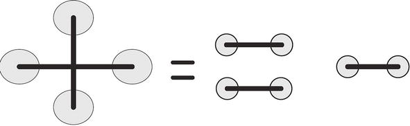
Figure 5.

In our diagrammatic analysis the right-hand side of the figure yields $1+1+1=3$ as the entanglement of formation, being the sum of three 2-qubit entanglements. Thus, in our diagrammatic analysis, we obtained exact equality not inequality.

This sort of diagrammatic analysis of the entropy of entanglement of formation can straightforwardly be employed to all multi-partite qubit systems by a simple counting argument as is done here. For example, for 18 multi-partite entangled qubits in Figure 6, we have the entanglement of formation schematically depicted by the equality where there is 17 number of monogamy in the right-hand side yielding 17 qubits of entropy of entanglement of formation.

Figure 6.

In our diagrammatic analysis the right hand side of the figure yields $1+1+1,.\dots \mathrm{..1}=17$ qubits as the entanglement of formation, being the sum of 17 two-qubit entanglements of formation. There are 18 multi-party entangled qubits in the left-hand side.

7. Joint distributions as entanglements

In this section, we will explicitly show the discrete phase-space physics of qubit entanglements. We will demonstrate that a joint “Bloch-function” distributions in “momentum space” transforms into entangled qubits (“Wannier states”) in “lattice-site space”⁴. To the author’s knowledge, this demonstrates for the first time the entanglement properties of joint distributions in quantum mechanics, which is ubiquitous in quantum transport theory of topological insulators discussed in Ref. [6].

Consider the generalized Fourier transformation between two Hilbert spaces,

$$\left|p\right.⟩=\sum _q\left.⟨q\right|p⟩\left|q\right.⟩,$$E60

where the $\left.⟨q\right|p⟩$ is the transformation function. This is particularly given by the discrete Fourier transform function,

$$\left.⟨q\right|p⟩=\frac{1}{\sqrt{N}}exp\left(-\frac{i}{\mathrm{\hslash }}p\cdot q\right).$$E61

where N is the number of discrete points in bijective transformations (this number N is conveniently taken as prime integers).

7.1 Two-point joint distributions

We have a joint distribution in p-space as,

$$\left|p^{\text{'}}\right.⟩\left|p^{\text{'}\text{'}}\right.⟩=\frac{1}{\sqrt{N}}\sum _{q^{\text{'}}}exp\left(-\frac{i}{\mathrm{\hslash }}{p}^{\text{'}}\cdot q^{\text{'}}\right)\left|q^{\text{'}}\right.⟩\frac{1}{\sqrt{N}}\sum _{q^{\text{'}\text{'}}}exp\left(-\frac{i}{\mathrm{\hslash }}{p}^{\text{'}\text{'}}\cdot q^{\text{'}\text{'}}\right)\left|q^{\text{'}\text{'}}\right.⟩.$$E62

Therefore, for a qubit or a two-state system, we write,

$$\left|p\right.⟩=\frac{1}{\sqrt{2}}\sum _{q=0}^{1}exp\left(-\frac{i}{\mathrm{\hslash }}p\cdot q\right)\left|q\right.⟩.$$E63

Consider the joint distribution of two qubits in “Bloch-function” space. We can form 4 joint distributions of Bloch-function in what follows. To derive these, first, we write the following matrix-representation and Hadamard-transformation identity,

$$\begin{array}{l}\pi \mathrm{\hslash }\left(\begin{array}{c}\left|0\right.⟩\\ \left|1\right.⟩\end{array}\right)\otimes \pi \mathrm{\hslash }\left(\begin{array}{c}\left|0\right.⟩\\ \left|1\right.⟩\end{array}\right)\\ =\frac{1}{\sqrt{2}}\frac{1}{\sqrt{2}}\left(\begin{array}{c}\left(\left|0\right.⟩+\left|1\right.⟩\right)\\ \left(\left|0\right.⟩-\left|1\right.⟩\right)\end{array}\right)\otimes \left(\begin{array}{c}\left(\left|0\right.⟩+\left|1\right.⟩\right)\\ \left(\left|0\right.⟩-\left|1\right.⟩\right)\end{array}\right).\end{array}$$E64

We will denote the joint distribution in p-space as $\mathcal{D}\left(p_1,p_2,.\dots ,p_n\right)$. We will denote these 4 “Bloch-function” distributions by the standard notations for the Bell basis in the literature, namely, ${\mathrm{\Phi }}^{+},$ ${\mathrm{\Phi }}^{-},{\mathrm{\Psi }}^{+}$ and ${\mathrm{\Psi }}^{-}$. Then, we have

$$\mathcal{D}\left(0,0\right)=\frac{1}{\sqrt{2}}\left\{{\mathrm{\Phi }}^{+}+{\mathrm{\Psi }}^{+}\right\},\mathcal{D}\left(1,1\right)=\frac{1}{\sqrt{2}}\left({\mathrm{\Phi }}^{+}-{\mathrm{\Psi }}^{+}\right),$$E65

$$\mathcal{D}\left(0,1\right)=\frac{1}{\sqrt{2}}\left({\mathrm{\Phi }}^{-}-{\mathrm{\Psi }}^{-}\right),\mathcal{D}\left(1,0\right)=\frac{1}{\sqrt{2}}\left({\mathrm{\Phi }}^{-}+{\mathrm{\Psi }}^{-}\right).$$E66

7.2 Three-point joint distributions

Similarly, for three-fold joint distribution in p-space, we have,

$$\begin{array}{lll}\left|p_1\right.⟩\left|p_2\right.⟩\left|p_3\right.⟩& =& \frac{1}{\sqrt{N}}\sum _{q_1}exp\left(-\frac{i}{\mathrm{\hslash }}{p}_1\cdot q_1\right)\left|q_1\right.⟩\\ & & \times \frac{1}{\sqrt{N}}\sum _{q_2}exp\left(-\frac{i}{\mathrm{\hslash }}{p}_2\cdot q_2\right)\left|q_2\right.⟩\\ & & \times \frac{1}{\sqrt{N}}\sum _{q_3}exp\left(-\frac{i}{\mathrm{\hslash }}{p}_3\cdot q_3\right)\left|q_3\right.⟩.\end{array}$$E67

Again, in matrix form, we express the above equation as

$$\begin{array}{l}\pi \mathrm{\hslash }\left(\begin{array}{c}\left|0\right.⟩\\ \left|1\right.⟩\end{array}\right)\otimes \pi \mathrm{\hslash }\left(\begin{array}{c}\left|0\right.⟩\\ \left|1\right.⟩\end{array}\right)\otimes \pi \mathrm{\hslash }\left(\begin{array}{c}\left|0\right.⟩\\ \left|1\right.⟩\end{array}\right)\\ =\frac{1}{\sqrt{2}}\left(\begin{array}{cc}1& 1\\ 1& -1\end{array}\right)\left(\begin{array}{c}\left|0\right.⟩\\ \left|1\right.⟩\end{array}\right)\otimes \frac{1}{\sqrt{2}}\left(\begin{array}{cc}1& 1\\ 1& -1\end{array}\right)\left(\begin{array}{c}\left|0\right.⟩\\ \left|1\right.⟩\end{array}\right)\otimes \frac{1}{\sqrt{2}}\left(\begin{array}{cc}1& 1\\ 1& -1\end{array}\right)\left(\begin{array}{c}\left|0\right.⟩\\ \left|1\right.⟩\end{array}\right),\\ =\frac{1}{\sqrt{2}}\frac{1}{\sqrt{2}}\frac{1}{\sqrt{2}}\left(\begin{array}{c}\left(\left|0\right.⟩+\left|1\right.⟩\right)\\ \left(\left|0\right.⟩-\left|1\right.⟩\right)\end{array}\right)\otimes \left(\begin{array}{c}\left(\left|0\right.⟩+\left|1\right.⟩\right)\\ \left(\left|0\right.⟩-\left|1\right.⟩\right)\end{array}\right)\otimes \left(\begin{array}{c}\left(\left|0\right.⟩+\left|1\right.⟩\right)\\ \left(\left|0\right.⟩-\left|1\right.⟩\right)\end{array}\right).\end{array}$$E68

From Eq. (68), we can define 8 joint distributions in p-space, namely, $\mathcal{D}\left(\mathrm{0,0,0}\right)$, $\mathcal{D}\left(\mathrm{0,0,1}\right)$, $\mathcal{D}\left(\mathrm{0,1,0}\right)$, $\mathcal{D}\left(\mathrm{0,1,1}\right)$, $\mathcal{D}\left(\mathrm{1,0,0}\right)$, $\mathcal{D}\left(\mathrm{1,0,1}\right)$, $\mathcal{D}\left(\mathrm{1,1,0}\right)$, and $\mathcal{D}\left(\mathrm{1,1,1}\right)$. We obtained,

$$\mathcal{D}\left(\mathrm{0,0,0}\right)=\frac{1}{\sqrt{4}}\left\{\left({\mathrm{\Theta }}_3^{+}+{\mathrm{\Gamma }}^{+}+{\mathrm{\Xi }}^{+}+{\mathrm{\Omega }}^{+}\right)\right\},$$E69

$$\mathcal{D}\left(\mathrm{0,0,1}\right)=\frac{1}{\sqrt{4}}\left\{\left({\mathrm{\Theta }}_3^{-}+{\mathrm{\Gamma }}^{-}+{\mathrm{\Xi }}^{-}+{\mathrm{\Omega }}^{-}\right)\right\},$$E70

$$\mathcal{D}\left(\mathrm{0,1,0}\right)=\frac{1}{\sqrt{4}}\left\{{\mathrm{\Theta }}_3^{-}-{\mathrm{\Xi }}^{-}+{\mathrm{\Gamma }}^{-}-{\mathrm{\Omega }}^{-}\right\},$$E71

$$\mathcal{D}\left(\mathrm{0,1,1}\right)=\frac{1}{\sqrt{4}}\left\{{\mathrm{\Theta }}_3^{+}-{\mathrm{\Gamma }}^{+}-{\mathrm{\Omega }}^{+}+{\mathrm{\Xi }}^{+}\right\},$$E72

$$\mathcal{D}\left(\mathrm{1,0,0}\right)=\frac{1}{\sqrt{4}}\left\{{\mathrm{\Theta }}_3^{-}+{\mathrm{\Omega }}^{-}+{\mathrm{\Gamma }}^{-}+{\mathrm{\Xi }}^{-}\right\},$$E73

$$\mathcal{D}\left(\mathrm{1,0,1}\right)=\frac{1}{\sqrt{4}}\left\{{\mathrm{\Theta }}_3^{+}-{\mathrm{\Xi }}^{+}+{\mathrm{\Omega }}^{+}-{\mathrm{\Gamma }}^{+}\right\},$$E74

$$\mathcal{D}\left(\mathrm{1,1,0}\right)=\frac{1}{\sqrt{4}}\left\{{\mathrm{\Theta }}_3^{+}-{\mathrm{\Xi }}^{+}-{\mathrm{\Omega }}^{+}+{\mathrm{\Gamma }}^{+}\right\},$$E75

$$\mathcal{D}\left(\mathrm{1,1,1}\right)=\frac{1}{\sqrt{4}}\left\{{\mathrm{\Theta }}_3^{-}+{\mathrm{\Xi }}^{-}-{\mathrm{\Omega }}^{-}-{\mathrm{\Gamma }}^{-}\right\}.$$E76

In Eqs. (69)–(76), we made use of the following relations:

$$\frac{1}{\sqrt{2}}\left(\left|0\right.⟩\left|0\right.⟩\left|0\right.⟩+\left|1\right.⟩\left|1\right.⟩\left|1\right.⟩\right)={\mathrm{\Theta }}_3^{+},\frac{1}{\sqrt{2}}\left(\left|0\right.⟩\left|0\right.⟩\left|1\right.⟩+\left|1\right.⟩\left|1\right.⟩\left|0\right.⟩\right)={\mathrm{\Gamma }}^{+},$$E77

$$\frac{1}{\sqrt{2}}\left(\left|0\right.⟩\left|1\right.⟩\left|0\right.⟩+\left|1\right.⟩\left|0\right.⟩\left|1\right.⟩\right)={\mathrm{\Omega }}^{+},\frac{1}{\sqrt{2}}\left(\left|0\right.⟩\left|1\right.⟩\left|1\right.⟩+\left|1\right.⟩\left|0\right.⟩\left|0\right.⟩\right)={\mathrm{\Xi }}^{+},$$E78

$$\frac{1}{\sqrt{2}}\left(\left|0\right.⟩\left|0\right.⟩\left|0\right.⟩-\left|1\right.⟩\left|1\right.⟩\left|1\right.⟩\right)={\mathrm{\Theta }}_3^{-},\frac{1}{\sqrt{2}}\left(\left|0\right.⟩\left|0\right.⟩\left|1\right.⟩-\left|1\right.⟩\left|1\right.⟩\left|0\right.⟩\right)={\mathrm{\Gamma }}^{-},$$E79

$$\frac{1}{\sqrt{2}}\left(\left|0\right.⟩\left|1\right.⟩\left|0\right.⟩-\left|1\right.⟩\left|0\right.⟩\left|1\right.⟩\right)={\mathrm{\Omega }}^{-},\frac{1}{\sqrt{2}}\left(\left|0\right.⟩\left|1\right.⟩\left|1\right.⟩-\left|1\right.⟩\left|0\right.⟩\left|0\right.⟩\right)={\mathrm{\Xi }}^{-}.$$E80

A crucial observation is that only even $\left(+\right)$ combinations of entangled basis states correspond to joint distributions and entanglements, and similarly only odd $\left(-\right)$ combinations of entangled basis states correspond to joint distributions and entanglements as well. This claim will become clear when we discuss the basic characterization of entanglements and of entanglement measure, which have concurrency⁵ equals 1.

8. Chiral degrees of freedom and entangled qubits

Observe that the pseudo-spin variables in semiconductor Bloch equation is defined by the following expressions,

$$S_0={\rho }_{\mathit{cc}}+{\rho }_{\mathit{vv}},$$E81

$$S_x={\rho }_{\mathit{vc}}+{\rho }_{\mathit{cv}},$$E82

$$S_y=-i\left({\rho }_{\mathit{vc}}-{\rho }_{\mathit{cv}}\right),$$E83

$$S_z={\rho }_{\mathit{cc}}-{\rho }_{\mathit{vv}}.$$E84

This maps to

$$e_0=\left|{\mathrm{\Phi }}^{+}\right.⟩=\frac{1}{\sqrt{2}}\left(\left|1\right.⟩\left|1\right.⟩+\left|0\right.⟩\left|0\right.⟩\right),$$E85

$$e_x=\left|{\mathrm{\Psi }}^{+}\right.⟩=\frac{1}{\sqrt{2}}\left(\left|0\right.⟩\left|1\right.⟩+\left|1\right.⟩\left|0\right.⟩\right),$$E86

$${\mathit{ie}}_y=i\left|{\mathrm{\Psi }}^{-}\right.⟩=\frac{1}{\sqrt{2}}\left(\left|0\right.⟩\left|1\right.⟩-\left|1\right.⟩\left|0\right.⟩\right),$$E87

$$e_z=\left|{\mathrm{\Phi }}^{-}\right.⟩=\frac{1}{\sqrt{2}}\left(\left|1\right.⟩\left|1\right.⟩-\left|0\right.⟩\left|0\right.⟩\right).$$E88

We refer to the basis $\left(e_0,e_x,e_y,e_z\right)$ as the pseudo-spin component basis, which differ from the Bell basis in $\left|{\mathrm{\Psi }}^{-}\right.⟩$ by the factor i in $\left|{\mathrm{\Psi }}^{-}\right.⟩$. An important observation that follows from this is that the entangling of chiral degrees of freedom creates another chiral degrees of freedom, e.g., Eqs. (69)–(76).

This is a very important observation which will aid in understanding the entanglement-induced delocalization, in topological insulators treated by the quantum transport approach in Ref. [6].

9. The concurrence concept and emergent qubit

By virtue of our diagrammatic construction, coupled with discrete phase space Hadamard transformation, in deriving the entangled basis states, the concurrence concept defined by Wooters [2, 3], as well as the two-state (qubit) properties of entangled multi-partite qubits, naturally coincides with the mathematical description of our physical model of qubit entanglement. In other words, the essence of the quantum description of an entangled qubits in Figure 1 consists of the superposition of product ‘site states’ and their corresponding translated ‘site states’ of all qubits. This means a superposition of the two states of the entangled two qubits of Figure 1. One observe that irrespective of how many qubits are entangled, the resulting entangled state is an emergent two-state system and therefore behave just like one qubit with two-states, namely, the first state and its translated state [4]. Therefore its associated entropy is just one⁶.

The concept of concurrence is basically contained by construction of our physical model of qubit entanglement. It is defined by

$$\left|\left.⟨\mathrm{\Psi }\right|\left|\tilde{\mathrm{\Psi }}\right.⟩\right|=C,$$E89

where C is the quantitative value of concurrence. This number lies between 0 and 1, 0 $\le C\le$ 1. Here $\tilde{\mathrm{\Psi }}$ is the corresponding translated qubits of $\mathrm{\Psi }$.

10. A natural measure of entanglement

The two properties of any entangled qubits, namely, concurrence and its emergent qubit behavior, lead Wooters [2, 3] to introduce a measure of entanglement, as incorporated in the two formulas,

$$E\left(C\right)=H\left(\frac{1}{2}+\frac{1}{2}\sqrt{1-C^2}\right),$$E90

$$H\left(x\right)=-xlnx-\left(1-x\right)ln\left(1-x\right).$$E91

Equation (90) basically say that if there is complete concurrence, i.e., $C=1$, then Eq. (91) says that the system behave as an emergent qubit or two-state system, as depicted clearly in our diagrams. Thus, for maximally entangled multi-partite qubits, we have $C=1$,

$$E\left(C\right)=H\left(\frac{1}{2}\right),$$E92

$$H\left(\frac{1}{2}\right)=\frac{1}{2}ln2+\frac{1}{2}ln2,=1.$$E93

affirming that entangled qubits behave as a two-state system or as an emergent qubit, yielding entropy equals one.

10.1 Entropic distance in entanglement measure

From the above developments, one can introduce an entanglement entropic distance by the formula

$$\mathrm{ℰ}=\left|\mathit{Tr}\left(\rho ln\rho \right)-1\right|,$$E94

where $\mathit{Tr}\left(\rho ln\rho \right)$ is evaluated using Eqs. (90) and (91). This distance has a range: $0\le \mathrm{ℰ}\le 1.$ When the concurrence, $C=1$, $\mathit{Tr}\left(\rho ln\rho \right)=1=H\left(\frac{1}{2}\right)$, then we have the entropy-distance from maximally entangled state, $\mathrm{ℰ}=0$. When $C=0$, $\mathit{Tr}\left(\rho ln\rho \right)=0=H\left(1\right)$, then we have the entropy-distance from maximally entangled state, $\mathrm{ℰ}=1$.

An example where the $C<1$ may occur in the following singlet state, with less entanglement,

$$\left|\psi \right.⟩=\alpha \left|01\right.⟩+\beta \left|10\right.⟩,$$E95

where

$${\alpha }^2+{\beta }^2=1.$$E96

Then

$$\begin{array}{lll}C& =& \left|\left.⟨\psi \right|\left|\tilde{\psi }\right.⟩\right|=\left(\alpha \left.⟨01\right|+\beta \left.⟨10\right|\right)\left(\alpha \left|10\right.⟩+\beta \left|01\right.⟩\right),\\ & =& \mathit{\alpha \beta }+\mathit{\beta \alpha }\le 1.\end{array}$$E97

11. Mixed states and pure states

In discussing mixed and pure states, one makes use of density-matrix operators. This is the domain of abstract statistical treatment usually found in the literature, perhaps following the statistical tradition of Bell’s theorem. To elucidate the basic physics, we will here avoid abstract statistical treatment and only discuss specific situations and examples.

11.1 Mixed states and mixed entanglements

Consider the maximally mixed state of a triplet system,

$${\widehat{\rho }}_W=\frac{1}{2}\left(\left|00\right.⟩\left.⟨00\right|+\left|11\right.⟩\left.⟨11\right|\right).$$E98

We obtain the mixed entanglements given by,

$${\widehat{\rho }}_B=\frac{1}{2}\left(\left|{\mathrm{\Phi }}^{+}{\mathrm{\Phi }}^{+}\right.⟩\left.⟨{\mathrm{\Phi }}^{+}{\mathrm{\Phi }}^{+}\right|+\left|{\mathrm{\Phi }}^{-}{\mathrm{\Phi }}^{-}\right.⟩\left.⟨{\mathrm{\Phi }}^{-}{\mathrm{\Phi }}^{-}\right|\right).$$E99

Similarly, consider the maximally mixed state of a singlet system,

$${\widehat{\rho }}_W=\frac{1}{2}\left(\left|01\right.⟩\left.⟨01\right|+\left|10\right.⟩\left.⟨10\right|\right).$$E100

We obtain the mixed entanglements given by

$${\widehat{\rho }}_B=\frac{1}{2}\left(\left|{\mathrm{\Psi }}^{+}{\mathrm{\Psi }}^{+}\right.⟩\left.⟨{\mathrm{\Psi }}^{+}{\mathrm{\Psi }}^{+}\right|+\left|{\mathrm{\Psi }}^{-}{\mathrm{\Psi }}^{-}\right.⟩\left.⟨{\mathrm{\Psi }}^{-}{\mathrm{\Psi }}^{-}\right|\right).$$E101

11.2 Mixed state from pure state (entangled state)

Consider the example of a bipartite of two qubit system. Consider a pure entangled state,

$$\left|\psi \right.⟩=\frac{1}{\sqrt{2}}\left(\left|00\right.⟩+\left|11\right.⟩\right).$$E102

Then the density matrix is,

$$\rho =\frac{1}{2}\left(\left|00\right.⟩+\left|11\right.⟩\right)\left(\left.⟨00\right|+\left.⟨11\right|\right),$$E103

where the first qubit belongs to party A and the second qubit belongs to party B.⁷ We have

$${\rho }^2=\rho ,$$E104

so that Eq. (103) is a pure state. Again, we have, by tracing the party B we obtain,

$$\begin{array}{lll}{\rho }_A& =& {\mathit{Tr}}_B\rho ,\\ & =& \frac{1}{2}\left(\left|0_A\right.⟩\left.⟨0_A\right|+\left|1_A\right.⟩\left.⟨1_A\right|\right).\end{array}$$E105

Now clearly

$${\rho }_A^2=\frac{1}{2}{\rho }_A,$$E106

so that ${\rho }_A$ is not a pure state but mixed, i.e., a mixture of two pure states, $\left|0_A\right.⟩$ and $\left|1_A\right.⟩$.⁸ Note that the mixed states density matrix do not possess off-diagonal elements. The tracing operation basically eliminates the contribution of the “off-diagonal” terms. From the last identity, the eigenvalues of ${\rho }_A$ is $\frac{1}{2}$ and since the subsystem A is an emergent qubit, in general with two distinct states, then eigenvalues of ${\rho }_A$ corresponds to $\frac{1}{\mathrm{\Omega }}$ of our first example above. Thus we refer to ${\rho }_A$ as “uniformly’” mixed often referred to as “maximally mixed” with the initial state $\left|\psi \right.⟩$ as “maximally entangled”.

12. Concluding remarks

The inverter-chain rigid-coupling mechanical model of entanglement link has been demonstrated to faithfully implement the discrete phase space viewpoint [4]. The crucial observation that arise from this inverter-chain link model is that any multi-partite qubit entangled system has the property of an emergent qubit, which has been rigorously justified. This readily lead us to the equality relations of the entropy of entanglement formation in the so-called monogamy inequality of entanglement formation, using statistical arguments [5] discussed in the literature. In this paper, mixed states and mixed entanglements are related by the Hadamard transformations [7]. In addition, we show that mixed state can be extracted from pure entangled state, where the party A or B need not be a single qubit themselves but can each be an entangled multi-partite qubit system, respectively, by virtue of emergent qubit property of entangled qubit systems. We find that joint distributions in quantum mechanics have inherent entanglement properties.

The natural measure of entanglement is based on entropy of entanglement formation, concurrence, and entropic distance from maximally entangled reference.

References

- 1.
Einstein A, Podolsky B, Rosen N. Can quantum-mechanical description of physical reality be considered complete? Physics Review. 1935; 47 :777 - 2.
Hill S, Wooters WK. Entanglement of a pair of quantum bits. Physical Review Letters. 1977; 78 :5022 - 3.
Wooters WK. Entanglement of a pair of quantum bits. Physical Review Letters. 1998; 80 :2245 - 4.
Buot FA, Elnar AR, Maglasang G, Galon CM. A mechanical implementation and diagrammatic calculation of entangled basis states. arXiv:2112.10291 [cond-mat.mes-hall]. 2021 - 5.
Kim JS. Entanglement of formation and monogamy of multi-party quantum entanglement. Scientific Reports. 2021; 11 :2364. DOI: 10.1038/s41598-021-82052-3 - 6.
Buot FA, Rivero KB, Otadoy RES. Generalized nonequilibrium quantum transport of spin and pseudospins: Entanglements and topological phases. Physica B. 2019; 559 :42-61 - 7.
Buot FA. Nonequilibrium Quantum Transport Physics in Nanosystem. Hackensack, NJ, USA: World Scientific; 2009, and references therein
Notes
- Note that although Bell’s theorem asserts the nonlocality of quantum mechanics, the EPR inquiry is still not resolved, i.e., what is still left unanswered is the mysterious ‘link’ between qubits corresponding to our “see-saw” or mechanical inverter-chain link. (Note: Bell’s inequality theorem is widely discussed in the literature and websites, we prefer not to cite specific reference).
- The use of the term “triplet” is actually a misnomer here since the entangled system is not free to assume a singlet or zero spin state. Thus, this term is used here only as a label.
- The idea that entanglement is due to conservation of momentum does not hold for triplet entanglement since its two states give opposing spin-angular momentum. However, one may interpret that quantum superposition of the two-opposing angular momentum states conserves the overall zero net spin-angular momentum, as supported by their eigenvalues similar to a single qubit. On the other hand, for singlet entanglement, the zero angular momentum is conserve in both two states. This seemingly apparent physical difference of the triplet and singlet entanglements underscores the importance of resolving the “mysterious link” in the EPR inquiry, [1] in order to further advance theoretical physics.
- We maintained the Bloch function/Wannier function analogy for convenience, and to stress the wide-ranging impact of the discrete phase-space physics.
- Concurrency is one of the most important characterization of entangled qubits, to be discussed in more details below.
- This is also deduced when concurrence C=1 [3].
- What we mean by party A and B is in the general sense since any entangled number of qubits behave as an emergent qubit.
- If the parties A and B are entangled states, then what we have obtain are also mixed entanglement through the inverse Hadamard transformation.