Translational Symmetry of Intermediate Nodes and Antinodes of Entangled Particles

Abstract

In a 1935 publication, Albert Einstein, Boris Podolsky, and Nathan Rosen present a thought experiment meant to demonstrate the apparent absurdity of quantum entanglement, which appeared to be in direct opposition to a fundamental law of the world. It was obvious to the men who created quantum mechanics in the decade of 1920, that quantum entanglement is unsettling because of the fact that quantum superposition is a real phenomenon. Thomas Vidick, a professor of physics, says it may be alluring to believe that the particles are somehow interacting with each other across such vast distances. A key resource for quantum networks is entanglement, a fundamental aspect of quantum theory that enables the sharing of unbreakable quantum connections between distant participants. Distributing entanglement across distant items that can act as quantum memory is very important. This has been accomplished in the past employing systems like warm and cold atomic vapours, single atoms and ions, and flaws in solid-state system

1. Introduction

Einstein splendidly criticised the phenomenon of quantum physics, particularly quantum entanglement, which shows how particles can share a combined state while separated arbitrarily far apart. Struggling with the oddity of this phenomenon, he referred to it as “spooky action at a distance” [1, 2]. This uncertainty has recently become more pronounced in various non-locality forms. The truth of this phenomenon has recently been confirmed by scientists over ever-greater distances, even from Earth to an orbiting spacecraft. Many times, it defies the special theory of relativity’s fundamental tenet that nothing can move faster than the speed of light, which has baffled scientists for years. In this study, the author suggests a potential quantum entanglement mechanism that upholds the special theory’s basic premise. It is important to note that the spin directions of the entangled particles such as vector bosons in Higgs boson decays are comparable to the corresponding phases of the standing wave’s intermediate field particles. Furthermore, a crucial phenomenon known as “phase transitions” can be observed in one-dimensional overlaid mixed wave functions. A crucial finding is that the application of a magnetic field to any entangled particle, no matter how minute, results in the same spin orientations in the intermediate antinodes regardless of temperature changes.

By effectively splitting a system into two parts, where the sum of the portions is known, entangled particles are produced. For instance, it is possible to divide a particle with spin zero into two particles whose spins will inevitably be opposite one another, resulting in a sum of zero.

David Bohm is credited with coming up with a condensed version of this thought experiment that takes the decay of the pi meson into account. The electron and positron that are created when this particle decays have opposite spins and are travelling away from one another. So, if the measured spin of the electron is up, the measured spin of the positron can only be down, and the opposite is true. Even if the particles are billions of miles distant, this is still true.

If the measured positron spin were always down and the measured electron spin were always up, everything would be OK. Each particle’s spin, however, has both an up and a down component until it is detected due to quantum physics. The quantum state of the spin does not “collapse” into either up or down until the measurement takes place, at which point the other particle instantly assumes the opposite spin. This appears to indicate that the particles are in communication with one another via a method that is moving faster than light. However, nothing can move more quickly than the speed of light, according to the laws of physics. Undoubtedly, it is impossible to instantly predict the state of one particle from its measured condition.

A formula created by Bell is now known as Bell’s inequality, and it is only and always true for hidden variable theories—never for quantum mechanics. This means that local hidden variable theories cannot account for quantum entanglement if Bell’s equation is proven to be unsatisfied in a real-world experiment. The idea that entangled particles are communicating with one another faster than the speed of light contradicts Einstein’s special theory of relativity, and is a popular fallacy about entanglement. This is not the case, and quantum physics cannot be employed to deliver messages that travel at a faster-than-light rate. The origin of the entanglement phenomena, which at first glance appears strange, is still a topic of controversy among scientists, but they are aware that the theory behind it holds up to repeated testing. Despite the fact that Einstein famously called entanglement “spooky action at a distance,” modern quantum scientists assert that it is not spooky in any way. According to Schrödinger, with a certain probability, a particle in another location could be guided into one of a set of states by an entangled state. In reality, the ‘remote guiding’ potential is considerably more spectacular than Schrödinger’s experiment. Assuming, two experimenter Bob and Alice both possess a pair of entangled photons that are in an entangled pure state similar to those Bell considered, with Alice possessing one of the entangled photons and Bob is holding the other. Assume that Alice also receives an additional photon with unknown polarisation $\left|a\right.⟩$ where “$\left|\right.⟩$” represents a quantum state. If Alice performs an operation on the two photons in her possession, Bob’s photon may change into one of the four states. The four possible (random) outcomes of Alice’s operation are either the state $\left|a\right.⟩$ or a state that is clearly related to $\left|a\right.⟩$. The two photons Alice is holding become entangled as a result of Alice’s operation, which also manages to separate Bob’s photon and direct it into a state of $\left|a^{\ast }\right.⟩$. Bob is either aware that $\left|a^{\ast }\right.⟩=\left|a\right.⟩$ or understands how to do a local operation to change $\left|a^{\ast }\right.⟩\text{to}\left|a\right.⟩$ after Alice tells him the results of her operation. Quantum teleportation is the term used to describe this phenomenon. Both Alice and Bob are unable to determine the state $\left|a\right.⟩$ following the teleportation technique [3, 4]. Two conventional bits of information can be used to specify Alice’s operation’s result, which has four potential outcomes and an equal probability of 0.25. Surprisingly, Bob can recreate the state $\left|a\right.⟩$ from just two bits of classical information that Alice has communicated. It appears that Bob did this by using the entangled state as a quantum communication channel. The noteworthy aspect of these phenomena is that Alice and Bob were able to use their shared entangled state as a quantum communication channel to alter the state $\left|a\right.⟩$ of a photon in Alice’s part of the universe and reproduce it in Bob’s portion of the universe.

In 1989, Daniel Greenberger, Michael Horne, and Anton Zeilinger conducted the initial research on it. A Greenberger-Horne-Zeilinger state (GHZ state) is a specific kind of entangled quantum state in the field of quantum information theory that involves three subsystems (particle states, qubits, or qudits). In advancement of this aforesaid theory on the year 2020, Kisalaya Chakrabarti proposed an entangled quantum state in the field of quantum information theory that involves four subsystems called Kisalaya state (K state) [4].

In this regard, it is worth mentioning, aground-breaking workshop that was held at the Brookhaven National Laboratory in 2018, from onwards the ideas of using quantum information methods and tools in high-energy physics is gaining more and more attention. We know that, the density matrix of the hadrons – the bound states of quarks and gluons, must be averaged over the phase with the associated Haar integration measure because it is impossible to detect the phase of the wave function in high energy interactions. This results in the density matrix of the Parton model, which is a mixed state density matrix that is diagonal in Parton number. With the help of this method, one can better grasp the limits of the Parton model, such as how it cannot accurately describe spin-dependent processes [5].

2. Probability transfer matrix of an entangled particle at a distance

Mixed state states are possible for quantum mechanical systems. The term “pure state” refers to the states that wave functions describe. In this case, the probability states are superimposed. Starting from the Pauli’s matrix of quantum physics, which accounts for the interaction between a particle’s spin and an external electromagnetic field and additionally they depict the interaction states of two polarisation filters for 45° right or left, circular or horizontal or vertical polarisation, given by:

$${\sigma }_x=\left[\begin{array}{cc}0& 1\\ 1& 0\end{array}\right],{\sigma }_y=\left[\begin{array}{cc}0& -i\\ i& 0\end{array}\right]\text{and}{\sigma }_z=\left[\begin{array}{cc}1& 0\\ 0& -1\end{array}\right]$$

Now, taking the tensor products of two parallel operations at superimposed similar states given as follows;

$${\sigma }_x\otimes {\sigma }_x=\left[\mathrm{A}\right]=\left[\begin{array}{cc}0& 1\\ 1& 0\end{array}\right]\left[\begin{array}{cc}0& 1\\ 1& 0\end{array}\right]=\left[\begin{array}{cccc}0& 0& 0& 1\\ 0& 0& 1& 0\\ 0& 1& 0& 0\\ 1& 0& 0& 0\end{array}\right]=\left[\begin{array}{cccc}{\rho }_i& {\rho }_i& {\rho }_i& 1-{\rho }_i\\ {\rho }_i& {\rho }_i& 1-{\rho }_i& {\rho }_i\\ {\rho }_i& 1-{\rho }_i& {\rho }_i& {\rho }_i\\ 1-{\rho }_i& {\rho }_i& {\rho }_i& {\rho }_i\end{array}\right]$$E1

Instead of using wave functions in this situation, we must employ the idea of a probability transfer matrix. A mixed state can be represented as an incoherent summation of Orthonormal bases $\left|{\psi }_i\right.⟩$‘s as $\rho =\sum _i{\rho }_i\left|{\psi }_i\right.⟩\left.⟨{\psi }_i\right|$ where ${\rho }_i$ is the probability $P$ for the system in the state of ${\psi }_i$, and ${\psi }_i$‘s are the diagonal basis for $\rho$. ${\rho }_i$ are referred to as the density matrix’s Eigen values $\rho$.

Similarly,

$$\begin{array}{lll}{\sigma }_y\otimes {\sigma }_y& =& \left[\mathrm{B}\right]=\left[\begin{array}{cc}0& -i\\ i& 0\end{array}\right]\left[\begin{array}{cc}0& -i\\ i& 0\end{array}\right]=\left[\begin{array}{cccc}0& 0& 0& -1\\ 0& 0& +1& 0\\ 0& +1& 0& 0\\ -1& 0& 0& 0\end{array}\right]\\ & =& \left[\begin{array}{cccc}{\rho }_i& {\rho }_i& {\rho }_i& \left|{\rho }_i-1\right|\\ {\rho }_i& {\rho }_i& 1-{\rho }_i& {\rho }_i\\ {\rho }_i& 1-{\rho }_i& {\rho }_i& {\rho }_i\\ \left|{\rho }_i-1\right|& {\rho }_i& {\rho }_i& {\rho }_i\end{array}\right]\end{array}$$E2

and

$$\begin{array}{lll}{\sigma }_z\otimes {\sigma }_z& =& \left[\mathrm{C}\right]=\left[\begin{array}{cc}1& 0\\ 0& -1\end{array}\right]\left[\begin{array}{cc}1& 0\\ 0& -1\end{array}\right]=\left[\begin{array}{cccc}1& 0& 0& 0\\ 0& -1& 0& 0\\ 0& 0& -1& 0\\ 0& 0& 0& 1\end{array}\right]\\ & =& \left[\begin{array}{cccc}1-{\rho }_i& {\rho }_i& {\rho }_i& {\rho }_i\\ {\rho }_i& \left|{\rho }_i-1\right|& {\rho }_i& {\rho }_i\\ {\rho }_i& {\rho }_i& \left|{\rho }_i-1\right|& {\rho }_i\\ {\rho }_i& {\rho }_i& {\rho }_i& 1-{\rho }_i\end{array}\right]\end{array}$$E3

Tensor Products or Tensor Matrices A, B and C are a set of three $4\times 4$ complex matrices which are Hermitian, involutory and unitary. Here worth mentioning that, if and only if; ${\mathrm{M}}^2=\mathrm{I}$, where I is the $4\times 4$ identity matrix, then multiplying by the matrix M results in an involution. Each and every involutory matrix is the square root of the identity matrix. This is merely a result of the fact that the identity is obtained by multiplying any non-singular matrix by its inverse.

It is an important observation that none of the Tensor matrices (Tensor products) A, B and C have elements consisting of imaginary quantity. The two Eigen values of the three Hermitian Tensor products are +1 and −1.

In the same fashion one can achieve:

$$\begin{array}{lll}{\sigma }_x\otimes {\sigma }_y& =& \left[\mathrm{D}\right]=\left[\begin{array}{cc}0& 1\\ 1& 0\end{array}\right]\left[\begin{array}{cc}0& -i\\ i& 0\end{array}\right]=\left[\begin{array}{cccc}0& 0& 0& -i\\ 0& 0& i& 0\\ 0& -i& 0& 0\\ i& 0& 0& 0\end{array}\right]\\ & =& i\left[\begin{array}{cccc}{\rho }_i& {\rho }_i& {\rho }_i& \left|{\rho }_i-1\right|\\ {\rho }_i& {\rho }_i& 1-{\rho }_i& {\rho }_i\\ {\rho }_i& \left|{\rho }_i-1\right|& {\rho }_i& {\rho }_i\\ 1-{\rho }_i& {\rho }_i& {\rho }_i& {\rho }_i\end{array}\right]\end{array}$$E4

$$\begin{array}{lll}{\sigma }_y\otimes {\sigma }_z& =& \left[\mathrm{E}\right]=\left[\begin{array}{cc}0& -i\\ i& 0\end{array}\right]\left[\begin{array}{cc}1& 0\\ 0& -1\end{array}\right]=\left[\begin{array}{cccc}0& 0& -i& 0\\ 0& 0& 0& i\\ i& 0& 0& 0\\ 0& -i& 0& 0\end{array}\right]\\ & =& i\left[\begin{array}{cccc}{\rho }_i& {\rho }_i& \left|{\rho }_i-1\right|& {\rho }_i\\ {\rho }_i& {\rho }_i& {\rho }_i& 1-{\rho }_i\\ 1-{\rho }_i& {\rho }_i& {\rho }_i& {\rho }_i\\ {\rho }_i& \left|{\rho }_i-1\right|& {\rho }_i& {\rho }_i\end{array}\right]\end{array}$$E5

$${\sigma }_z\otimes {\sigma }_x=\left[\mathrm{F}\right]=\left[\begin{array}{cc}1& 0\\ 0& -1\end{array}\right]\left[\begin{array}{cc}0& 1\\ 1& 0\end{array}\right]=\left[\begin{array}{cccc}0& 1& 0& 0\\ 1& 0& 0& 0\\ 0& 0& 0& -1\\ 0& 0& -1& 0\end{array}\right]=\left[\begin{array}{cccc}{\rho }_i& 1-{\rho }_i& {\rho }_i& {\rho }_i\\ 1-{\rho }_i& {\rho }_i& {\rho }_i& {\rho }_i\\ {\rho }_i& {\rho }_i& {\rho }_i& \left|{\rho }_i-1\right|\\ {\rho }_i& {\rho }_i& \left|{\rho }_i-1\right|& {\rho }_i\end{array}\right]$$E6

In the reverse order the Tensor products are given as follows:

$$\begin{array}{lll}{\sigma }_y\otimes {\sigma }_x& =& \left[\mathrm{G}\right]=\left[\begin{array}{cc}0& -i\\ i& 0\end{array}\right]\left[\begin{array}{cc}0& 1\\ 1& 0\end{array}\right]=\left[\begin{array}{cccc}0& 0& 0& -i\\ 0& 0& -i& 0\\ 0& i& 0& 0\\ i& 0& 0& 0\end{array}\right]\\ & =& i\left[\begin{array}{cccc}{\rho }_i& {\rho }_i& {\rho }_i& \left|{\rho }_i-1\right|\\ {\rho }_i& {\rho }_i& \left|{\rho }_i-1\right|& {\rho }_i\\ {\rho }_i& 1-{\rho }_i& {\rho }_i& {\rho }_i\\ 1-{\rho }_i& {\rho }_i& {\rho }_i& {\rho }_i\end{array}\right]\end{array}$$E7

$${\sigma }_x\otimes {\sigma }_z=\left[\mathrm{H}\right]=\left[\begin{array}{cc}0& 1\\ 1& 0\end{array}\right]\left[\begin{array}{cc}1& 0\\ 0& -1\end{array}\right]=\left[\begin{array}{cccc}0& 0& 1& 0\\ 0& 0& 0& -1\\ 1& 0& 0& 0\\ 0& -1& 0& 0\end{array}\right]=\left[\begin{array}{cccc}{\rho }_i& {\rho }_i& 1-{\rho }_i& {\rho }_i\\ {\rho }_i& {\rho }_i& {\rho }_i& \left|{\rho }_i-1\right|\\ 1-{\rho }_i& {\rho }_i& {\rho }_i& {\rho }_i\\ {\rho }_i& \left|{\rho }_i-1\right|& {\rho }_i& {\rho }_i\end{array}\right]$$E8

$$\begin{array}{lll}{\sigma }_z\otimes {\sigma }_y& =& \left[\mathrm{I}\right]=\left[\begin{array}{cc}1& 0\\ 0& -1\end{array}\right]\left[\begin{array}{cc}0& -i\\ i& 0\end{array}\right]=\left[\begin{array}{cccc}0& -i& 0& 0\\ i& 0& 0& 0\\ 0& 0& 0& i\\ 0& 0& -i& 0\end{array}\right]\\ & =& i\left[\begin{array}{cccc}{\rho }_i& \left|{\rho }_i-1\right|& {\rho }_i& {\rho }_i\\ 1-{\rho }_i& {\rho }_i& {\rho }_i& {\rho }_i\\ {\rho }_i& {\rho }_i& {\rho }_i& 1-{\rho }_i\\ {\rho }_i& {\rho }_i& \left|{\rho }_i-1\right|& {\rho }_i\end{array}\right]\end{array}$$E9

Measurements of this type are referred to as Positive operator valued measure (POVM). The most general type of POVM in which sums are substituted by integrals; so they are termed measures, which has a continuous family of outcomes. In this case there are a finite number of potential outcomes, over a finite dimensional quantum space. Hermitian matrices having finite dimensional positive operators are used here as the elements. We use these measures implicitly when we measure some qubits of a quantum computer while leaving other qubits unaffected, described in a proper mathematical definition given below:

$${\prod }_i{\prod }_j=0\text{if}i\ne j\text{and}\sum _{i-1}^k=1$$E10

Considering the case when we have a collection of projectors onto the orthogonal subspaces ${\prod }_1$, ${\prod }_2$, ….., ${\prod }_k$ which implies that the tensor products to be $\left[\mathrm{D}\right]=\left[\mathrm{E}\right]=\left[\mathrm{F}\right]=\left[\mathrm{G}\right]=\left[\mathrm{H}\right]=\left[\mathrm{I}\right]=0$, from Ortho-normality condition depicted in Eq. (10) where the projective measurement in these subspaces that evolves a quantum state $\left|\psi \right.⟩$ in the state given by

$$\left|{\psi }^{\text{'}}\right.⟩=\frac{{\prod }_{i\ne j\ne k}\left|\psi \right.⟩}{\left.⟨\psi \right|{\prod }_{i\ne j\ne k}{\left|\psi \right.⟩}^{1/2}}\text{where Probablity}P=\left.⟨\psi \right|{\prod }_{i\ne j\ne k}\left|\psi \right.⟩$$E11

A minimum rate of unresolved events or error probability $P_e$, is imposed by the state’s impossible to differentiate detection and is given by the following equation:

$$P_e=1-\mu \text{where},\mu =⟨{\psi }_i|{\psi }_j⟩$$E12

From Eq. (12) it is clearly seen that when $i\ne j$, $P_e=1$.

Therefore, the equations of importance are (1), (2) and (3) only corresponds to [A], [B} and [C] tensor product matrices where

$${\prod }_i{\prod }_i={\prod }_j{\prod }_j={\prod }_k{\prod }_k=1$$E13

Solving for Eigenvalues and Eigenvectors for [A], we find that the Eigenvalues $\lambda =\pm 1$ and the Eigenvectors are as follows:

$$\text{for}\lambda =1\text{Eigenvectors}X=\left(\begin{array}{c}{\psi }_1\\ \psi {}_2\\ {\psi }_2\\ {\psi }_1\end{array}\right)$$E14

Eq. (14) can be written as:

$$X={\psi }_1\left(\begin{array}{c}1\\ 0\\ 0\\ 1\end{array}\right)+{\psi }_2\left(\begin{array}{c}0\\ 1\\ 1\\ 0\end{array}\right)$$E15

and

$$\text{for}\lambda =-1\text{Eigenvectors}X=\left(\begin{array}{c}{\psi }_1\\ \psi {}_2\\ -{\psi }_2\\ -{\psi }_1\end{array}\right)$$E16

Eq. (16) can be written as:

$$X={\psi }_1\left(\begin{array}{c}1\\ 0\\ 0\\ -1\end{array}\right)+{\psi }_2\left(\begin{array}{c}0\\ 1\\ -1\\ 0\end{array}\right)$$E17

In the same fashion Eigenvalues and Eigenvectors for [B] are as follows:

$$\text{for}\lambda =1\text{Eigenvectors}X=\left(\begin{array}{c}{\psi }_1\\ \psi {}_2\\ {\psi }_2\\ -{\psi }_1\end{array}\right)$$E18

Eq. (18) can be written as:

$$X={\psi }_1\left(\begin{array}{c}1\\ 0\\ 0\\ -1\end{array}\right)+{\psi }_2\left(\begin{array}{c}0\\ 1\\ 1\\ 0\end{array}\right)$$E19

and;

$$\text{for}\lambda =-1\text{Eigenvectors}X=\left(\begin{array}{c}{\psi }_1\\ \psi {}_2\\ -{\psi }_2\\ {\psi }_1\end{array}\right)$$E20

Eq. (20) can be written as:

$$X={\psi }_1\left(\begin{array}{c}1\\ 0\\ 0\\ 1\end{array}\right)+{\psi }_2\left(\begin{array}{c}0\\ 1\\ -1\\ 0\end{array}\right)$$E21

Similarly, Eigenvalues and Eigenvectors for [C] are as follows:

$$\text{for}\lambda =1\text{Eigenvectors}X=\left(\begin{array}{c}{\psi }_1\\ 0\\ 0\\ {\psi }_4\end{array}\right)$$E22

Eq. (22) can be written as:

$$X={\psi }_1\left(\begin{array}{c}1\\ 0\\ 0\\ 0\end{array}\right)+{\psi }_4\left(\begin{array}{c}0\\ 0\\ 0\\ 1\end{array}\right)$$E23

and;

$$\text{for}\lambda =-1\text{Eigenvectors}X=\left(\begin{array}{c}0\\ \psi {}_2\\ {\psi }_3\\ 0\end{array}\right)$$E24

Eq. (24) can be written as:

$$X={\psi }_2\left(\begin{array}{c}0\\ 1\\ 0\\ 0\end{array}\right)+{\psi }_3\left(\begin{array}{c}0\\ 0\\ 1\\ 0\end{array}\right)$$E25

Now, from the set of two Eqs. (15) and (17); and (19) and (21) it is noticeable that only two vector states $\left|{\psi }_1\right.⟩,\left|{\psi }_2\right.⟩$ with two different orientations $\left|+,-\right.⟩$ are originated from the interference of forward and reverse moving waves at the antinodes sections resulting in Standing waves, whereas Eqs. (21) and (23) describe that presence of all the four states $\left|{\psi }_1\right.⟩,\left|{\psi }_2\right.⟩,\left|{\psi }_3\right.⟩,\left|{\psi }_4\right.⟩$ have been noticed with a single orientation $\left|+\right.⟩$. As there are only two Eigen vector states $\left|{\psi }_1\right.⟩,\left|{\psi }_2\right.⟩$ in three dimensional vector space and with two different orientations $\left|+,-\right.⟩$, it is obvious that $\left|{\psi }_4\right.⟩=-\left|{\psi }_1\right.⟩$ and $\left|{\psi }_3\right.⟩=-\left|{\psi }_2\right.⟩$.

So we can modify Eq. (23) as follows:

$$\text{for}\lambda =1X={\psi }_1\left(\begin{array}{c}1\\ 0\\ 0\\ -1\end{array}\right)$$E26

Similarly, Eq. (25) as follows and

$$\text{for}\lambda =-1X={\psi }_2\left(\begin{array}{c}0\\ 1\\ -1\\ 0\end{array}\right)$$E27

From Eqs. (15) and (17); (19) and (21) and (26) and (27) we find that only two pure states or the combination of two states are manifested with two different orientations $\left|{\psi }_{1\pm }\right.⟩,\left|{\psi }_{2\pm }\right.⟩$ at the antinodes positions due to interference of two waves originated from two entangled particles lying far apart. It is important and observed from (26) and (27) that only two pure states $\left|{\psi }_{1\pm }\right.⟩,\left|{\psi }_{2\pm }\right.⟩$ exist at antinodes at the standing wave perpendicular to the direction of propagations.

3. Entanglement theory with stationary phase approximation

Consider two entangled particles with superimposed states between them at positions “A” and “B” separated by an arbitrarily large distance “d” and having superimposed states between them ${\mathrm{\psi }}_{\mathrm{s}}$. Since there is no net energy transfers in either the forward or backward direction because the two particles are entangled, this composite wavefunction ${\mathrm{\psi }}_{\mathrm{S}}$ is composed of two $\mathrm{\psi }$ states, ${\mathrm{\psi }}_1$ and ${\mathrm{\psi }}_2$, where, ${\mathrm{\psi }}_1$ denotes the wave moving forward from “A” to “B” and a backward travelling wave ${\mathrm{\psi }}_2$ moving from “B” to “A”. The propagation of forward or backward travelling waves does not yet take the spin directions of either particle into consideration; therefore we can express the superimposed wavefunction in the context of the Schrodinger equation [4],

$${\mathrm{\psi }}_{\mathrm{S}}={\mathrm{\psi }}_1+{\mathrm{\psi }}_2=\left({\mathrm{\psi }}_{01}{\mathrm{e}}^{\frac{\mathrm{iPx}}{\mathrm{\hslash }}}+{\mathrm{\psi }}_{02}{\mathrm{e}}^{\frac{-\mathrm{iPx}}{\mathrm{\hslash }}}\right)$$E28

Without taking spin effect on directions into account, Eq. (28) can be written as

$${\mathrm{\psi }}_{\mathrm{S}}=\left({\mathrm{\psi }}_{01}{\mathrm{e}}^{\frac{\mathrm{iPx}}{\mathrm{\hslash }}}-{\mathrm{\psi }}_{01}{\mathrm{e}}^{\frac{-\mathrm{iPx}}{\mathrm{\hslash }}}\right)$$E29

Now, taking into account the spin direction of the particle at location “A” during the forward wave propagation ${\mathrm{\psi }}_1$ and we must select an axis to line up with the measuring device’s axis in order to measure the spin direction. Finally, we denote this observed spin of the particle at “A” by unit vector by moving the axis of the measurement device located at point “A” in the direction of the forward travelling wave ${\mathrm{\psi }}_1$ in the forward “+x” direction and we will denote this observed spin of the particle at point “A” by unit vector $\widehat{x}$, and bringing in this factor to “${\mathrm{\psi }}_1$” we obtained the modified wavefunction expressed as:

$${\mathrm{\psi }}_1={\mathrm{\psi }}_{01}{\mathrm{e}}^{\frac{\mathrm{iPx}}{\mathrm{\hslash }}}\widehat{x}$$E30

Taking into account the time evolution of the combined wavefunction, Eq. (29) is customised and can be written as follows:

$${\mathrm{\psi }}_{\mathrm{S}}\left(\mathrm{t}\right)=Re\left({\mathrm{\psi }}_{\mathrm{S}}{\mathrm{e}}^{\mathrm{i\omega t}}\right)=2{\mathrm{\psi }}_{01}cos\left(\frac{\mathrm{Px}}{\mathrm{\hslash }}\right)cos\left(\mathrm{\omega t}\right)\widehat{x}$$E31

where, $\mathrm{\omega }$ is the angular velocity of ${\mathrm{\psi }}_{\mathrm{S}}\left(\mathrm{t}\right),$given by $\mathrm{E}/\mathrm{\hslash }$.

It is now necessary to comprehend the stationary phase approximation of the combined wavefunction of all entangled particles, which is given by combined wave function${\mathrm{\psi }}_{\mathrm{S}}\left(\mathrm{t}\right)$, as shown in equation, in order to comprehend how quantum entanglement changes with time (31).

$$\mathrm{J}=\underset{\mathrm{\Omega }\to 0}{lim}{\int }_{-\infty }^{\infty }{\mathrm{e}}^{\mathrm{i}{\mathrm{\psi }}_{\mathrm{S}}\left(\mathrm{t}\right)/\mathrm{\Omega }}\mathrm{dt}$$E32

Eq. (32) can be stretched out as follows:

$$\mathrm{J}\approx \sum _{\mathrm{n}}{\int }_{-\infty }^{\infty }{\mathrm{e}}^{\mathrm{i}\left\{\frac{{\mathrm{\psi }}_{\mathrm{S}}\left({\mathrm{t}}_0\right)}{\mathrm{\Omega }}+\frac{\frac{\mathrm{d}{\mathrm{\psi }}_{\mathrm{S}}\left({\mathrm{t}}_0\right)}{\mathrm{dt}}\left(\mathrm{t}-{\mathrm{t}}_0\right)}{\mathrm{\Omega }}+\frac{\frac{{\mathrm{d}}^2{\mathrm{\psi }}_{\mathrm{S}}\left({\mathrm{t}}_0\right)}{\mathrm{d}{\mathrm{t}}^2}{\left(\mathrm{t}-{\mathrm{t}}_0\right)}^2}{2\mathrm{\Omega }}\right\}}\mathrm{dt}\approx {\mathrm{e}}^{\mathrm{i}\frac{{\mathrm{\psi }}_{\mathrm{S}}\left({\mathrm{t}}_0\right)}{\mathrm{\Omega }}}\sqrt{\frac{2\mathrm{\Omega \pi }}{\mathrm{i}\frac{{\mathrm{d}}^2{\mathrm{\psi }}_{\mathrm{S}}\left({\mathrm{t}}_0\right)}{\mathrm{d}{\mathrm{t}}^2}}}$$E33

In order to formally follow the convention of Gaussian integration, one should replace “i” to “-i” inside the square root portion of Eq. (33). The imaginary unit “i” is assumed to be a true positive constant even though the integral mathematically speaking does not exist. We obtain nonzero contributions precisely where, just like in the Path Integral case;

$$\mathrm{\delta }\mathrm{S}\left[{\mathrm{\psi }}_{\mathrm{S}}\left(\mathrm{t}\right),\mathrm{p}\left(\mathrm{t}\right),\mathrm{t}\right]=0$$E34

which is the prerequisite for the functional of the classical trajectory “S” and is expressed in units of$\mathrm{\hslash }$; p(t) is the momentum of the entangled system; as a result, in any physical domain where “S” is much larger than, even the slightest deviation from the classical trajectory causes ${\mathrm{\psi }}_{\mathrm{S}}\left(\mathrm{t}\right)$ to wiggle out so quickly that it has no impact on the value of “J”. The conventional boundary is $\frac{\mathrm{S}}{\mathrm{\hslash }}\gg 1$.

As is evident, that$\mathrm{J}={\mathrm{\psi }}_{\mathrm{S}}\left(\mathrm{t}\right)$, therefore squaring and comparing Eq. (31) with Eq. (33) and allowing for the real part, we obtain

$$\frac{\mathrm{\Omega \pi }sin\left(\frac{2{\mathrm{\psi }}_{\mathrm{S}}\left({\mathrm{t}}_0\right)}{\mathrm{\Omega }}\right)}{2{{\mathrm{\psi }}_{01}}^2{cos}^2\left(\mathrm{\omega t}\right)}=\frac{{\mathrm{d}}^2{\mathrm{\psi }}_{\mathrm{S}}\left({\mathrm{t}}_0\right)}{\mathrm{d}{\mathrm{t}}^2}{cos}^2\left(\frac{\mathrm{Px}}{\mathrm{\hslash }}\right)$$E35

Putting the average value of ${cos}^2\left(\frac{\mathrm{Px}}{\mathrm{\hslash }}\right)=\frac{1}{2}$ at x direction, Eq. (35) can be written as

$$\frac{\mathrm{\Omega \pi }sin\left(\frac{2{\mathrm{\psi }}_{\mathrm{S}}\left({\mathrm{t}}_0\right)}{\mathrm{\Omega }}\right)}{{{\mathrm{\psi }}_{01}}^2{cos}^2\left(\mathrm{\omega t}\right)}=\frac{{\mathrm{d}}^2{\mathrm{\psi }}_{\mathrm{S}}\left({\mathrm{t}}_0\right)}{\mathrm{d}{\mathrm{t}}^2}$$E36

Now, Eq. (36) can be rewritten as;

$$\frac{{\mathrm{d}}^2{\mathrm{\psi }}_{\mathrm{S}}\left({\mathrm{t}}_0\right)}{\mathrm{d}{\mathrm{t}}^2}=\mathrm{\kappa }\frac{sin\left({\mathrm{\psi }}_{\mathrm{S}}\left({\mathrm{t}}_0\right)\right)}{{cos}^2\left(\mathrm{\omega t}\right)}$$E37

where, $\mathrm{\kappa }=\frac{\mathrm{\Omega }\mathrm{\pi }}{{{\mathrm{\psi }}_{01}}^2}=\text{constant}$ and equating it to “1” with book-keeping constant $“\mathrm{\Omega }”$ for the sake of arithmetical straightforwardnesswhich serves only as a scaling factor.

Now solving the differential Eq. (37) with angular frequency $\mathrm{\omega }=1,$we can derive the solution of ${\mathrm{\psi }}_{\mathrm{S}}\left({\mathrm{t}}_0\right)$ by double integration at any point of time ${\mathrm{t}}_0$, is in the form:

$${\mathrm{\psi }}_{\mathrm{S}}\left({\mathrm{t}}_0\right)=ln\left(\left|\mathit{tan}\left(t_0\right)+\mathit{sec}\left(t_0\right)\right|\right)+\mathbf{C}$$E38

Now, assuming any value of Constant “$\mathbf{C}\mathbf{=}\mathbf{7}$” and plotting the graph we get Figure 1.

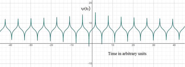
Figure 1.

Superimposed wave function ${\mathrm{\psi }}_{\mathrm{S}}\left({\mathrm{t}}_0\right)$ field distribution with time.

4. Results and discussions

An interesting fact is observed from the Figure 1 that the Standing wave pattern formed and has a Translational symmetry. This pattern is periodic and is repeated after a time interval “T”. This phenomenon is called “Distributed locality” which implies the same pattern is repeated throughout the space after regular time interval. Therefore once such pattern is formed, the information of spin is translated immediately between two entangled particles kept in far apart [2]. This forms a “String”. For an “N” dimensional observations there are “N” number of such strings which are superimposed to each other in different phases and amplitudes. Now, when we measure the spin at any end of the entangled pair particle at any particular direction or orientation, immediately the string correlated with the other directions or orientations collapses. This is called String lowering Operation.

When the measurement has taken place to calculate the Spin Orientation of an entangled particle for any particular direction; supposedly in the $\widehat{x}$ direction, we get:

$$\left|\psi \right.⟩=\frac{1}{\sqrt{2}}\left(\left|{\psi }_1\right.⟩+\left|{\psi }_2\right.⟩\right)$$E39

where, $\widehat{x}=\sqrt{\frac{\mathrm{\hslash }}{2\mathit{m\omega }}}\left(a+a^{†}\right)$

Now,

$$\begin{array}{lll}\left.⟨\psi \right|\widehat{x}\left|\psi \right.⟩& =& \frac{1}{2}\left.⟨\left(\left.⟨{\psi }_1\right|+\left.⟨{\psi }_2\right|\right)\right|\sqrt{\frac{\mathrm{\hslash }}{2\mathit{m\omega }}}\left(a+a^{†}\right)\left|\left(\left|{\psi }_1\right.⟩+\left|{\psi }_2\right.⟩\right)\right.⟩\\ & =& \frac{1}{2}\sqrt{\frac{\mathrm{\hslash }}{2\mathit{m\omega }}}\left.⟨\left(\left.⟨{\psi }_1\right|+\left.⟨{\psi }_2\right|\right)\right|\left|\left(\left|{\psi }_1\right.⟩+\left|{\psi }_2\right.⟩+\sqrt{2}\right)\left|{\psi }_3\right.⟩\right.⟩\\ & =& \frac{1}{2}\sqrt{\frac{\mathrm{\hslash }}{2\mathit{m\omega }}}\left(1+1\right)=\sqrt{\frac{\mathrm{\hslash }}{2\mathit{m\omega }}}\end{array}$$E40

We find a finite expectation value in the $\widehat{x}$ direction which is quiet obvious and all the others strings are immediately readjusted to “0” as follows:

We know, due to Ortho-normality conditions, $\left|\psi \right.⟩=\frac{1}{\sqrt{2}}\left(\left|{\psi }_1\right.⟩+i\left|{\psi }_2\right.⟩\right)=0$.

Therefore,

$$\begin{array}{lll}\left.⟨\psi \right|\widehat{x}\left|\psi \right.⟩& =& \frac{1}{2}\left.⟨\left(\left.⟨{\psi }_1\right|+i\left.⟨{\psi }_2\right|\right)\right|\sqrt{\frac{\mathrm{\hslash }}{2\mathit{m\omega }}}\left(a+a^{†}\right)\left|\left(\left|{\psi }_1\right.⟩+i\left|{\psi }_2\right.⟩\right)\right.⟩\\ & =& =\frac{1}{2}\sqrt{\frac{\mathrm{\hslash }}{2\mathit{m\omega }}}\left(1-1\right)=0\end{array}$$E41

This Operation is “String Lowering Operation”.

5. Conclusion

A particle with spin zero can be split into two particles whose spins are invariably opposite one another, giving rise to a sum of zero. Until the measurement is made, the quantum state of the spin does not “collapse” into either up or down; nevertheless, when the measurement is made, the other particle immediately assumes the opposing spin.

References

- 1.
Einstein A et al. Can quantum-mechanical description of physical reality be considered complete? Physical Review. 1935; 47 :777-780 - 2.
Chakrabarti K. Is there any spooky action at a distance? In: Maji AK, Saha G, Das S, Basu S, Tavares JMRS, editors. Proceedings of the International Conference on Computing and Communication Systems. Lecture Notes in Networks and Systems. Vol. 170. Singapore: Springer; 2021. DOI: 10.1007/978-981-33-4084-8_65 - 3.
Bennett C, Brassard G, Crepeau C, Jozsa R, Peres A, Wootters W. Teleporting an unknown quantum state via dual classical and Einstein-Podolsky-Rosen channels. Physical Review Letters. 1993; 70 :1895-1899 - 4.
Chakrabarti K. Realization of original quantum entanglement state from mixing of four entangled quantum states. In: Castillo O, Jana D, Giri D, Ahmed A, editors. Recent Advances in Intelligent Information Systems and Applied Mathematics: ICITAM 2019. Studies in Computational Intelligence. Vol. 863. Cham: Springer; 2020. DOI: 10.1007/978-3-030-34152-7_12 - 5.
Kharzeev DE. Quantum information approach to high energy interactions. Philosophical Transactions on Royal Society A. 2022; 380 :20210063. DOI: 10.1098/rsta.2021.0063