Wind Tunnel Measurement Techniques

Abstract

This chapter discusses different measurement techniques of a low-speed wind tunnel designed and built at the Faculty of Engineering and Built Environment, Universiti Kebangsaan Malaysia (UKM). The fully automated wind tunnel is named Pangkor after an island in Perak, Malaysia. Different measurement techniques are used to understand and validate the flow quality of the turbulent boundary-layer profiles at different locations and directions (wall-normal and spanwise). A hot-wire sensor captures the boundary layer over a smooth, flat surface. These data are then compared with high-quality published data. The flow uniformity shows comparable velocity variations and turbulent intensity. The boundary-layer profiles collapse well in different spanwise locations. Furthermore, the boundary-layer profiles at different ${\mathit{Re}}_{\tau }$ follow the standard boundary-layer profile. Since the wind tunnel is relatively new, the calibration method for the hot-wire anemometry is provided. The approach to spectral analysis is provided using a fast Fourier transform (FFT), revealing the prominence of the energized structure of ${{\lambda }_x}^{+}\approx 1000$ residing in the near-wall, in this analysis, we chose $z^{+}\approx 15$. The spectral analysis shows that the compounded effects of small and large-scale do not vary with ${\mathit{Re}}_{\tau }$. Nonetheless, the outer hump is increasingly visible with increasing ${\mathit{Re}}_{\tau }$. The proposed measurement technique and findings help validate wind tunnel flow quality and turbulent boundary layer profiles.

1. Introduction

Wind tunnels have been essential for aerodynamic research since the dawn of aviation [1]. Despite changes in their role and occasional predictions of their obsolescence, this situation is unlikely to change in the foreseeable future. Therefore, up-to-date measurement techniques are worthwhile. Constructing a new low-speed wind tunnel to study the fundamentals of turbulent boundary layers is a challenging endeavor that requires a profound comprehension of boundary layer dynamics and wind tunnel design [2]. These tunnels must undergo thorough testing to simulate typical boundary layer profiles with minimal turbulence intensity accurately. Extended wind tunnel studies are essential for advancing novel aircraft, wind turbines, and other systems that delicately interact with airflow. Low-speed aerodynamics is gaining popularity in both industry and academics. Despite the progress made in numerical models, low-speed wind tunnels remain essential in research and design procedures due to their unparalleled capacity to offer precise real-world data [3]. A smooth, turbulent boundary layer is necessary for sensitive experiments, where a high-quality flow becomes increasingly important [4]. One of the main variables affecting flow in a wind tunnel is the severity of turbulence. During the wind tunnel design process, much work is put into ensuring that the test section flow may have low levels of turbulence and stability. The main methods employed in the flow straightening and turbulence reduction system are contractions, honeycomb, and wire-mesh screens [5]. Most studies agreed that the screens and contractions reduce turbulence and mean velocity variation more in the longitudinal than in the lateral direction [3]. In the present research, a new low-speed wind tunnel was built in the Mechanical and Manufacturing Engineering Department, Universiti Kebangsaan Malaysia. This study aims to provide different measurement techniques using hot-wire anemometer. This method would help understand the turbulent boundary layer flow in wind tunnels.

2. Methodology

This study intends to systematically evaluate and validate the turbulent boundary layer profiles in a newly built wind tunnel. An extensive amount of data was gathered by employing various measuring approaches, each offering a unique set of benefits. A complete comparison and validation of the characteristics of the turbulent boundary layer were carried out by comparing the current data to high-quality published data [6, 7]. This was accomplished by employing sophisticated analytical tools to evaluate the data. A more reliable and in-depth understanding of turbulent boundary layers is vital for advancing wind tunnel and fluid mechanics.

2.1 Wind tunnel layout

Despite being owned by the Mechanical and Manufacturing Engineering Department, the Pangkor low-speed wind tunnel (PLSWT) is located at the Coastal and Water Resources Laboratory of the Faculty of Engineering and Built Environment, Universiti Kebangsaan Malaysia (UKM). The laboratory belongs to the Department of Civil Engineering, where research on waves, hydraulics using a wave maker, and channel flows are conducted. The wind tunnel has been developed and fine-tuned for the current research to improve flow quality and the turbulent boundary layer pattern. The wind tunnel is powered by a 15 kW AC axial fan, followed by a flexible duct, transition duct, diffuser, settling chamber, contraction nozzle with an area ratio of 2.4:1 and a test section with cross-sectional area 1.2 × 0.476 m (width × height) and 3 m total length. Figure 1 shows a general outline of the wind tunnel’s main parts. Figure 2 shows the actual photo of the wind tunnel.

Figure 1.

General outline of Pangkor low-speed wind tunnel.

Figure 2.

Pangkor low-speed wind tunnel. The left photo shows the main parts of the wind tunnel, starting from the transition duct to the contraction nozzle. The second photo shows the test section, and the traverse system is on the top of the ceiling.

The design and construction of the PLSWT started in 2014. The wind tunnel operated for the first time in September 2015 with a turbulence intensity level of 5%. To start with, the wind tunnel had only minimal measures to address turbulence intensities, that is, two meshing screens at the diffuser section. However, this value needed to be more suitable for the researchers to perform experiments to study the fundamentals of the turbulent boundary layer. In 2017, the second stage started with combining honeycomb and meshing screens to fine-tune the turbulent boundary layer profile and flow quality. Four new layers of meshing screens and a low-cost honeycomb built in-house, a three-dimensional plywood frame with dimensions of height, h = 1200 mm, width, w = 1200 mm, length, l = 200 mm, and thickness, t = 3 mm, were used as the main frame structure for the honeycomb. This frame is filled with 10,000 cells of circular plastic straw with diameter dimensions $d_s=12$ mm, length $l_s=177.5$ mm, and straw thickness $t_s=0.2$ mm. The honeycomb was installed in the middle of the setting chamber, where two layers of meshing screens were placed downstream of the honeycomb device. The last two layers are installed upstream to the honeycomb wall, to be six layers of the meshing screen in total [5]. For further information about the calculations of the meshing screen and honeycomb design, see Refs. [5, 8, 9]. The primary purpose of the honeycomb device and meshing screen in the wind tunnel is to support the flow homogeneity and the turbulence fluctuation and also to adjust the direction of the incoming flow to the test section. They resulted in a very low free-stream turbulence level of 0.0085% (see Figure 3).

Figure 3.

The variation of the mean velocity profile (a) and turbulence intensity (b) over the spanwise direction (y) of the wind tunnel. The vertical red dashed line indicates the center of the test section in a vertical direction.

In early 2018, serious development and fine-tuning for the wind tunnel were achieved. A new floor made of solid wood has been installed. Also, three stages of tripwires were used to develop the boundary layer. Therefore, this converted the wind tunnel to be the first for turbulent boundary layer studies in Malaysia with a minimum velocity variation and turbulence intensity value. For further information about the list of wind tunnels in Malaysia, see a review paper by Wiriadidjaja et al. [10].

2.2 Traverse construction

The traversing mechanism regulates the motion required for the installed sensors, such as the Pitot tube, hot-wire, or temperature probes, in both the vertical and horizontal directions. This enables various motions that may cover many locations within the examined sample. A two-dimensional (2D) traverse system designed and manufactured in-house includes two sliders firmly positioned within two sets of guides. These guides can be positioned vertically or horizontally and sit above the ceiling of the test section. Two fine-stepper motors facilitate the propulsion for this traverse. Therefore, each revolution necessitates 800 steps. The Vecta Steppers motors, specifically the PK266-034 model, are connected to Velmex controllers, the VXM-3 model. These motors are fitted with ball screws with a pitch of 1.6 mm, which applies to vertical and horizontal movements. The traverse provides a level of precision of less than 0.1 mm, or 4 × 10⁻³ mm for each step. This precision is necessary to capture the velocity fluctuations especially in the near-wall region. The motor controllers provide good support because communication can be established with many programming languages.

2.3 Data acquisition and automation

The most essential features of the wind tunnel are its functionalities and ease of use. A single-point control is preferred because operations can be made simple. Scilab is the only software for controlling air flow speeds, traverse systems, and acquisition operations. Starting from the motor, a National Instrument (NI) data acquisition (DAQ) system sends signals to the variable frequency drives (VFD). The fan speed was controlled through an output voltage signal produced by the NI DAQ 6008 module. This procedure is essential for hot-wire calibration. The atmospheric conditions, for example, atmospheric pressure (p), temperature (T), and relative humidity (RH), were measured using the Comet H7331 device for all experiments. The device was connected to the PC via a USB connection. The Modbus protocol was used to transfer data from the apparatus to Scilab. A simple Scilab code can then be elaborated to get the data from Comet H7331. A Velocicalc-TSI/9565A device was installed to get the mean flow velocity. The instantaneous velocity was measured using a Dantec hot-wire anemometer. A Dantec adapter conditioned the signal of the hot wire and then an NI DAQ 9215 module, which is connected to the Multichannel Constant Temperature Anemometers (CTA) and, therefore, via USB connected to the PC. Data were collected using an existing data acquisition box connected to a laptop using Scilab. The current data acquisition box can handle high requirements of at least a 100 kHz sampling rate with at least four channels in operations. A high-frequency rate is required to detect the energetic near-wall and large-scale features using the energy spectrum method [5, 11].

2.4 Calibration procedure

The hot-wire sensor is calibrated within the wind tunnel in all experimental series, employing a Pitot tube. The calibration process is conducted twice throughout each experiment, known as pre-calibration and post-calibration. To properly calibrate the hot-wire sensor, it is necessary to position it at a free-stream location, specifically at the center of the test section. Following that, it is essential to systematically measure and record a series of velocities, incrementally ranging from zero up to about 50% beyond the free-stream velocity deemed necessary for the experiment. Consequently, a polynomial third-order fitting is employed to establish a relationship between the voltage measured by the hot wire and the velocity measured by the Pitot tube. A comparison sample of calibration data is presented in Figure 4. This example includes both pre-calibration and post-calibration data. The pre-calibration and post-calibration curves are not expected to collapse because of expected temperature drift. A temperature drift of 1°C is usually acceptable.

Figure 4.

Hot-wire calibration curve for $U_{\infty }\approx \mathit{12}m/s$; where $\circ$ is pre-calibration and $\diamond$ is post. Poly. stands for polynomial fitting of the data.

Even though there is an increasing variation as velocity is increased as shown in Figure 4, the current comparison is deemed acceptable. When there is a large temperature drift that can be caused by the wind tunnel fan that keeps producing heat or simply because the building absorbs more energy as the sun rises, a temperature compensation procedure can be implemented. A temperature compensation is a procedure when an interpolation between pre- and post-calibration is performed. A typical acceptance criterion is the free-stream velocity should be within 2%.

2.5 Determining initial distance between wall and hot wire

A manual measurement established the distance between the hot-wire sensor and the wall. The distance was determined accurately by employing a high-resolution camera and a ruler. An exact traverse system was crucial for effectively controlling the exact movement of the hot wire in millimeter increments. Consequently, the hot-wire sensor was positioned successfully at approximately z = 0.25 mm from the wall. This distance directly influences the effectiveness of capturing the inner region of the turbulent boundary layer, particularly the inner peak. The positioning of the hot wire, including its inclination and yaw angle, followed the proposed method by Hutchins & Choi [12]. It is essential to use the strategy that has been provided in order to traverse the hot wire close to the wall before prong contact takes place. However, the traverse movement is no longer immediately connected to a wire movement after any wall contact has been made. The consequence at this point is that it leads to inaccurate measurements or hot-wire deformation (broken hot-wire sensor) (Figure 5).

Figure 5.

Determining the distance between the wall and hot wire using the physical method.

3. Results and discussion

3.1 Flow uniformity

In order to ensure that the wind tunnel has a high-quality flow condition, a spanwise measurement was performed to analyze the velocity and turbulence intensity variability profiles. The measurements were conducted at the center of the test section at a distance of wall-normal z = 250 mm and streamwise distance of x = 1.5 m with a free-stream velocity of $U_{\infty }=1.6\mathrm{m}/\mathrm{s}$. The velocity and turbulence intensity along the center line of the wind tunnel are shown in Figure 3. A hot-wire sensor was used to measure the velocity fluctuation at a frequency of 50 kHz for 180 seconds to ensure sufficient data capture. In the current measurements, the hot-wire platinum wire of 5 μm was used with a length of approximately 1.5 mm, and an overheat ratio was set between 1 and 1.5, similar to typical boundary layer studies [11, 13]. Unfortunately, the traverse movement is limited to only 400 mm in the spanwise direction ($y$), resulting in a total of 41 measurement points with a separation of 10 mm between each point. The velocity variation profile $\overline{U}/U_{\infty }$ plotted as a function of the spanwise direction ($y$) is shown in Figure 3(a), where the maximum deviation from the velocity profile ≈ 0.8%. The scaled turbulent intensity profiles ${\overline{u}}^2/U_{\infty }^2$ are shown in Figure 3(b). The profile indicates that the turbulent intensity variability is less than 10%, which is considered within acceptable limits. The mean value of the turbulent intensity in the wind tunnel ≈ 0.0085%. In summary, the wind tunnel exhibits good flow conditions to perform fundamental investigations on turbulent boundary layers and engineering applications, including airfoils, wind turbines, and surface roughness.

3.2 Turbulent boundary layer variability

A further check on the flow condition was performed. However, the focus this time is not on the homogeneity of flow in the center of the test section but on evaluating the quality of the turbulent boundary layer profile in various spanwise directions (y), as indicated in Figure 6. This is done to guarantee that the wind tunnel’s boundary layer profile follows the standard pattern and does not suffer from any defect. Figure 6 shows the wind tunnel test section and the location of spanwise measurements. The solid red line indicates the center of the test section, denoted by the letter C. The dashed red lines show the spanwise location of the turbulent boundary layer measurements denoted by 20 L, 10 L, 10R, and 20R. The letters L and R indicate the left and right directions about the center. The meaning of 10 L is that the measurement point shifted 100 mm to the left direction from the center point (C), and 20 L is shifted 200 mm from the center point (C). The points 10R and 20R shifted in the right direction from the center point (C). In the current experiment, there are five measurement points, each point separated by 100 mm, thus a coverage of 400 mm.

Figure 6.

Schematic diagram of the turbulent boundary layer measurements in different spanwise locations (y). The solid red line indicates the center of the test section, denoted by the letter C.

The wind tunnel is set to a free-stream velocity of $U_{\infty }\approx 5\mathrm{m}/\mathrm{s}$ subjected to favorable pressure gradient (FPG) environment. Measurements were made with a locally fabricated sensor soldered to a single hot-wire boundary layer type prob. with a core diameter of 5 microns (μm) [14]. All measurements were performed at the same streamwise distance $x/l=50\%$ in the test section length percentage, where $l$ is the test section length. In each boundary layer measurement, the hot-wire sensor traverses 50 logarithmically spaced wall-normal positions starting at approximately 0.250 up to 200 mm. All measurements were performed at a frequency of 20 kHz for 180 s, which represents boundary layer turnover times of ${\mathit{TU}}_1/d\approx 94000$ (T is time in seconds, $U_1$ is local free-stream velocity, and $\delta$ is the boundary layer thickness), which is more than sufficient for capturing the large-scale features in the near-wall region [7, 15, 16]. This section discusses and compares the statistical analysis of all five points over the smooth surface of the wind tunnel by analyzing the diagnostic plot, mean velocity, velocity defect, and turbulent intensity.

3.2.1 Diagnostic plot

The diagnostic plot was introduced by Alfredsson et al. [17] and Alfredsson et al. [18] as a method for evaluating the quality of the turbulent boundary layer. One significant feature of the diagnostic plot is that it does not require knowing the wall position or the friction velocity, therefore ensuring the elimination of any confusion relating to the position of the wall and the velocity related to friction. In their investigation of a smooth-wall turbulent boundary layer subjected to a zero pressure gradient (ZPG) environment [17, 18, 19, 20], it has demonstrated that the turbulent intensity, represented by $u_{\mathit{rms}}/U$, exhibits a linear decline with $U/U_{\infty }$ throughout the entire range spanning from the logarithmic to the wake region. Moreover, it can be shown that the linear zone expands as the friction Reynolds number ($\mathit{Re\tau }$) grows. In this region, all profiles exhibit a satisfactory collapse within the range of $0.5\le U/U_{\infty }\le 1$. Figure 7 shows the diagnostic plot over the smooth surface of the wind tunnel bed for five different locations in the spanwise direction. All profiles show a clear pattern and collapse very well for the entire region within the range of $0.6\le U/U_{\infty }\le 1$, which indicates that the turbulent boundary layer profiles in the current wind tunnel do not experience any defects and have high-quality data.

Figure 7.

Diagnostic plot of smooth turbulent boundary layer variability. Symbols ($⊲$) represent the point at 20 left, ($\Delta$) 10 left, ($\nabla$) 10 right, ($⊳$) 20 right, and the solid black line shows the measurements at the center of the test section.

3.2.2 Turbulence statistics: velocities and turbulence intensity profiles

Given the lack of direct measurements of ${\tau }_w$, the frictional velocity $U_{\tau }$ of the smooth wall needs to be estimated from the measured velocity profiles. The current study utilizes the Clauser method [21, 22] to determine the value of $U_{\tau }$. This is achieved by fitting the measured mean velocity to a log-law function with constants $\mathit{\text{kappa}}=0.41$ and an intercept A = 5.0 [23]:

$$U^{+}=\frac{1}{\kappa }ln\left(\frac{{\mathit{zU}}_{\tau }}{\nu }\right)+A,$$E1

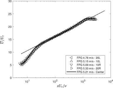
Figure 8 shows the mean velocities profile comparison between five locations in the spanwise direction. The velocity scaled with the skin-friction velocity $\mathit{U\tau }$ and the wall-normal length is made nondimensional by inner scaling of $\nu /U_{\tau }$, where $\nu$ is the kinematic viscosity. It shows a good agreement between all five profiles and collapses well in the near-wall region, logarithmic later, and the wake region.

Figure 8.

Comparison of the mean velocity profiles of turbulent boundary layer of five points in the spanwise direction (y). The dashed-dot black line indicates the log law, here κ = 0.41 and a = 5.0. Symbols ($⊲$) represent the point at 20 left, ($\Delta$) 10 left, ($\nabla$) 10 right, ($⊳$) 20 right and the solid black line shows the measurements at the center of the test section.

Figure 9 shows the velocity defect of all five profiles. The experiment data show an excellent agreement for the entire boundary layer. However, the current profiles do not follow the standard behavior of a turbulent boundary layer subjected to zero pressure gradient (ZPG). When the boundary layer is subjected to ZPG environment, the outer layer similarity profiles collapse well and agree with Townsend’s outer layer similarity [7, 24]. In other words, all the profiles in the ZPG case collapse well with the velocity defect low, represented by the following equation,

Figure 9.

Comparison of the velocity defect of five points in the spanwise direction. The dashed black line represents the defect low. Symbols ($⊲$) represent the point at 20 left, ($\Delta$) 10 left, ($\nabla$) 10 right, ($⊳$) 20 right, and the solid black line shows the measurements at the center of the test section.

$$\frac{U_{\infty }-U}{U_{\tau }}=-\frac{1}{\kappa }ln\left(\frac{z}{\delta }\right)+B$$E2

where $\kappa$ is the Karman constant, and B is the velocity defect constant; in the current study, B = 3. In the current study, all profiles collapse well. However, they shifted downward due to the effects of a favorable pressure gradient (FPG). The pressure gradient data provided by Harun [7] showed effects similar to those of the current experiment when the boundary layer was subjected to a favorable pressure gradient (FPG). The opposite effects can be seen when the boundary layer was exposed to an adverse pressure gradient (APG), where the velocity defect profile is shifted upward. The downward and upward shifts are due to the difference in skin friction velocity between the FPG and APG environments.

Figure 10 compares the turbulent intensity profiles of all five locations. The inner peak follows the standard boundary layer profile at z⁺ = 15, which has the highest level of turbulent intensity. There is an entirely different level of turbulent production in the near-wall region due to a lower free-stream velocity, particularly at the location 20 L, compared to other experiments. This results in a lower skin-friction Reynolds number ${\mathit{Re}}_{\tau }$, therefore, low frictional velocity, which affects the scaling of the profiles. However, the differences between the profiles on the near-wall region are acceptable. In the outer region, the profiles collapse very well. Most notably, the turbulent intensity at $z^{+}\ge 1000$ shows a very low turbulent intensity, close to zero. Figure 11 shows the turbulent intensities profiles wall-normal $z$ scaled with boundary layer thickness $\delta$. The boundary layer collapses very well in the outer region, which indicates the boundary layer thickness $\delta$ for all profiles is similar at similar $U_{\infty }$. In summary, the analysis of the variability of the turbulent boundary layer in the spanwise direction demonstrates a high level of agreement. The profiles show acceptable collapse behavior, and the flow quality is very high across the smooth surface.

Figure 10.

Comparison of the turbulent intensities of five points in the spanwise direction. Symbols ($⊲$) represent the point at 20 left, ($\Delta$) 10 left, ($\nabla$) 10 right, ($⊳$) 20 right, and the solid black line shows the measurements at the center of the test section. The black dashed-dot line indicates the location of inner peak at z⁺ = 15.

Figure 11.

Comparison of the turbulent intensities of five points in the spanwise direction. Symbols ($⊲$) represent the point at 20 left, ($\Delta$) 10 left, ($\nabla$) 10 right, ($⊳$) 20 right, and the solid black line shows the measurements at the center of the test section.

4. Flow validation and smooth-wall case

An experiment of a wall-normal was performed over the smooth wall at three different free-stream velocities $U_{\infty }=5$, 8 and 10 m/s at the exact free-stream location x = 1.5 m, and then compared to high-quality experimental data taken from Harun [7]. The taken data are subjected to FPG with different pressure gradient parameters β = −0.52, −0.43, −0.42, and − 0.33. This section analyzes and discusses the diagnostic plot, the inner- and outer-scale of the mean velocity profile and turbulent intensity, the velocity defect for both data and the spectral analysis of the current experiment. Table 1 shows the experimental parameters for the current study. The current section is divided into three main sections: diagnostic plot, turbulent statistic, and spectral analysis.

Exp Code	Surface Type	Location $x/l$%	$U_{\infty }$ (m/s)	$\delta$ (mm)	$U_{\tau }$ (m/s)	$\mathit{Re\tau }$
S	Smooth	50	5.22	87.3	0.2241	1204
S	Smooth	50	8.01	115.2	0.3380	2395
S	Smooth	50	10.27	127.8	0.4250	3410

Table 1.

Experimental parameters for smooth surfaces, $l^{+}={\mathit{lU}}_{\tau }/\nu \approx 15-30$ for all.

4.1 Diagnostic plot

Figure 12 compares the diagnostic plot of the smooth surface and the smooth pressure gradient data taken from Harun [7]. The top figure shows the classical scaling of the diagnostic plot, where the turbulent intensity $u_{\mathit{rms}}$ is scaled with $U$ as a function of $U/U_{\infty }$. In the top figure, the profile does not collapse well for the entire region due to pressure gradient effects. Recently, Drozdz et al. [25] have introduced a new scaling of the diagnostic plot for the turbulent boundary layer exposed to the pressure gradient effects, where the shape factor $H$ involved in the scaling of $u_{\mathit{rms}}/U$ to be $u_{\mathit{rms}}/\left(U\sqrt{H}\right)$. The new procedure provided a correct pattern for the diagnostic plot for pressure gradient flow, where all profiles collapse very well at $0.8\le \mathrm{U}/U\infty \le 0.9$. This is agreed well with the finding of Drozdz et al. [25].

Figure 12.

Comparison of diagnostic plot of the smooth data of the current experiments and FPG data taken from Harun [7], the data presented by the solid colored lines. The top plot shows the classical scaling, and the bottom plot shows the new scaling of diagnostic plot for the pressure gradient data.

4.2 Turbulence statistics: velocities and turbulence intensity profiles

Figure 13 shows the velocity and turbulent intensity profiles. The current comparison between all profiles of the current experiments is represented by the symbols ($\circ$), ($\diamond$), and ($\nabla$) and the colored solid lines represent the data taken from Harun [7]. The current plots are scaled with the skin-friction velocity $U_{\tau }$ as a function of scaled wall position $z^{+}={\mathit{zU}}_{\tau }/v$. The velocity profile shows that both data are collapsed very well in the inner region, logarithmic layer in the range of 100 ≤ z⁺ ≤ 0.15Re_τ. However, it is not the wake region, where the data have a different Reynolds number ${\mathit{Re}}_{\tau }$ and is performed in different facilities with different flow environments. The turbulent intensity profiles show the maximum turbulent production at z⁺ = 15, which follows the standard features of the turbulent boundary layer [6, 7]. However, the data that are taken from Harun [7] show a lower turbulent production, even though the data have a higher Reynolds number ${\mathit{Re}}_{\tau }$ as it is not supposed to be. When the Reynolds number increases, the near-wall peak also increases [6, 7, 15, 26]. However, the difference in both cases is due to the effect of different wind tunnel environments and spatial attenuation issue. In other words, the hot-wire sensor length $l^{+}$ [27].

Figure 13.

Comparison of mean velocity and turbulent intestines of the smooth data of the current experiments and FPG data taken from Harun [7], the taken data presented by the solid colored lines. The top plot shows the mean velocity profile, the black dashed-dot line represents the log-low. The bottom plot shows the turbulent intensity, where the black dashed-dot line shows the location on the inner peak at z⁺ = 15.

Furthermore, Figure 14 shows the mean velocity profile (top) and turbulent intensity profiles (bottom) are scaled with the outer parameter. Where the velocity and turbulent intensity are normalized with free-stream velocity $U_{\infty }$ and the wall-normal scaled with the boundary layer thickness $\delta$. The result of velocity profiles shows that all profiles collapse well at the wake region $z/\delta =0.8$. The turbulent intensity results collapse at $z/\delta =0.8$. This difference is due to different boundary layer thicknesses between both data and the flow test facility.

Figure 14.

Comparison of mean velocity and turbulent intestines of the smooth data of the current experiments and FPG data taken from Harun [7], the taken data presented by the solid colored lines. The top plot shows the mean velocity profile and the bottom plot shows the turbulent intensity, where the dashed-dot line represents the outer peak at $z/\delta =\mathit{0.5}$.

Figure 15 compares the velocity defect between both experimental data. All the profiles show an excellent collapse for the entire boundary layer regions. All the profiles shifted downward due to the effect of the pressure gradient on the turbulent boundary layer [24, 28]. Overall, all the analyses provided for validating the smooth-wall case over the wind tunnel floor reveal that the turbulent boundary layer has high-quality data and follows the standard features for the boundary layer. All the differences between the current experiments and the referenced data taken from Harun [7] are within the acceptable limit.

Figure 15.

Comparison of velocity defect profile of the smooth data of the current experiments and FPG data taken from Ref. [7], the taken data presented by the solid colored lines. The black dashed line represent the velocity defect low.

4.3 Spectral analysis

A spectral analysis was conducted to evaluate and understand the distribution and significance of various scale features in the turbulent boundary layer in both the near-wall and outer regions. One way to illustrate this is by analyzing all possible length scales that can exist at a particular location with respect to the wall. A pre-multiplied streamwise energy spectra provide a quick way to understand this, as the length scale can be non-dismensionalized with the boundary layer thickness ($\delta$). To start with, it is necessary to compute the pre-multiplied streamwise energy spectra $k_x{\varphi }_{\mathit{uu}}$, where the expression $k_x$ represents the streamwise wave number, while ${\varphi }_{\mathit{uu}}$ represents the spectral density of the streamwise velocity fluctuations. ${\varphi }_{\mathit{uu}}$ is obtained by a correlation of a velocity fluctuation to itself and this is easily computed in many software using a fast Fourier transform (FFT). Here, $k_x=2\mathit{\pi f}/U$, where $f$ is the frequency, and $U$ is the local streamwise mean velocity. The velocity spectra are pre-multiplied so that the area under the curve of $k_x{\varphi }_{\mathit{uu}}$ on the semi-logarithmic plot is ${\overline{u}}^2$.

The streamwise length scale is presented by ${\lambda }_x$, where ${\lambda }_x=2\pi /k_x$. Here, the data are normalized with the local friction velocity $U_{\tau }$, and the wavelength is normalized with $v/\mathit{U\tau }$ and boundary layer thickness $\delta$_, as shown in the bottom and top axis. Figure 16(a) shows the energy spectra at z⁺ = 15 in the near-wall and at $z=0.5\delta$ in the outer region. Figure 16(a) shows that the flow at different free-stream velocity $U_{\infty }=5$, 8 and 10 m/s, having an energized structure of ${{\lambda }_x}^{+}\approx 1000$. The vertical line in Figure 16(a) denotes ${{\lambda }_x}^{+}=1000$, it can be observed that the peak energy occurs at this location, and there is little variation to the energy distribution across the three velocities.

Figure 16.

Individual energy spectral at selected location. (a) z⁺ = 15 in the near-wall region, and (b) $z=0.5\delta$ in the outer region. $\circ$, $\diamond$, $⊲$ represents the smooth surface at 5, 8, and 10 m/s, respectively. Vertical line in (a) shows ${{\lambda }_x}^{+}=\mathit{1000}$.

On the other hand, Figure 16(b) shows that the highest energy of the flow structure at the outer region of $z=0.5\delta$ has a length scale of $1\le {\lambda }_x/\delta \le 3$. The current results indicate that the turbulent boundary layer at PLSWT has features similar to those of a standard turbulent flow in wind tunnels [7, 15, 26]. Further analysis of the spectra map provides an overview of the energy distribution over the entire boundary layer for all flow profiles. Figure 17(a)–(c) represent the spectra map of the entire boundary layer for all three profiles. The spectra maps give details of the most energetic region in the boundary layer represented by symbol (+), which shows the inner peak occurs at z⁺ = 15. The outer peak presented by the symbol (×) shows a different energy level for all profiles due to the effects of different Reynolds numbers ${\mathit{Re}}_{\tau }$. As the ${\mathit{Re}}_{\tau }$ increase, the chance of observing the outer peak in the outer region becomes higher as shown in Figure 17(c) compared to Figure 17(a) and (b), which is due to the effects of large-scale features. Harun [7] shows similar effects when the boundary layer is subjected to a different pressure gradient environment (ZPG, FPG, or APG) or different friction Reynolds number ${\mathit{Re}}_{\tau }$.

Figure 17.

Spectra maps for the flow over wind tunnel smooth surface (a) 5 m/s, (b) 8 m/s, and (c) 10 m/s. Symbols (+) and (×) represent the near-wall and outer hump locations.

5. Conclusions

Flow quality and turbulent boundary layer experiments have been performed at the Pangkor low-speed wind tunnel (PLSWT). The measurements were carried out using a hot-wire sensor over a flat surface. Different measurement techniques were used to understand and validate the flow in the wind tunnel’s test section. The flow uniformity measurement shows excellent results, where the wind tunnel experiences very low-level velocity and turbulent intensity variation due to the effects of the meshing screen and honeycomb device. The turbulence statistical analysis, including diagnostic test, boundary layer velocity profile, outer layer similarity, and turbulent intensity of different spanwise locations, shows a very excellent collapse between all five locations; this indicates that the boundary layer profiles across the spanwise direction do not differ and not suffer from any defect. The analysis of the turbulent boundary layer at the center of the test section at different ${\mathit{Re}}_{\tau }$ shows a good agreement between all three profiles with the compared data. The spectra individual and spectra map analysis shows in detail the turbulent flow features including the streamwise wavelength as well as the location of the most energized region in the boundary layer. The current measurement techniques are useful for researchers working on wind tunnel flow validation. Future measurements of spanwise variability at different streamwise locations and inclination angles are worthwhile.

Acknowledgments

We would like to express our gratitude for the financial support provided by Universiti Kebangsaan Malaysia’s Research University Grant GUP-2020-015.

References

1.Baals DD. Wind Tunnels of NASA. Vol. 440. Scientific and Technical Information Branch, National Aeronautics and Space …; 1981
2.de Almeida O, Carnevalli F, de Miranda O, Neto F, Saad FG. Low subsonic wind tunnel-design and construction. Journal of Aerospace Technology and Management. 2018;10
3.Britcher C, Landman D. Wind Tunnel Test Techniques: Design and Use at Low and High Speeds with Statistical Engineering Applications. Academic Press; 2023
4.Scheiman J, Brooks JD. Comparison of experimental and theoretical turbulence reduction from screens, honeycomb, and honeycomb-screen combinations. Journal of Aircraft. 1981;18(8):638-643
5.Harun Z, Wan AW, Ghopa SA, Izhar Ghazali M, Abbas AA, Rasani MR, et al. The development of a multi-purpose wind tunnel. Jurnal Teknologi. 2016;78:6-10
6.Harun Z, Monty JP, Mathis R, Marusic I. Pressure gradient effects on the large-scale structure of turbulent boundary layers. Journal of Fluid Mechanics. 2013;715:477-498
7.Harun Z. The structure of adverse and favourable pressure gradient turbulent boundary layers [PhD thesis]. 2012
8.Cattafesta L, Bahr C, Mathew J. Fundamentals of wind-tunnel design. In: Encyclopedia of Aerospace Engineering. Wiley Online Library; 2010. pp. 1-10
9.Mathew J, Bahr C, Carroll B, Sheplak M, Cattafesta L. Design, fabrication, and characterization of an anechoic wind tunnel facility. In: 11th AIAA/CEAS Aeroacoustics Conference. Monterey, California: AIAA Aerospace Research Central; 2005. p. 3052
10.Wiriadidjaja S, Hasim F, Mansor S, Asrar W, Rafie ASM, Abdullah EJ. Subsonic wind tunnels in Malaysia: A review. Applied Mechanics and Materials. 2012;225:566-571
11.Harun Z, Abbas AA, Mohammed Dheyaa R, Ghazali MI. Ordered roughness effects on NACA 0026 airfoil. IOP Conference Series: Materials Science and Engineering. 2016;152:012005
12.Hutchins N, Choi K-S. Accurate measurements of local skin friction coefficient using hot-wire anemometry. Progress in Aerospace Sciences. 2002;38(4-5):421-446
13.Monty JP, Harun Z, Marusic I. A parametric study of adverse pressure gradient turbulent boundary layers. International Journal of Heat and Fluid Flow. 2011;32(3):575-585
14.Harun Z, Abbas AA, Lotfy ER, Khashehchi M. Turbulent structure effects due to ordered surface roughness. Alexandria Engineering Journal. 2020;59(6):4301-4314
15.Hutchins N, Marusic I. Evidence of very long meandering features in the logarithmic region of turbulent boundary layers. Journal of Fluid Mechanics. 2007;579:1-28
16.Monty JP, Hutchins N, Ng HCH, Marusic I, Chong MS. A comparison of turbulent pipe, channel and boundary layer flows. Journal of Fluid Mechanics. 2009;632:431-442
17.Henrik Alfredsson P, Örlü R. The diagnostic plot—A litmus test for wall bounded turbulence data. European Journal of Mechanics-B/Fluids. 2010;29(6):403-406
18.Henrik Alfredsson P, Segalini A, Örlü R. A new scaling for the streamwise turbulence intensity in wall-bounded turbulent flows and what it tells us about the “outer” peak. Physics of Fluids. 2011;23(4). Article Number: 041702
19.Henrik Alfredsson P, Örlü R, Segalini A. A new formulation for the streamwise turbulence intensity distribution in wall-bounded turbulent flows. European Journal of Mechanics-B/Fluids. 2012;36:167-175
20.Henrik Alfredsson P, Segalini A, Örlü R. The diagnostic plot—A tutorial with a ten year perspective. In: iTi Conference on Turbulence. Springer; 2021. pp. 125-135
21.Clauser FH. Turbulent boundary layers in adverse pressure gradients. Journal of the Aeronautical Sciences. 1954;21(2):91-108
22.Clauser FH. The turbulent boundary layer. Advances in Applied Mechanics. 1956;4:1-51
23.Nagib HM, Chauhan KA. Variations of von Kármán coefficient in canonical flows. Physics of Fluids. 2008;20(10). Article Number: 101518
24.Townsend AAR. The Structure of Turbulent Shear Flow. Cambridge University Press; 1976
25.Dróżdż A, Elsner W, Drobniak S. Scaling of streamwise Reynolds stress for turbulent boundary layers with pressure gradient. European Journal of Mechanics-B/Fluids. 2015;49:137-145
26.Hutchins N, Marusic I. Large-scale influences in near-wall turbulence. Philosophical Transactions of the Royal Society A: Mathematical, Physical and Engineering Sciences. 2007;365(1852):647-664
27.Harun Z, Isa MD, Rasani MR, Abdullah S. The effects of spatial resolution in turbulent boundary layers with pressure gradients. Applied Mechanics and Materials. 2012;225:109-117
28.Townsend AA. The Structure of Turbulent Shear Flow. Cambridge: Cambridge University Press; 1956
Written By
Zambri Harun and Ashraf Amer Abbas
Submitted: 29 January 2024Reviewed: 02 April 2024Published: 03 May 2024